Article

AI-Driven Digital Twin for Optimizing Solar Submersible Pumping Systems

1
Research and Innovation Center, Arab Academy for Science, Technology and Maritime Transport, Alamein 51718, Egypt
2
Artificial Intelligence Research Center (AIRC), College of Engineering and Information Technology, Ajman University, Ajman P.O. Box 346, United Arab Emirates
3
School of Mathematics and Computer Science, Herriot Watt University, Dubai P.O. Box 501745, United Arab Emirates
4
Department of Electrical Power Engineering, Faculty of Engineering, Damanhour University, Damanhour 22511, Egypt
*
Author to whom correspondence should be addressed.
Inventions 2025, 10(6), 93; https://doi.org/10.3390/inventions10060093
Submission received: 31 August 2025 / Revised: 19 October 2025 / Accepted: 22 October 2025 / Published: 25 October 2025

Abstract

Reliable water access in remote and desert-like regions remains a challenge, particularly in areas with limited infrastructure. Solar-powered submersible pumps offer a promising solution; however, optimizing their performance under variable environmental conditions remains a challenging task. This research presents an Artificial Intelligence (AI)-driven digital twin framework for modeling and optimizing the performance of a solar-powered submersible pump system. The proposed system has three core components: (1) an AI model for predicting the inverter motor’s output frequency based on the current generated by the solar panels, (2) a predictive model for estimating the pump’s generated power based on the inverter motor’s output, and (3) a mathematical formulation for determining the volume of water lifted based on the system’s operational parameters. Moreover, a dataset comprising 6 months of environmental and system performance data was collected and utilized to train and evaluate multiple predictive models. Unlike previous works, this research integrates real-world data with a multi-phase AI modeling pipeline for real-time water output estimation. Performance assessments indicate that the Random Forest (RF) model outperformed alternative approaches, achieving the lowest error rates with a Mean Absolute Error (MAE) of 1.00 Hz for output frequency prediction and 1.39 kW for pump output power prediction. The framework successfully estimated annual water delivery of 166,132.77 m3, with peak monthly output of 18,276.96 m3 in July and minimum of 9784.20 m3 in January demonstrating practical applicability for agricultural water management planning in arid regions.

1. Introduction

Access to reliable water resources is a fundamental challenge in many remote and arid regions. With climate change and water scarcity becoming crucial global concerns, solar-powered submersible pump systems have emerged as a sustainable and cost-effective solution [1,2,3,4,5,6,7,8]. By harnessing solar energy, these systems provide an environmentally friendly alternative to traditional water pumps, reducing dependence on fossil fuels and grid electricity. However, their efficiency is directly influenced by changing environmental conditions, such as solar radiation, temperature, wind speed, and humidity, which can affect power generation and overall performance [9,10,11,12,13,14,15,16].
Artificial Intelligence (AI) has demonstrated remarkable capabilities in addressing modern challenges, enabling optimization [17,18], event detection [19,20,21,22], and enhancement [23,24,25] across different domains. Moreover, Al has empowered the use of Digital Twins (DT) [26]. In order to achieve an optimized and predictive model for submersible pump systems, this research proposes an Al-driven digital twin by implementing machine learning models, and using the environmental conditions as input data to the system. The main aim is to ensure that the water volume pumped remains available even under fluctuating environmental conditions.
While digital twin applications in renewable energy have gained traction in recent years, most existing frameworks focus on performance monitoring or predictive maintenance of photovoltaic (PV) systems, ref. [27,28,29] without integrating multi-phase AI modeling for water output estimation. Similarly, prior AI-driven solar water pumping studies have explored adaptive control strategies [30] or hybrid MPPT algorithms, ref. [31] but these approaches typically optimize electrical parameters without modeling the full series from environmental inputs to hydraulic output. In contrast, our framework introduces a novel three-phase architecture that sequentially predicts inverter motor frequency, pump output power, and water volume using real-world data. Moreover, unlike digital twin models for submersible pumps that focus on thermal simulations or fault detection [32], our system integrates sensorless water volume estimation via hydraulic modeling, enabling cost-effective deployment in remote agricultural settings. These distinctions underscope the originality and practical relevance of our contribution to the field.
This study introduces a practical and intelligent framework that bridges renewable energy systems with advanced predictive analytics. Unlike traditional approaches that rely on static models or manual tuning, our work leverages real-world data and machine learning to create a dynamic digital twin for solar-powered submersible pumping systems. The key contributions are as follows:
  • We design an AI-driven architecture capable of predicting inverter motor frequency and pump output power under fluctuating environmental conditions, ensuring reliable water delivery in remote areas.
  • We integrate predictive intelligence with physical hydraulic modeling, enabling accurate estimation of water volume without additional sensors, reducing cost and complexity.
  • Through extensive experimentation on real operational data, we demonstrate that the Random Forest model consistently outperforms other techniques, achieving high accuracy with minimal computational overhead, making the solution suitable for real-time and edge deployments.
This combination of renewable energy, AI-based modeling, and digital twin technology positions our work as a step toward smarter, more sustainable water management solutions in resource-constrained environments.
The paper is structured as follows: Section 2.1 provides a detailed overview of the system design. Section 2.2 describes the dataset used for training and evaluation. The proposed methodology is outlined in Section 2.3, followed by the presentation and analysis of results in Section 3. Finally, the conclusions and future research directions are discussed in Section 5.

2. Materials and Methods

This section describes the system design, dataset collection, methodology for model development, and experimental setup used in this study.

2.1. System Design

The system is designed to lift water from a water well reservoir in a remote desert-like area. The system is designed to fully operate on solar energy. Figure 1 shows a schematic illustration of the system. The system consists of:
  • Solar panel: Suntech STP340-A72/Vfh, model specifications are shown in Table 1.
  • Inverter motor: YASKAWA AC Drive GA700, model specifications are shown in Table 2.
  • Pump: Vansan VSPss04090/6.B2, model specifications are shown in Table 3.
  • Motor (powering the pump): Vansan VSMOF4/30T, model specifications are shown in Table 4.

2.2. Dataset

Data were collected for a 6-month period in order to train and evaluate predictive AI models. The system described in Section 2.1 was operated, and data were collected in the Khataba region in Elsadat, Beheira Government in Egypt. 110,022 records were collected. The dataset collected consisted of two categories: weather data and inverter motor data.
The weather data comprises:
  • UV index measured by (W/m2)
  • Air temperature measured by degree Celsius (°C)
  • Wind speed measured by (m/s)
  • Wind direction measured by degrees from North
  • Humidity measured by percentage
  • Gust measured by (m/s)
  • Cloud cover measured by percentage.
The energy generated by solar power is influenced by various environmental factors. For example, a higher UV index generally increases energy output since solar panels rely on sunlight, though prolonged exposure can degrade materials over time [33,34]. Air temperature, on the other hand, has a negative impact on the energy generated. However, while solar panels need sunlight, excessive heat reduces efficiency due to increased electrical resistance, therefore, wind speed can be beneficial in cooling the panels, helping to counteract temperature-related losses, but strong gusts may stress mounting structures. Wind direction indirectly affects performance by influencing cooling efficiency, depending on how air flows around the panels [35,36]. On the other hand, humidity reduces energy output because water vapor scatters sunlight, limiting the amount of radiation reaching the panels, and over time, excessive moisture can degrade panel components. Similarly, cloud cover reduces the effect of direct sunlight, leading to lower energy production [37]. Overall, optimal conditions for solar energy include high UV levels, moderate temperatures, steady cooling winds, and minimal humidity or cloud cover. The weather data were collected daily using the stormglass.io API, given a certain position in terms of longitude and latitude. This data represents the parameters that affect the solar energy, hence the input power to the inverter motor. On the other hand, the data related to the inverter motors are:
  • Frequency reference
  • Output frequency
  • Output current
  • DC bus voltage
  • Output power
  • Output frequency fault
  • Heatsink temperature
  • Proportional-Integral-Derivative (PID) controller output
  • PID input
Inverter motors work by controlling a range of input and output parameters to keep the motor running. One of the main inputs is the frequency reference, which sets the target speed by controlling the AC frequency sent to the motor. Moreover, a PID input adjusts the inverter’s PID controller to maintain optimal performance. On the other hand, the outputs include frequency, current, DC bus voltage, and power. The output frequency value is directly sent to the motor, affecting its speed. The output current represents the amount of electrical load being used, and the DC bus voltage is crucial for the inverter’s internal power consumption, ensuring a consistent power supply. Additionally, the output power indicates how much energy is delivered to the motor. Additionally, output frequency fault warnings are produced when the motor is not operating as expected. Lastly, the PID output value represents the system’s corrective action to adjust the motor’s output, then serves as an input to a connected pump motor. More details about the dataset is presented in [38].

2.3. Proposed Methodology

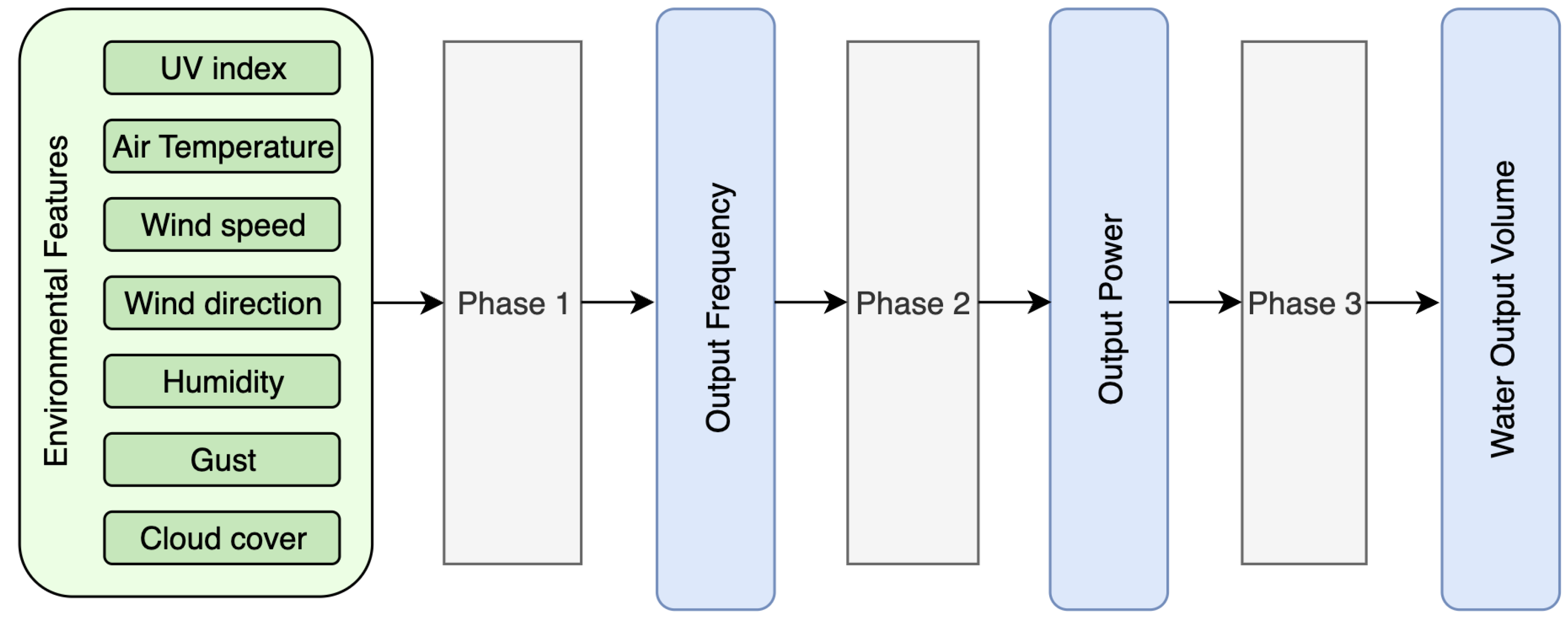
This section outlines the methodology used to analyze data and develop AI-based models that predict the performance of a solar-powered water pumping system. The first objective is to predict the output frequency of the inverter motor based on environmental conditions; the second objective is to utilize the predicted frequency to estimate the output power of the system. Finally, the third objective is to use the estimated pump output power to calculate the water output volume.
The complete process flow of the proposed AI-based predictive system is illustrated in Figure 2, which shows the three-phase architecture from data preprocessing through frequency prediction (Phase 1), power estimation (Phase 2), and water volume calculation (Phase 3).
Due to the fact that environmental conditions strongly affect system performance, different machine learning models are employed to explore data patterns and features. Data preprocessing is performed to remove noise and ensure consistent input to machine learning models. Moreover, different machine learning models are implemented to predict the output frequency based on weather conditions. Moreover, using this predicted frequency, the output power is then estimated. Finally, each machine learning model is evaluated using standard evaluation metrics.

2.3.1. Phase 1: Output Frequency Prediction

In this phase, the environmental factors, including UV index, air temperature, wind speed, humidity, and Frequency reference, are used as input to different predictive models in order to estimate the output frequency of the inverter motor.
Data Pre-Processing (Phase 1)
Data preprocessing is a crucial step before utilizing the environmental raw data inputs in predictive machine learning models. These raw data include noise, missing values, and inconsistent formats. Data preprocessing is crucial to help the models efficiently extract important features and achieve accurate predictions.
Handling Missing Values: The dataset used for this study was complete and had no missing values in any of its features. In addition to removing the need for imputation and reducing potential biases frequently associated with handling missing data, this guarantees the integrity and completeness of the input data for all prediction models [39,40].
Data Shuffling: To prevent any bias arising from the order of data points and to ensure that the models are trained on a diverse set of examples in each iteration, the dataset was reordered randomly.
Scaling Features: A targeted feature scaling strategy was used to maximize model performance and guarantee steady convergence, especially for algorithms like neural networks that are sensitive to the scale and range of input features. Because it effectively preserves the structure of the original data distribution while translating values to a precise, defined interval, Min-Max scaling—which uses Equation (1) to normalize feature values to a range between 0 and 1—was explicitly selected. Features with distinct physical boundaries or intrinsic percentage-based units benefit most from this approach [41,42].
‘Humidity (%)’ and ‘Frequency Reference’ were found to be the main contenders for Min-Max scaling in Phase 1. Normalization to 0–1 is understandable and advantageous for consistent model input because “Humidity (%)” naturally functions within a 0–100% range, with a maximum observed value of 85.02%. The ‘Frequency Reference’ is a critical control signal in a clearly defined operating band, with a maximum observed value of 50.00 Hz. In addition to facilitating more stable gradient propagation during Neural Network training, scaling these features to the [ 0 , 1 ] range guarantees that they contribute proportionately to the model’s learning process.
For these particular features, min-max scaling was chosen over standardization (Z-score normalization) for a number of reasons. According to Goodfellow (2016) [42], Z-score normalization converts data to a mean of zero and unit variance, but its unbounded output may not always be optimal for neural networks that use activation functions that demand inputs within a restricted range, such as [ 0 , 1 ] or [ 1 , 1 ] . Min-Max scaling provides a more straightforward and understandable mapping to a proportional 0–1 scale for features with intrinsic physical bounds, such as humidity and operational frequencies. This avoids potential distortions that could result from Z-score transformation on non-normally distributed or bounded data and is in line with the features’ physical meaning.
Other environmental features, namely ‘UV Index’ (maximum observed value of 0.27 W/m2), ‘Air Temperature’ (maximum observed value of 43.03 °C), and ‘Wind Speed’ (maximum observed value of 10.19 m/s), possess different measurement units and do not have the same strict upper bounds or percentage-based interpretations. These features were retained in their original scale as their raw magnitudes were deemed appropriate inputs for the chosen machine learning algorithms. Tree-based models like Random Forest and Gradient Boosting, which were primary performers in our study, are inherently robust to the scale of input features as they make decisions based on splits at feature values rather than distances [43]. For Linear Regression, while scaling can aid in convergence, the primary concern for gradient-sensitive models like Neural Networks was addressed through the selective Min-Max approach.
X = X X m i n X m a x X m i n
Data Partitioning: The carefully preprocessed dataset, consisting of 110,022 records, was subjected to a rigorous partitioning procedure to provide a robust and objective assessment of the predictive models. To ensure the randomness of sample distribution across all subsets and to minimize potential biases due to the temporal or sequential structure of data collection, the entire dataset was thoroughly shuffled before splitting. Subsequently, the randomized dataset was divided into three distinct subsets using an 80/10/10 split ratio. The training set, comprising 80% of the data, was used to fit the parameters of all predictive models, enabling the learning of robust patterns and relationships from the data. The validation set, representing 10% of the data, was used exclusively during the model development phase for model selection and hyperparameter tuning. It helped guide optimization and prevent overfitting, while preserving the integrity of the final model evaluation. The remaining 10% was assigned to the test set, which remained completely isolated throughout the training and validation phases and was used only once—after final model selection—to provide an unbiased estimate of the models’ generalization performance on new, unseen data. This 80/10/10 split strategy is consistent with recommendations in the literature for large-scale datasets, ensuring that sufficient data is available for training while still allocating an adequate portion (typically 10–30%) for validation and testing to support reliable model evaluation [42,44,45].
Machine Learning Models
The pre-processed data, utilizing UV Index ( W / m 2 ), Air Temperature (°C elsius), Wind Speed (m/s), Humidity (%), and Frequency Reference as input features, and Output Frequency as the target variable, was used to train and evaluate five machine learning models. The selection of these models was specifically designed to cover a spectrum of modeling approaches—from simple linear baselines [43,46] to complex non-linear ensemble methods [47,48,49] and deep learning architectures [42]—to comprehensively assess the structure of the feature-target relationship:
  • Random Forest: A Random Forest Regressor was implemented, an ensemble learning method that constructs multiple decision trees during training and outputs the average prediction of the individual trees. This model was chosen for its ability to model complex relationships between the environmental features and the output frequency without assuming linearity [47].
  • Linear Regression: A Linear Regression model was implemented to find the linear relationship between the environmental input features and the output frequency by minimizing the sum of squared errors [43,50]. This model was included as a baseline to assess the linearity of the relationship between the environmental factors and the frequency output [46].
  • Neural Network (NN1): A sequential Neural Network 1 (NN1) was constructed. The network consists of an input layer accepting 5 features (UV Index, Air Temperature, Wind Speed, Humidity, Frequency Reference), connected to hidden layers that use the ReLU activation function ( ReLU ( x ) = max ( 0 , x ) ) [51]. The output layer has a single neuron with no activation, predicting the continuous output frequency. The model was trained using the Adam optimizer, an algorithm that adapts the learning rate during training [52], with Mean Squared Error (MSE) as the loss function. Mean Absolute Error (MAE) was tracked as an additional metric. This architecture was chosen to capture potential complex, non-linear interactions between the environmental inputs and the resulting frequency.
  • Gradient Boosting: A Gradient Boosting Regressor was implemented by sequentially adding decision trees to correct the errors of previous trees. This model was selected for its potential to achieve high predictive accuracy by learning from the residuals of previous models in the ensemble [49,53].
  • XGBoost: Additionally, a XGBoost Regressor, a very effective and optimized gradient boosting solution. Because of its exceptional performance and regularization capabilities, which make it resistant to overfitting while retaining a high predictive power, XGBoost was selected [48].
Hyperparameter Tuning
Optimizing hyperparameters is essential for enhancing the performance of machine learning models and avoiding overfitting, especially when evaluating various model architectures. To facilitate a rigorous and equitable comparison between Linear Regression, Random Forest, Gradient Boosting, XGBoost, and a single Neural Network (NN1), a structured hyperparameter optimization approach, was executed for each model. All tuning efforts sought to minimize the Root Mean Squared Error (RMSE) on the specified validation sets or through cross-validation folds, aiming to identify the configurations that generalize most effectively to new data.
In the case of the Linear Regression model, the main hyperparameters are associated with regularization (such as 1 or 2 penalties for Lasso or Ridge regression, respectively). Due to its simpler structure and fewer tunable parameters, a Grid Search strategy was applied. This method systematically examined a predetermined range of regularization strengths α { 0.001 , 0.01 , 0.1 , 1 , 10 } , directly assessing each combination to find the optimal α that minimized RMSE on the validation set. The optimal regularization strength ( α ) found for the Ridge model was 0.1.
For the ensemble tree-based models, Random Forest, Gradient Boosting, and XGBoost, which have a larger set of interrelated hyperparameters, a Random Search with K-Fold Cross-Validation method was utilized. This strategy is considerably more computationally efficient than a comprehensive Grid Search in complex hyperparameter spaces while still effectively probing the search area. Specifically, 5-fold cross-validation was implemented on the training set for each sampled hyperparameter combination, with the average RMSE across the folds serving as the objective for optimization. The key hyperparameters and the corresponding search distributions for Random Forest included: (1) Number of Estimators corresponding to the number of trees in the forest, drawn from a uniform integer distribution between 100 and 1000, (2) Maximum depth of each tree, sampled from a uniform integer distribution between 5 and 20, or set to None to allow full growth, (3) Minimum Samples Split to split an internal node, sampled uniformly between 2 and 20, and (4) Minimum Samples Leaf corresponding to the minimum number of samples required at a leaf node, sampled uniformly between 1 and 10.
While the key hyperparameters for the Gradient Boosting included: (1) Number of Estimators corresponding to the number of boosting stages, sampled uniformly between 100 and 1000, (2) Learning Rate corresponding to the step size shrinkage applied in updates, drawn from a log-uniform distribution between 0.01 and 0.2, (3) Maximum Depth of the individual base estimators, sampled uniformly between 3 and 10, (4) Subsample Ratio, which is the fraction of training samples used for fitting each base learner, drawn from a uniform distribution between 0.6 and 1.0, (5) Maximum Features considered when determining the best split, sampled uniformly between 0.5 and 1.0, (6) Minimum Samples Split required to split an internal node, drawn uniformly between 2 and 20, and (7) Minimum Samples required at a leaf node, drawn uniformly between 1 and 10.
Also, the key hyperparameters for XGBoost included: (1) Number of Estimators corresponding to the number of boosting iterations, sampled uniformly between 100 and 1000, (2) Learning Rate, as a shrinkage factor for model updates to prevent overfitting, drawn from a log-uniform distribution between 0.01 and 0.3, (3) Maximum Depth of each tree, sampled uniformly between 3 and 10, (4) Subsample Ratio of training instances used per boosting round, sampled uniformly between 0.6 and 1.0, (5) Column Subsample Ratio by Tree corresponding to the fraction of features randomly selected per tree, drawn from a uniform distribution between 0.6 and 1.0, and (6) Gamma, which is the minimum loss reduction required to make a split, sampled from a log-uniform distribution between 0 and 0.5.
A total of 75 random hyperparameter combinations were evaluated for each model using cross-validation. The configuration with the lowest average Root Mean Squared Error (RMSE) across the validation folds was chosen as the final optimized set. The hyperparameters resulting for each model are shown in Table 5.
Neural Network 1 (NN1): For the Neural Network 1 (NN1) model, which is notably sensitive to initial conditions and architectural design, Bayesian Optimization was employed as the core tuning method. This probabilistic approach constructs a surrogate model of the validation RMSE objective function and leverages it to strategically select the most promising hyperparameter configurations, thereby minimizing the number of costly training evaluations. The optimization process was carried out on a separate validation set to effectively guide the search process.
Key hyperparameters considered in the tuning process included the learning rate applied to the Adam optimizer, sampled from a log-uniform distribution between 10 4 and 10 2 , and the batch size, selected from discrete values such as 32, 64, 128, or 256. The number of epochs, which represents complete passes over the training dataset, was typically allowed to range from 50 to 200 and was coupled with an early stopping mechanism to avoid overfitting. The depth of the network was controlled through the number of hidden layers (ranging between 1 and 3), and the model’s representational capacity was further adjusted by varying the number of neurons per layer, sampled uniformly from 16 to 128. To reduce overfitting, a dropout rate between 0.1 and 0.5 was also tuned.
Selection of Activation Function for NN1: The Rectified Linear Unit (ReLU) activation function was initially considered due to its computational efficiency and robustness against the vanishing gradient problem. However, alternative activation functions such as the Exponential Linear Unit (ELU) and Leaky ReLU were also included in the Bayesian Optimization search space. The final activation function was selected based on validation performance, ensuring that the most generalizable function was adopted for the final model.
Early Stopping and Training Epochs for NN1: The number of training epochs for NN1 was not fixed a priori. Instead, the training incorporated an Early Stopping mechanism that monitored the validation RMSE. If no improvement was observed for a defined number of consecutive epochs (a ‘patience’ parameter), the training was halted automatically to prevent overfitting. This allowed the training duration to adapt based on model performance rather than arbitrary constraints.
The final neural network configuration was the result of this thorough Bayesian Optimization process and represents a balance between predictive performance and training efficiency. The selected hyperparameters are summarized in Table 6.
Through a systematic approach to tuning each model’s hyperparameters using dedicated validation data or cross-validation, we ensured a robust and equitable comparison of all models’ predictive capabilities on the unseen test set.

2.3.2. Phase 2: Output Power Prediction

In this phase, the output predicted by the models in Phase 1 (Output Frequency) serves as the primary input feature to predict the final target variable: Output Power. Before applying the machine learning models, the data undergoes pre-processing.
Data Pre-Processing (Phase 2)
Data Shuffling: The dataset was randomly shuffled before model training in order to minimize any potential bias that could arise from the sequential structure of the predicted Output Frequency values. This method fosters solid generalization by stopping the model from becoming too tailored to localized patterns or temporal correlations in the data [42,44].
Data Partitioning: In keeping with the strict methodology developed in Phase 1, the preprocessed dataset for Phase 2 underwent the same meticulous partitioning process. Using the same 80/10/10 ratio, the dataset was systematically separated into three distinct subsets. The training set, comprising 80% of the data, was dedicated to fitting the parameters of all predictive models, enabling them to learn intricate patterns and relationships. The validation set, representing 10% of the data, was used exclusively during the model development phase for model selection and hyperparameter tuning. Its primary role was to guide optimization and reduce the risk of overfitting, thereby preserving the integrity of the final model evaluation. The remaining 10% constituted the test set, which remained entirely isolated throughout the training and validation processes. This subset was only used after final model selection to provide an unbiased estimate of the models’ generalization performance on unseen data. This continuous 80/10/10 split technique ensures sufficient data for training while maintaining enough reserved samples for reliable validation and testing, consistent with best practices for large-scale datasets.
Machine Learning Models
The modeling approach changes for Phase 2 in order to capitalize on the predictive strength of our earlier work. In contrast to Phase 1, the sole input feature for every model in Phase 2 will be the predicted output from the Random Forest Regressor [47], which was the best-performing model in Phase 1. By using the Random Forest’s output as a highly distilled and informative feature for additional refining or analysis, this method seeks to expand upon the first learnt correlations.
Each model will be used with this single, derived input in the following manner:
  • Random Forest: The output of the Phase 1 Random Forest will be used as the single input feature for training a new Random Forest Regressor. More intricate patterns within the original predictions themselves [47] may be captured in this way.
  • Linear Regression: When predicting the final target variable, a Linear Regression model will be used to evaluate any linear trends seen in the output of the Phase 1 Random Forest.
  • Neural Network (NN2): In order to learn non-linear modifications of these predictions, our sequential Neural Network (NN2) will be set up to accept a single input neuron (which corresponds to the output of the Phase 1 Random Forest) into its input layer. Activation functions like ReLU ( ReLU ( x ) = max ( 0 , x ) ) would probably be used by this network. and be optimized using methods such as Adam [52].
  • Gradient Boosting: The goal of a Gradient Boosting Regressor is to increase the predictive accuracy of this refined signal [53] by building decision trees in a sequential manner using only the one input feature obtained from the Phase 1 Random Forest.
  • XGBoost: Additionally, only the output from the Phase 1 Random Forest will be used as input for the XGBoost Regressor, an efficient gradient boosting solution. To get the most predictive power out of this pre-processed signal [48], its strong capabilities will be used.
Hyperparameter Tuning
Consistent with the methodology established in Phase 1, a comprehensive hyperparameter optimization process was rigorously applied to all machine learning models in Phase 2. The primary objective remained the minimization of the Root Mean Squared Error (RMSE) on validation sets or through cross-validation folds, ensuring the models generalize effectively to unseen data. The same structured search strategies were employed: Grid Search for Linear Regression, Random Search with K-Fold Cross-Validation for the ensemble tree-based models (Random Forest, Gradient Boosting, and XGBoost), and Bayesian Optimization for the Neural Network (NN2). For the Ridge Regression model, the optimal value for the regularization strength ( α ) was found to be 0.1. The final optimized hyperparameters for the tree-based models and the neural network are presented in Table 7 and Table 8, respectively. This structured tuning approach, tailored to each model’s architecture and training behavior, ensured fair and robust comparisons across all models evaluated in Phase 2.

2.3.3. Phase 3: Water Volume Prediction

This phase is the last phase in the proposed digital twin. In this phase, the output from phase 2 (the pump output power) is used to calculate the water output volume. In this research [54], Elrefai et al. presented a detailed methodology in order to calculate the water volume pumped from a submersible water reservoir based on a pump output power.
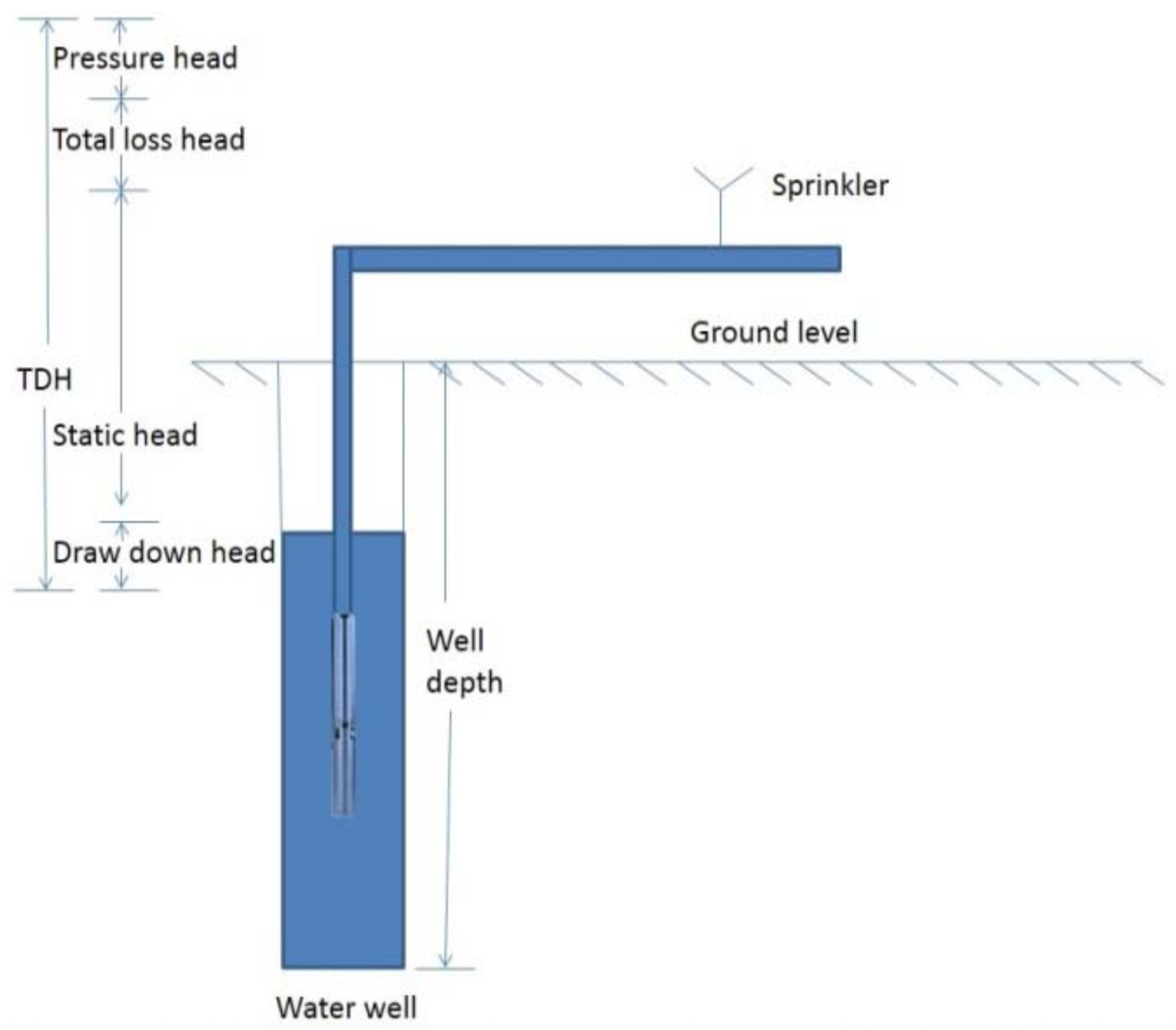
In order to calculate the water volume, a few calculations needs to be computed. First, the Total Dynamic Head (TDH), see Figure 3 for more details, which is the total equivalent height that a fluid is to be pumped, taking into consideration many energy losses and gains. It’s essentially the sum of all the components the pump has to overcome in order to move fluid through a system. The total dynamic head TDH could be expressed in Equation (2)
TDH = H s t + H d + H l + H p
According to Equation (2), the first parameter is the static head H s t measured in meters. According to the measures of the Khataba water reservoir, the H s t = 54 m, then the drawdown head H d measured in meters, the measurement shows that the H d = 1.5 m. the total loss head H l also measured in meters, H l = 11.7 m. Finally, pressure head H p = 20 m. Giving all these measure, the T D H = 87.2 m. The required hydraulic power P h (W) could be expressed as in Equation (3)
P h = ρ · g · TDH · Q 3600
In Equation (4), Q is the flow rate ( m 3 /s), ρ is the water density ( kg / m 3 ) , and g is the gravitational acceleration ( m / s 2 ) . The required pump capacity is determined by dividing the hydraulic power over the selected pump efficiency given as in Equation (4)
P 2 = P h η pump
Equation (4), computes the required pump input power P 2 . This can be computed giving the required hydraulic power P h over the pump efficiency η pump . Using the previous equations and information together, we form the equation for our System (5), to calculate Q in ( m 3 / h ) :
Q = P 2 · η pump ρ · g · TDH
Substituting the TDH, ρ and g we get Equations (6) and (7):
Q = P 2 · η pump 1000 · 9.81 · 87.2
Q = P 2 · η pump 855432
Giving that the pump efficiency used in the system 65%, we reach the final Equations (8) and (9):
Q = P 2 · 0.65 855432
Q = P 2 1316049
Using Equation (9), and that P 2 is an input from the pump system, now the system is ready to be evaluated.

2.4. Experiments

This section describes the computational environment and evaluation framework used to evaluate the performance of different regression models.

2.4.1. Experimental Setup

All experiments were conducted on an OMEN by HP Laptop 15-dh1xxx personal computer (PC) equipped with an Intel(R) Core(TM) i7-10750H CPU @ 2.60 GHz processor, 16.0 GB of RAM, and an NVIDIA GeForce GTX 1660 Ti (6 GB) graphics card. The operating system used was a 64-bit Windows operating system. Model implementations relied on Python 3.9.7, utilizing key libraries including scikit-learn 1.2.0, TensorFlow 2.11.0 (for Neural Networks), and XGBoost 2.1.4.

2.4.2. Performance Metrics

In order to quantify the performance of the regression models [43], four commonly used evaluation metrics were employed: Mean Absolute Error (MAE), Mean Squared Error (MSE), Root Mean Squared Error (RMSE), and the Coefficient of Determination ( R 2 ). MAE measures the average absolute difference between the predicted and actual values [55]. It is a linear score, meaning all individual differences are weighted equally in the average, and it provides a straightforward interpretation of average error magnitude without considering its direction. MSE, on the other hand, calculates the average of the squared differences between actual and predicted values, as shown in Equation (10) [44]. This metric places greater emphasis on larger errors due to the squaring operation, making it more sensitive to outliers compared to MAE. RMSE, given by the square root of the MSE in Equation (11) [44], presents the error in the same unit as the response variable, improving interpretability while still penalizing larger deviations. Lastly, the R 2 score, also known as the coefficient of determination, quantifies the proportion of variance in the dependent variable that is predictable from the independent variables [42,56]. This metric ranges from 0 to 1, where a value closer to 1 indicates that the model accounts for a larger share of the variance in the observed data, thereby reflecting a better fit.
MSE = 1 n i = 1 n ( y i y ^ i ) 2
RMSE = MSE

3. Results

This section presents the performance outcomes of machine learning models developed for predicting output frequency (Phase 1) and output power (Phase 2) in an inverter-driven pump system, along with an analysis of annual water volume distribution.

3.1. Phase 1: Output Frequency Prediction

This subsection presents the results of predicting inverter motor output frequency from environmental conditions using five machine learning models.

3.1.1. Comparative Model Metrics Across Datasets

Figure 4 presents a comprehensive comparison of model performance across training, validation, and testing datasets. Random Forest and XGBoost models demonstrated strong performance across all datasets with high R-squared values and low error metrics. The Random Forest model achieved consistent performance between training and validation/test sets, indicating good generalization without substantial overfitting. Linear Regression showed the weakest performance across all datasets. The Neural Network demonstrated a discernible gap between training and validation/testing performance despite Bayesian optimization.

3.1.2. Model Performance Summary

To ensure robustness, all reported metrics (RMSE, MAE, R 2 ) are the mean outcome across ten independent training and evaluation runs, each utilizing a unique random seed for data splitting and model initialization. All machine learning models substantially outperformed the persistence baseline (RMSE: 31.53 Hz, MAE: 23.18 Hz). The Random Forest Regressor achieved superior performance with a mean Test RMSE of 3.28 Hz (Std Dev: 0.13, 95% CI: [3.04, 3.53]) and a mean Test MAE of 1.00 Hz (Std Dev: 0.03, 95% CI: [0.95, 1.06]). This superior performance was coupled with a Test MSE of 10.77 and R-squared of 0.9784 (Table 9, Table 10, Table 11, Table 12 and Table 13).
XGBoost ranked second with Test RMSE of 3.39 Hz and Test MAE of 1.20 Hz (R-squared: 0.9770). Gradient Boosting achieved Test RMSE of 4.51 Hz and MAE of 1.85 Hz (R-squared: 0.9592). The Neural Network (NN1) obtained Test RMSE of 4.74 Hz and MAE of 1.91 Hz (R-squared: 0.9549), with similar training and validation metrics indicating minimal overfitting. Linear Regression was the least effective ML model with Test RMSE of 6.27 Hz and MAE of 3.24 Hz (R-squared: 0.9213).

3.1.3. Statistical Significance Testing

Wilcoxon Signed-Rank tests confirmed statistically significant differences between Random Forest and all other models (p-values 0.001 ), as shown in Table 14 and Table 15.

3.1.4. Prediction Accuracy Visualization

Figure 5 displays actual versus predicted output frequency values. Random Forest and XGBoost predictions clustered tightly around the diagonal line with minimal scatter. Linear Regression showed greater scatter, particularly at higher frequencies. Neural Network performance fell between these extremes.

3.1.5. Error Distribution Analysis

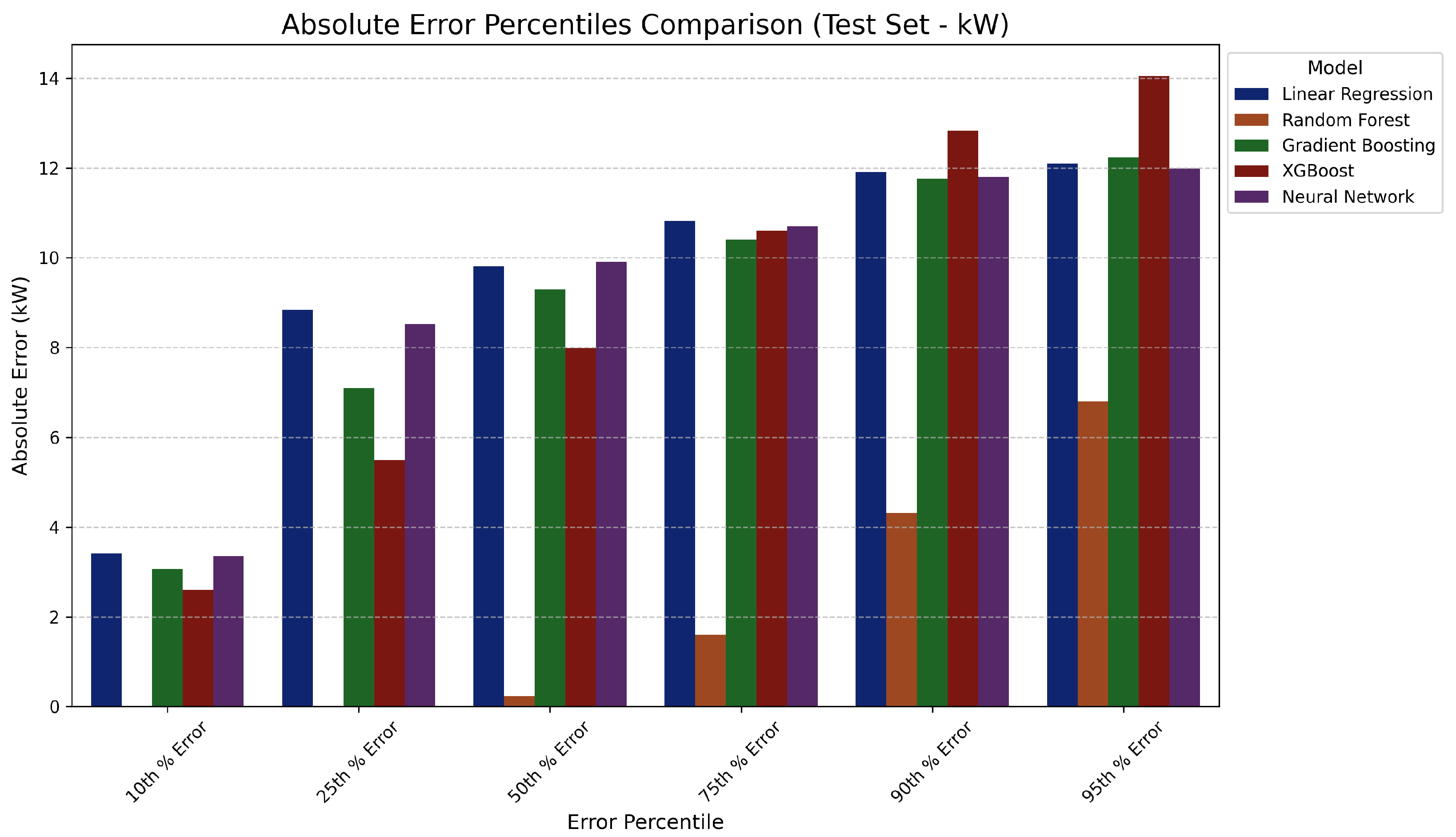
Figure 6 demonstrates that Random Forest and XGBoost maintained substantially lower absolute errors throughout all percentiles compared to other models. Both models showed particularly strong performance at higher percentiles (90th and 95th), indicating reliable prediction even for more challenging cases. Linear Regression and Neural Network exhibited progressively larger errors across percentiles, with the highest errors occurring at extreme percentiles.
All models exhibited non-normal residual distributions. Preliminary target variable transformations did not consistently improve residual normality or predictive performance across models. Final models were trained on untransformed data.

3.1.6. Computational Performance

Table 16 summarizes training and inference times for all models.
Linear Regression achieved the fastest training (0.0149 s) and inference (0.0013 s) times. XGBoost demonstrated exceptional training efficiency (0.5425 s) compared to Random Forest (14.37 s) and Gradient Boosting (8.13 s). Neural Network exhibited the longest training time (678.21 s). All models demonstrated acceptable inference times for real-time applications, with tree-based methods achieving microsecond-level predictions per sample.

3.1.7. Feature Importance Analysis

Figure 7 illustrates feature importance variations across models. Tree-based models (Random Forest, Gradient Boosting, XGBoost) prioritized Frequency Reference, followed by Humidity. Linear Regression identified UV Index as most significant.
Feature Correlation Analysis
To assess both linear and nonlinear feature-target relationships, Pearson, Spearman rank, and Kendall’s tau correlation coefficients were computed [57,58]. Table 17 presents all three correlation metrics.
Frequency Reference exhibited the strongest correlations across all three metrics (Pearson r = 0.952, Spearman ρ = 0.963, Kendall τ = 0.874), followed by uvIndex. Humidity showed consistent negative correlation across all methods. The high concordance between Pearson, Spearman, and Kendall coefficients indicates predominantly monotonic relationships with minimal complex nonlinearity. The uvIndex showed slightly elevated Spearman correlation ( ρ = 0.758) compared to Pearson (r = 0.740), suggesting mild nonlinear monotonic components in its relationship with the target variable.
Multicollinearity Assessment
Variance Inflation Factor (VIF) analysis (Table 18) showed all features had VIF values below 5, confirming absence of severe multicollinearity that could destabilize model coefficients or introduce redundancy.
Feature Redundancy Assessment
To comprehensively assess feature redundancy beyond VIF analysis, feature-feature correlation matrices were computed using all three metrics (Pearson, Spearman, and Kendall). Figure 8 presents these matrices side-by-side for comparison.
Following established guidelines [45,59], a correlation threshold of |r| > 0.80 was used to identify potentially redundant feature pairs that should be considered for removal. Table 19 summarizes the maximum feature-feature correlations observed across all three metrics.
The Spearman correlation between uvIndex and Air Temperature ( ρ = −0.821) marginally exceeded the 0.80 redundancy threshold, while Pearson (r = −0.780) and Kendall ( τ = −0.613) remained below it. This indicates a strong inverse monotonic relationship, likely reflecting early morning or late afternoon conditions when solar radiation is high but ambient temperature remains moderate. All other feature pairs showed correlations well below 0.80 across all three metrics. The second-highest correlations were between Frequency Reference and Wind Speed (Pearson r = 0.704, Spearman ρ = 0.719, Kendall τ = 0.591).
Despite the Spearman correlation exceeding 0.80, both uvIndex and Air Temperature were retained for model training based on multiple converging lines of evidence: (1) only one of three correlation metrics exceeded the threshold, and only marginally (by 0.021), (2) VIF values for both features remained well below 5 (uvIndex: 2.08, Air Temperature: 2.62) as shown in Table 18, confirming multicollinearity does not substantially destabilize coefficient estimates, (3) uvIndex and Air Temperature represent distinct physical mechanisms—UV radiation directly drives photovoltaic generation while temperature inversely affects panel efficiency through thermal effects on semiconductor materials [60], (4) different model types weighted these features differently (Figure 7), suggesting both contribute unique predictive value, (5) tree-based models can leverage interaction effects between these correlated features to capture conditional relationships [47], and (6) Random Forest and XGBoost, our best-performing models, are inherently robust to moderate multicollinearity through ensemble methods [48].

3.2. Phase 2: Output Power Prediction

This subsection presents the results of predicting pump output power using the frequency predictions from Phase 1 as input.

3.2.1. Comparative Model Metrics Across Datasets

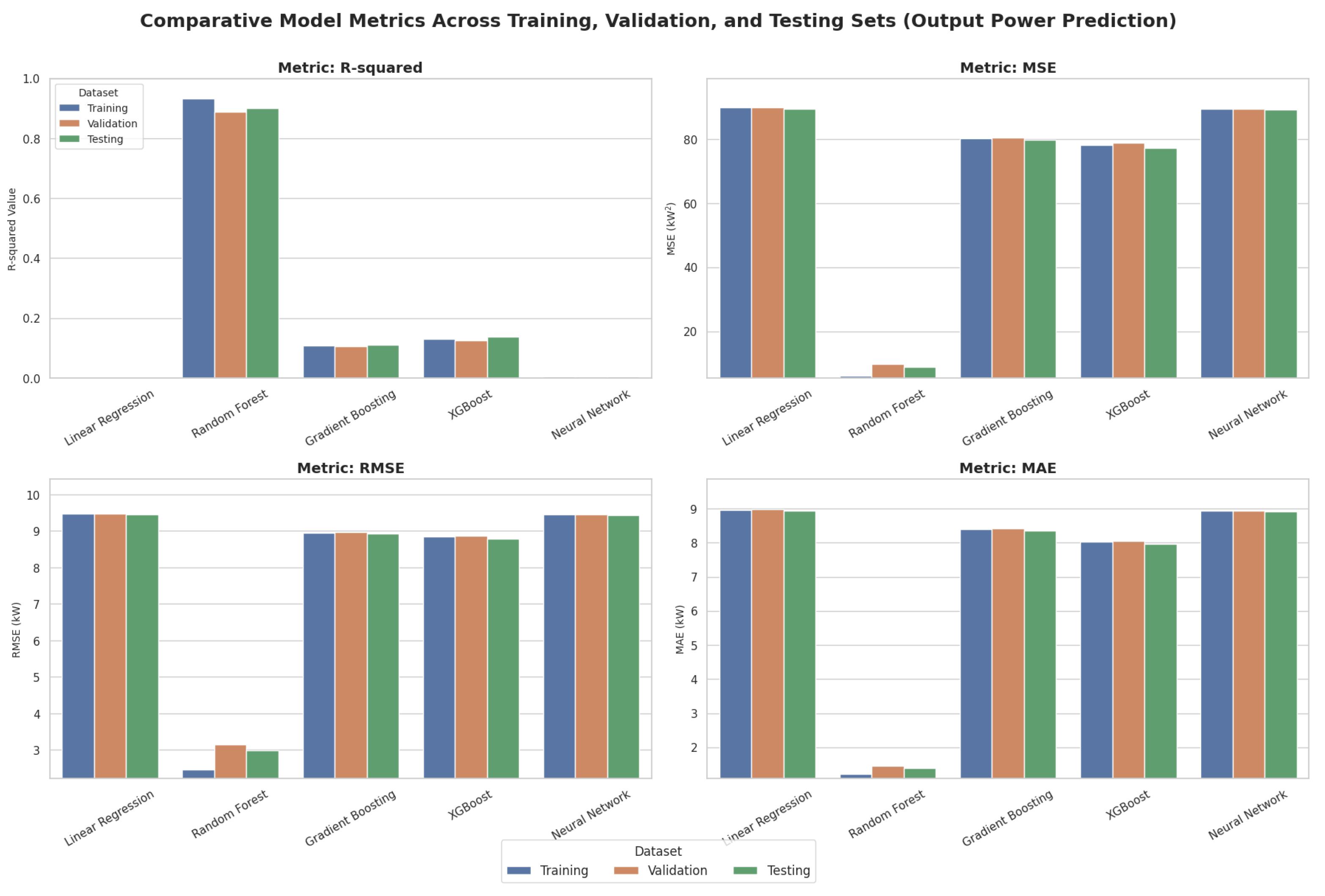
Figure 9 presents model comparisons for output power prediction across all datasets. Random Forest (orange bars) exhibited significantly stronger performance with R-squared values around 0.9 for validation and testing, and dramatically lower error metrics across all datasets. Linear Regression, Gradient Boosting, XGBoost, and Neural Network showed R-squared values near zero with substantially higher errors.

3.2.2. Model Performance Summary

To ensure robustness, all reported metrics (RMSE, MAE, R 2 ) are the mean outcome across ten independent training and evaluation runs, each utilizing a unique random seed for data splitting and model initialization. The Random Forest Regressor demonstrated superior performance, achieving a mean Test RMSE of 2.98 kW (Std Dev: 0.054, 95% CI: [2.87, 3.09]) and a mean Test MAE of 1.39 kW (Std Dev: 0.024, 95% CI: [1.35, 1.44]). This superior performance was coupled with a Test MSE of 8.89, and Test R-squared of 0.9007 (Table 20, Table 21, Table 22, Table 23 and Table 24).
The Persistence Baseline showed the worst performance (Test RMSE 9.41 kW, Test MAE 8.91 kW, Test R2 0.0000).
XGBoost achieved Test RMSE 8.79 kW and Test MAE 7.97 kW. Gradient Boosting obtained Test RMSE 8.92 kW and Test MAE 8.36 kW. Neural Network (NN2) showed Test RMSE 9.44 kW, Test MAE 8.92 kW, Test R2 0.0051. Linear Regression achieved Test RMSE 9.46 kW, Test MAE 8.94 kW, Test R2 0.0007.

3.2.3. Statistical Significance Testing

Wilcoxon Signed-Rank tests confirmed statistically significant differences (p-values 0.001 ) between Random Forest and all other models (Table 25 and Table 26).

3.2.4. Prediction Accuracy Visualization

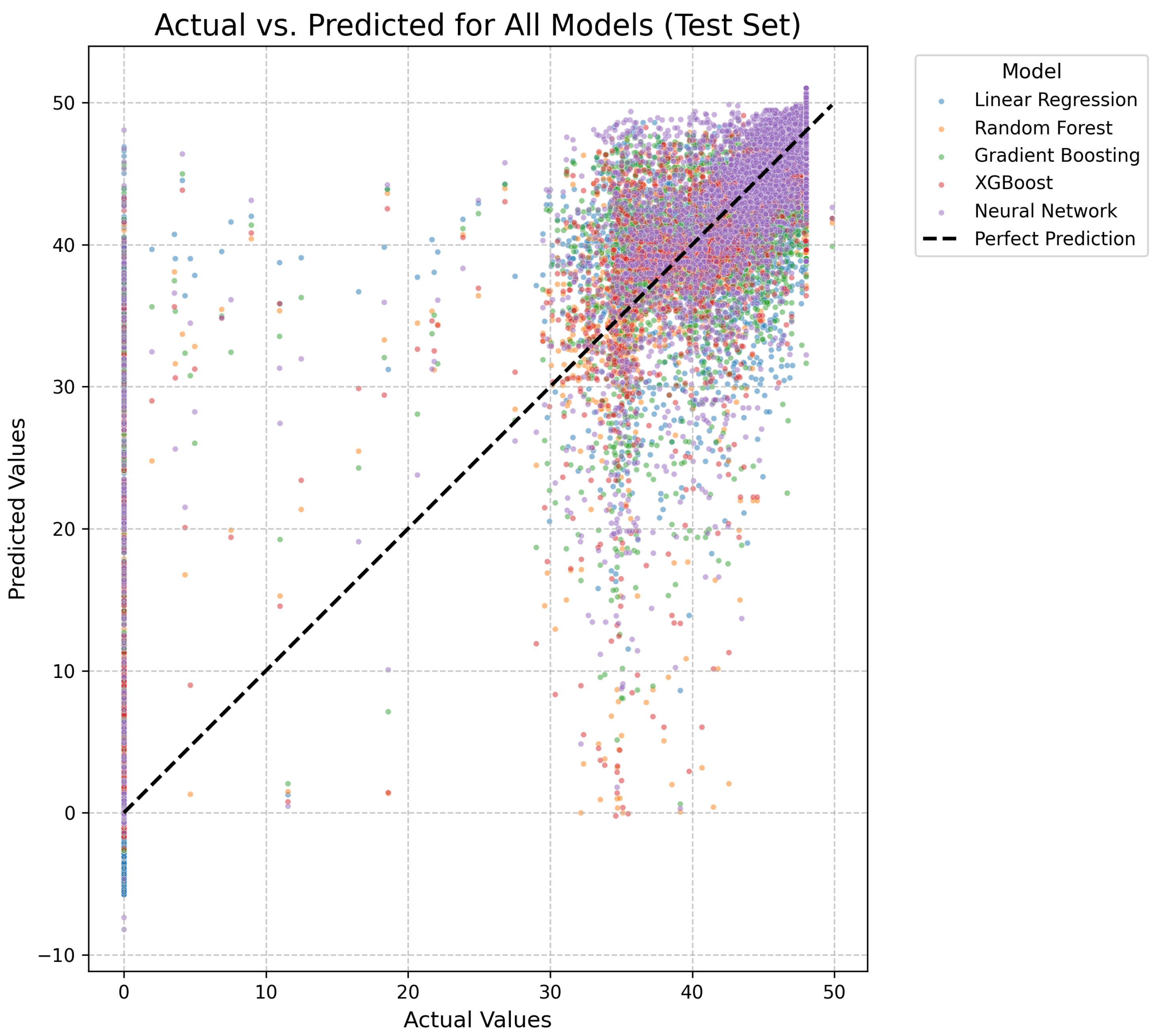
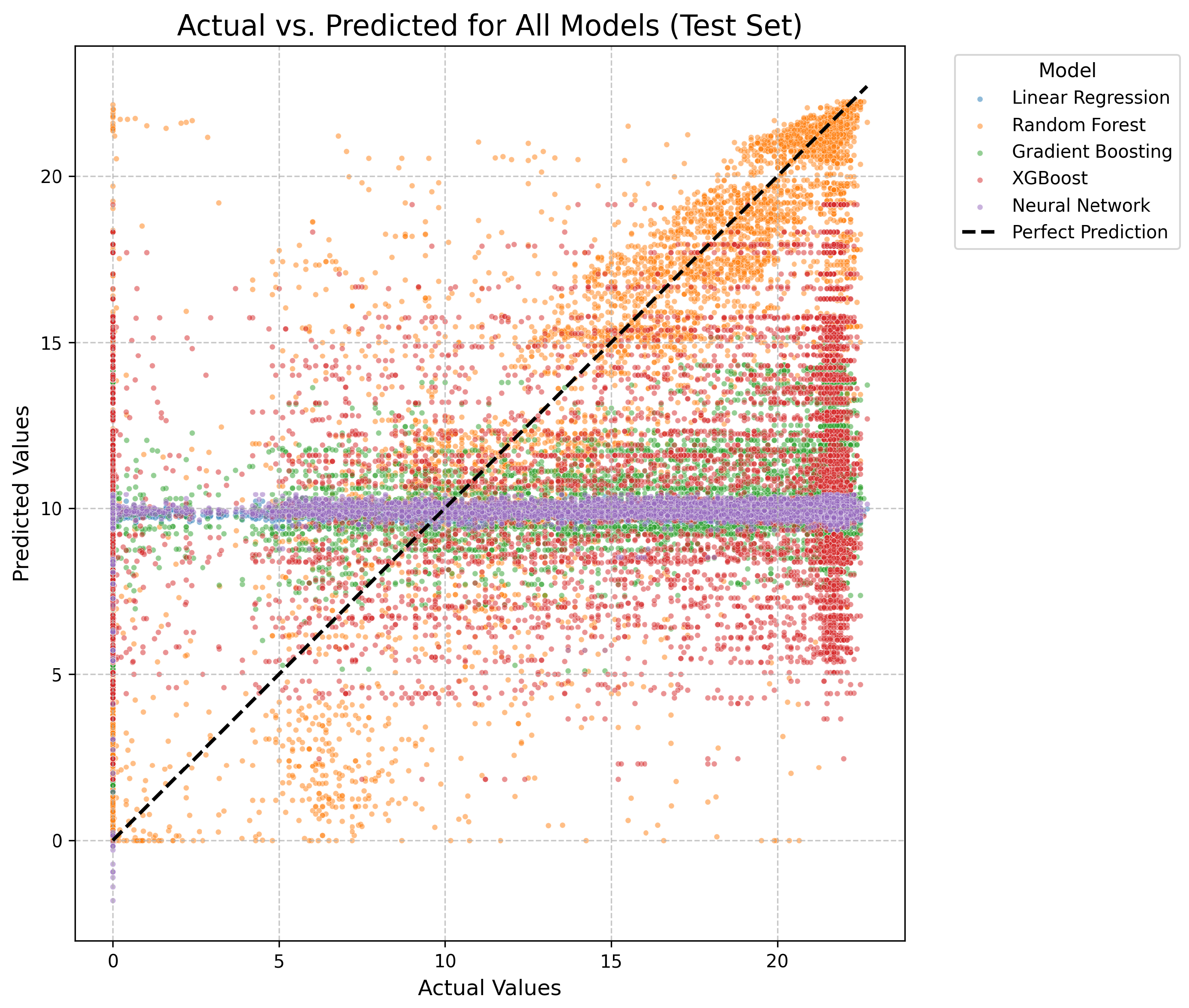
Figure 10 displays actual versus predicted output power values. Random Forest predictions (orange points) formed a tight cluster aligned with the diagonal line. Linear Regression (blue), Gradient Boosting (green), XGBoost (red), and Neural Network (purple) showed highly scattered patterns far from the diagonal.

3.2.5. Error Distribution Analysis

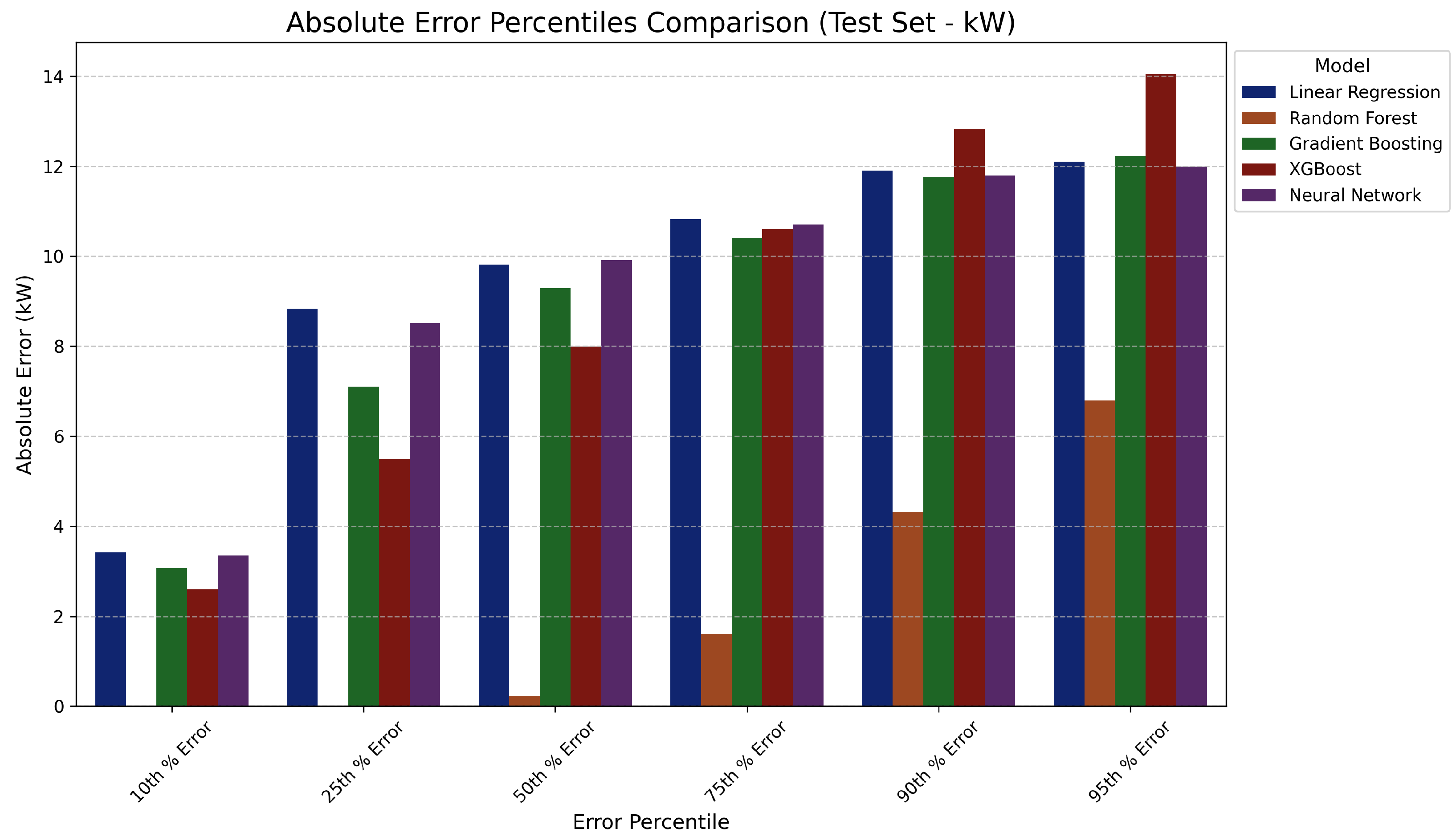
Figure 11 demonstrates Random Forest (brown bars) maintained significantly lower absolute errors throughout all percentiles (10th to 95th) compared to other models. Other models showed substantially higher and more uniform error distributions across percentiles.
All models exhibited non-normal residual distributions. Preliminary target variable transformations did not consistently improve residual normality or predictive performance. Final models were trained on untransformed data.

3.2.6. Computational Performance

Table 27 presents training and inference times for Phase 2.
Linear Regression was fastest for both training and inference. XGBoost demonstrated exceptional training efficiency (0.44 s) compared to Random Forest (27.24 s) and Gradient Boosting (5.22 s). Neural Network required the longest training time (828.26 s). All models demonstrated acceptable inference times for real-time applications.

3.3. Annual Water Volume Distribution

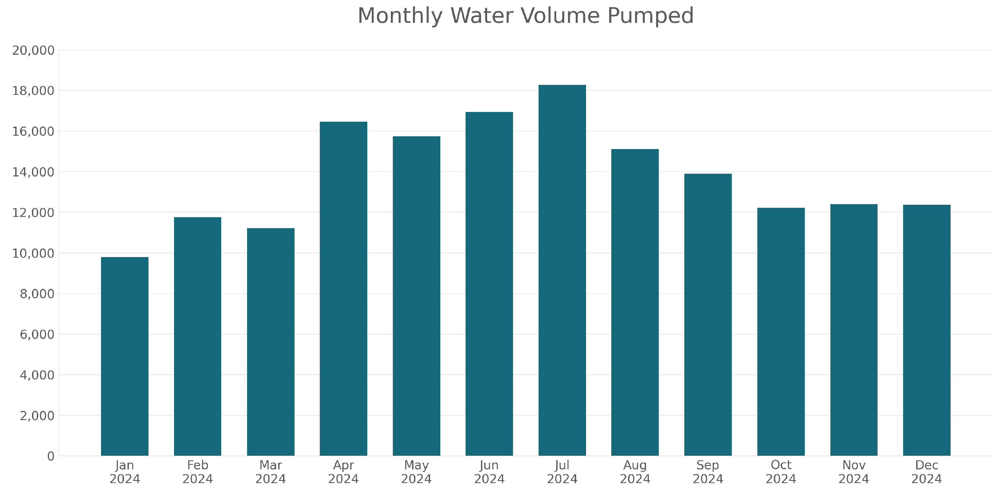
The dataset was extended using the two-phase Random Forest framework. By applying both models to an additional six months of data, a complete one-year dataset was constructed. Monthly water volumes were computed and are presented in Table 28.
The highest water volume was pumped in July (18,276.96 m3 = 18,276,960 L), while the lowest occurred in January (9784.20 m3 = 9,784,200 L). The total annual water volume pumped was 166,132.77 m3 (166,132,770 L).
Figure 12 displays the monthly water volume distribution pattern, showing peak volumes during summer months and reduced volumes during winter months.

4. Discussion

This section interprets the results presented in Section 3, examining the implications of model performance, exploring practical significance, and contextualizing findings within the broader field of machine learning applications for inverter-driven pump systems.

4.1. Output Frequency Prediction Analysis

This subsection discusses the results of predicting inverter motor output frequency from environmental conditions.

4.1.1. Model Performance and Generalization

The Random Forest and XGBoost models demonstrated excellent generalization across training, validation, and testing datasets, as evidenced by Figure 4. The strong performance on validation and test sets, despite higher R-squared values on training data, indicates these models successfully captured underlying patterns without substantial overfitting. This robustness is particularly valuable for real-world deployment where model reliability across diverse operating conditions is essential.
The Neural Network’s discernible performance gap between training and validation/testing sets, despite Bayesian optimization, suggests that the architecture may have been limited in capturing the specific non-linear relationships present in this dataset, or that the model was sensitive to initialization and hyperparameter choices. This highlights a key advantage of tree-based ensemble methods for tabular data: they often achieve superior performance with less extensive hyperparameter tuning compared to deep learning approaches.

4.1.2. Practical Significance of Prediction Errors

The Random Forest model’s test RMSE of 3.28 Hz and MAE of 1.00 Hz represent small deviations within typical industrial pump operating ranges (20–120 Hz). These errors indicate high predictive accuracy with practical operational relevance. Given that industrial pumps operate within this frequency range, errors of this magnitude suggest that the model can reliably predict operating conditions with minimal deviation from expected performance.
Accurate frequency prediction is particularly critical because it serves as a crucial input for Phase 2 power prediction. Minimizing errors in Phase 1 directly enhances the reliability of subsequent power predictions, creating a cascading effect on overall system accuracy. The error percentile analysis (Figure 6) demonstrates that Random Forest and XGBoost maintained substantially lower errors throughout all percentiles, with particularly strong performance at the 90th and 95th percentiles. While occasional larger errors (up to approximately 8 Hz) occur at extreme percentiles, the overall predictive performance remains within practical limits.

4.1.3. Feature Importance Discrepancies and Model Interpretability

The substantial differences in feature importance across model types (Figure 7) reflect fundamental differences in how models capture data relationships. Tree-based models consistently prioritized Frequency Reference and Humidity, while Linear Regression identified UV Index as most significant. This discrepancy arises from distinct modeling strategies for capturing underlying relationships.
The comprehensive correlation analysis (Table 17) revealed that Frequency Reference exhibits the strongest relationship with output frequency across all three metrics (Pearson r = 0.952, Spearman ρ = 0.963, Kendall τ = 0.874), validating its role as the primary control parameter. This explains why all model types recognize its importance. For uvIndex, the slightly elevated Spearman correlation ( ρ = 0.758) compared to Pearson (r = 0.740) suggests mild nonlinear monotonic components, which tree-based models can exploit through their recursive partitioning strategy while Linear Regression captures the strong linear association.
The VIF analysis (Table 18) confirmed that multicollinearity is moderate and unlikely to destabilize model coefficients, with all features exhibiting VIF values below 5. The comprehensive correlation analysis using three metrics (Pearson, Spearman, and Kendall) provided additional evidence that feature importance discrepancies stem from modeling approach differences rather than problematic multicollinearity or feature redundancy issues.
These findings underscore an important principle: linear models emphasize direct linear associations, while tree-based models capture complex, non-linear dynamics. Using multiple model types provides a more comprehensive understanding of feature contributions in complex systems. The tree-based models’ ability to capture these non-linear patterns likely explains their superior predictive performance in this application.
Nonlinear Correlation and Feature Redundancy
Comprehensive correlation analysis using Pearson, Spearman, and Kendall metrics (Table 17, Figure 8) revealed predominantly monotonic relationships with high concordance across methods. Only uvIndex–Air Temperature Spearman correlation ( ρ = −0.821) exceeded the 0.80 redundancy threshold, while Pearson (r = −0.780) and Kendall ( τ = −0.613) remained below threshold (Table 19).
The decision to retain both features despite this threshold exceedance is justified by six converging lines of evidence: (1) only one of three metrics marginally exceeded threshold (by 0.021), as conservative approaches recommend removal only when multiple metrics consistently exceed thresholds [59], (2) VIF values well below 5 (uvIndex: 2.08, Air Temperature: 2.62) confirming manageable multicollinearity [46,61], (3) distinct physical mechanisms—UV drives photovoltaic generation while temperature affects thermal efficiency [60,62]—representing independent causal pathways despite observational correlation, (4) differential model importance patterns (Figure 7) indicating both features provide complementary information, (5) interaction effects enabling tree-based models to distinguish optimal conditions (high UV, moderate temperature) from thermal-loss scenarios (high UV, high temperature) [47], and (6) ensemble method robustness to moderate multicollinearity through bootstrap aggregation and feature subsampling [48].
This multi-criteria assessment demonstrates that threshold exceedance alone does not warrant removal when comprehensive evidence supports retention. All other feature pairs remained well below 0.80 across all metrics, confirming minimal redundancy. The exceptionally high Frequency Reference correlation (r = 0.952, ρ = 0.963, τ = 0.874) reflects deterministic control relationships supported by domain knowledge [37] rather than spurious associations.

4.1.4. Computational Efficiency Considerations

The computational performance analysis (Table 16) reveals important trade-offs between accuracy and computational cost. Linear Regression’s minimal training (0.0149 s) and inference (0.0013 s) times reflect its mathematical simplicity, but this comes at the cost of predictive accuracy.
XGBoost’s exceptional training efficiency (0.5425 s) while maintaining competitive accuracy makes it particularly attractive. Random Forest’s longer training time (14.37 s) is justified by its superior predictive accuracy. For low-latency predictions, all models except the Neural Network demonstrate acceptable inference times, with tree-based methods achieving microsecond-level predictions per sample.
The Neural Network’s lengthy training time (678.21 s) without corresponding performance benefits highlights that deep learning approaches may not be optimal for all tabular data problems.

4.2. Output Power Prediction Analysis

The following analysis examines model performance in predicting pump output power.

4.2.1. Performance Differences Between Models

The Phase 2 results revealed substantial performance disparities, with Random Forest demonstrating markedly superior performance compared to competing models. While Random Forest achieved Test R2 of 0.9007, other models showed R2 values near zero, essentially performing no better than the persistence baseline. This dramatic difference warrants careful interpretation.
The poor performance of Linear Regression, Neural Network, and even gradient boosting methods (despite their moderate success in Phase 1) suggests that the relationship between input features (including predicted frequency from Phase 1) and output power is highly non-linear and complex. Random Forest’s ability to model intricate interactions through its ensemble of decision trees appears uniquely suited to capture these relationships.

4.2.2. Practical Significance for Industrial Applications

For the pump’s operational range of 0–25 kW, Random Forest’s Test RMSE of 2.98 kW and MAE of 1.39 kW correspond to relative errors of approximately 11.9% and 5.6%, respectively. These errors are acceptable for flow estimation and system monitoring applications.
Output power prediction serves as a reliable proxy for water volume estimation because of the strong correlation between power, flow rate, head, and pump efficiency. Accurate predictions support real-time pump operation by enabling flow estimation without additional sensors.
The error percentile analysis (Figure 11) demonstrates that Random Forest maintained significantly lower errors throughout all percentiles compared to other models. This concentration of small errors is more important than occasional outliers, as it indicates reliable day-to-day performance.

4.2.3. Why Other Models Failed in Phase 2

The failure of models that performed reasonably in Phase 1 requires explanation. Several factors may contribute:
  • Increased Complexity: The relationship between environmental factors and output power may involve more complex interactions than the frequency prediction task. Power depends not only on frequency but also on load conditions, efficiency curves, and other non-linear dependencies.
  • Error Propagation: Phase 2 models receive predicted frequency from Phase 1 as input rather than true frequency values. Any prediction errors from Phase 1 cascade into Phase 2, potentially amplifying errors for models less robust to input noise.
  • Model Architecture Limitations: Linear models inherently cannot capture complex non-linear relationships. The Neural Network’s failure despite its theoretical capacity for non-linear modeling suggests inadequate architecture or poor hyperparameter tuning for this specific problem.
  • Random Forest’s Advantage: Random Forest’s ensemble approach with bootstrap aggregating may provide superior robustness to noisy inputs and enhanced ability to model complex interaction effects compared to single-tree or linear approaches.

4.2.4. Computational Trade-Offs in Phase 2

Random Forest’s training time (27.24 s) is longer than XGBoost (0.44 s) but substantially shorter than the Neural Network (828.26 s). Given Random Forest’s vastly superior accuracy, this moderate computational cost represents an excellent trade-off. The model’s inference time remains acceptable for real-time applications.
For scenarios requiring frequent model updates, the computational cost must be weighed against accuracy requirements.

4.3. Deployment Feasibility in Resource-Constrained Desert Environments

In remote desert regions, edge deployment of AI models is constrained by limited access to grid electricity, reliance on solar power, and average hardware capabilities (e.g., microcontrollers or low-power embedded systems). While deep learning models such as neural networks offer flexibility, their high training time (e.g., 678.21 s in Phase 1 and 828.26 s in Phase 2) and memory requirements make them less suitable for real-time deployment on low-power devices. In contrast, tree-based models, particularly Random Forest, demonstrate a favorable trade-off between accuracy and computational cost. With microsecond-level inference times and minimal memory overhead, Random Forest can be deployed on devices such as Raspberry Pi or NVIDIA Jetson Nano, which are commonly used on solar-powered agricultural setups. Moreover, its robustness to noisy inputs and low-energy consumption during inference make it ideal for continuous operation in harsh environments. These considerations reinforce our choice of Random Forest as the preferred model for practical deployment in resource-constrained settings.

4.4. Water Volume Analysis and Seasonal Patterns

The annual water volume distribution analysis (Table 28 and Figure 12) demonstrates clear seasonal patterns that align with Egyptian climate conditions. Peak pumping in July (18,276.96 m3) corresponds to maximum summer irrigation demands and evapotranspiration rates, while minimum pumping in January (9784.20 m3) reflects reduced winter crop water requirements.
This seasonal variation serves two important purposes: (1) it validates the practical applicability of the developed predictive framework for agricultural water management planning, demonstrating that predictions capture real-world operational patterns, and (2) it provides actionable insights for resource allocation and energy management strategies aligned with seasonal demand patterns.
The total annual volume of 166,132.77 m3 provides a baseline for planning future irrigation needs and assessing system capacity.

4.5. Summary of Discussion

The results demonstrate that machine learning, particularly Random Forest models, can effectively predict both output frequency and output power in inverter-driven pump systems. The two-phase framework achieved high accuracy while maintaining computational efficiency suitable for practical deployment. The performance differences between models—especially in Phase 2—underscore the importance of careful model selection and validation rather than relying on default approaches.
The successful application to annual water volume estimation validates the practical utility of the framework for agricultural water management. The clear seasonal patterns captured by predictions align with known climatic variations, demonstrating that models capture physically meaningful relationships rather than spurious correlations.
These findings contribute to the growing body of evidence.

5. Conclusions

This study developed an AI-powered Digital Twin framework to optimize a solar-powered submersible pump system in the Khataba region, Elsadat, Beheira Governorate, Egypt. Using a six-month dataset of environmental and inverter motor data, the framework employed a two-phase machine learning approach to predict system performance.
The framework operates in two phases: Phase 1 predicts the inverter motor’s output frequency from environmental inputs (UV index, air temperature, wind speed, humidity), and Phase 2 estimates pump output power using the predicted frequency. Multiple machine learning models were evaluated including Linear Regression, Random Forest, Gradient Boosting, XGBoost, and Neural Networks.
The Random Forest model demonstrated superior predictive performance in both phases, achieving Test MAE of 1.00 Hz and RMSE of 3.28 Hz in Phase 1, and Test MAE of 1.39 kW and RMSE of 2.98 kW in Phase 2. These results highlight Random Forest’s capacity to model complex, nonlinear relationships between environmental conditions and system behavior.
The framework successfully estimated annual water delivery of 166,132.77 m3, with peak monthly output of 18,276.96 m3 in July and minimum of 9784.20 m3 in January. These seasonal patterns align with Egyptian climate conditions and irrigation demands, validating the practical utility of the framework for agricultural water management planning.
The dramatic performance differences between models—especially in Phase 2 where Random Forest achieved R2 of 0.9007 while other models approached zero—underscore the importance of careful model selection rather than relying on default approaches. The staged two-phase approach proved more effective than attempting direct power prediction from environmental variables alone.

Future Work

While the proposed framework demonstrates strong predictive performance, the dataset used in this study was collected over a six-month period from a single geographic location (Khataba, Egypt). This temporal and spatial limitation may affect the generalizability of the model to other regions with different climatic conditions or seasonal patterns. Future work should explore cross-seasonal validation using extended datasets that span multiple years and diverse geographic locations. Additionally, synthetic data augmentation techniques, such as generative modeling or domain adaptation, could be employed to simulate environmental variability and enhance model robustness across broader deployment scenarios. Moreover, if the dataset is significantly extended over a longer temporal duration, exploring larger, more complex models—such as advanced deep learning architectures or transformer models—may yield further performance gains.
Moreover, to evolve the proposed framework into a fully adaptive digital twin, future implementations should incorporate real-time sensor feedback to enable closed-loop control. For example, flow rate sensors, inverter fault logs, and pump temperature readings can be continuously monitored and fed back into the AI models to refine predictions and trigger corrective actions. This feedback loop would allow the system to dynamically adjust inverter frequency or pump operation in response to anomalies or environmental fluctuations. Such integration supports predictive maintenance, energy-efficient operation, and resilience in harsh desert environments.
Another limitation is the reliability of sensors in harsh desert environments, as dust, heat, and humidity can degrade sensor accuracy or lead to failure. Redundant sensing and periodic calibration may be necessary to maintain data integrity. Also, maintenance of hardware components such as solar panels, inverters, and pumps requires trained personnel and logistic planning, which may not be readily available in all regions. Future work should explore fault-tolerant architectures and self-diagnostic capabilities.

Author Contributions

Conceptualization, M.H., S.I. and O.S.; Methodology, Y.S. and O.S.; Software, Y.S.; Validation, O.S., E.K., S.I. and M.H.; Formal analysis, E.K. and O.S.; Investigation, E.K. and O.S.; Resources, Y.S.; Data curation, M.H. and S.I.; Writing—original draft preparation, Y.S. and O.S.; Writing—review and editing, E.K. and Y.S.; Visualization, E.K., Y.S. and O.S.; Supervision, M.H. and O.S.; Project administration, M.H. and O.S.; Funding acquisition, Not applicable. All authors have read and agreed to the published version of the manuscript.

Funding

This research received no external funding.

Data Availability Statement

The data is available at https://data.mendeley.com/datasets/wgfhmx37ng/1. URL accessed on 1 September 2025.

Acknowledgments

The researchers acknowledge Ajman University for its support in this research.

Conflicts of Interest

The authors declare no conflicts of interest.

References

  1. Yang, Y.; Wang, H.; Wang, C.; Zhou, L.; Ji, L.; Yang, Y.; Shi, W.; Agarwal, R.K. An entropy efficiency model and its application to energy performance analysis of a multi-stage electric submersible pump. Energy 2024, 288, 129741. [Google Scholar] [CrossRef]
  2. Zhou, Q.; Li, H.; Zeng, X.; Li, L.; Cui, S.; Du, Z. A quantitative safety assessment for offshore equipment evaluation using fuzzy FMECA: A case study of the hydraulic submersible pump system. Ocean. Eng. 2024, 293, 116611. [Google Scholar] [CrossRef]
  3. Wei, A.; Wang, W.; Hu, Y.; Feng, S.; Qiu, L.; Zhang, X. Numerical and experimental analysis of the cavitation and flow characteristics in liquid nitrogen submersible pump. Phys. Fluids 2024, 36, 042109. [Google Scholar] [CrossRef]
  4. Salah, Y.; Shalash, O.; Khatab, E. A lightweight speaker verification approach for autonomous vehicles. Robot. Integr. Manuf. Control 2024, 1, 15–30. [Google Scholar] [CrossRef]
  5. García, J.A.; Asuaje, M.; Pereyra, E.; Ratkovich, N. Analysis of two-phase gas-liquid flow in an Electric Submersible Pump using A CFD approach. Geoenergy Sci. Eng. 2024, 233, 212510. [Google Scholar] [CrossRef]
  6. Yang, C.; Xu, Q.; Chang, L.; Dai, X.; Wang, H.; Su, X.; Guo, L. Interstage performance and power consumption of a multistage mixed-flow electrical submersible pump in gas–liquid conditions: An experimental study. J. Fluids Eng. 2024, 146, 051203. [Google Scholar] [CrossRef]
  7. Elkholy, M.; Shalash, O.; Hamad, M.S.; Saraya, M. Harnessing Machine Learning for Effective Energy Theft Detection Based on Egyptian Data. In Proceedings of the International Conference on Energy Systems, Istanbul, Turkey, 12–14 May 2025. [Google Scholar]
  8. Cui, B.; Chen, H.; Zhu, Z.; Sun, L.; Sun, L. Optimization of low-temperature multi-stage submersible pump based on blade load. Phys. Fluids 2024, 36, 035157. [Google Scholar] [CrossRef]
  9. Ahmadizadeh, M.; Heidari, M.; Thangavel, S.; Al Naamani, E.; Khashehchi, M.; Verma, V.; Kumar, A. Technological advancements in sustainable and renewable solar energy systems. In Highly Efficient Thermal Renewable Energy Systems; CRC Press: Boca Raton, FL, USA, 2024; pp. 23–39. [Google Scholar]
  10. Elkholy, M.; Shalash, O.; Hamad, M.S.; Saraya, M.S. Empowering the grid: A comprehensive review of artificial intelligence techniques in smart grids. In Proceedings of the 2024 International Telecommunications Conference (ITC-Egypt), Cairo, Egypt, 22–25 July 2024; pp. 513–518. [Google Scholar]
  11. Tripathi, A.K.; Aruna, M.; Elumalai, P.; Karthik, K.; Khan, S.A.; Asif, M.; Rao, K.S. Advancing solar PV panel power prediction: A comparative machine learning approach in fluctuating environmental conditions. Case Stud. Therm. Eng. 2024, 59, 104459. [Google Scholar] [CrossRef]
  12. Sun, Y.; Usman, M.; Radulescu, M.; Pata, U.K.; Balsalobre-Lorente, D. New insights from the STIPART model on how environmental-related technologies, natural resources and the use of the renewable energy influence load capacity factor. Gondwana Res. 2024, 129, 398–411. [Google Scholar] [CrossRef]
  13. Xu, G.; Yang, M.; Li, S.; Jiang, M.; Rehman, H. Evaluating the effect of renewable energy investment on renewable energy development in China with panel threshold model. Energy Policy 2024, 187, 114029. [Google Scholar] [CrossRef]
  14. Fawzy, H.; Elbrawy, A.; Amr, M.; Eltanekhy, O.; Khatab, E.; Shalash, O. A systematic review: Computer vision algorithms in drone surveillance. J. Robot. Integr. 2025. [Google Scholar] [CrossRef]
  15. Li, B.; Amin, A.; Nureen, N.; Saqib, N.; Wang, L.; Rehman, M.A. Assessing factors influencing renewable energy deployment and the role of natural resources in MENA countries. Resour. Policy 2024, 88, 104417. [Google Scholar] [CrossRef]
  16. Shahzad, U.; Tiwari, S.; Mohammed, K.S.; Zenchenko, S. Asymmetric nexus between renewable energy, economic progress, and ecological issues: Testing the LCC hypothesis in the context of sustainability perspective. Gondwana Res. 2024, 129, 465–475. [Google Scholar] [CrossRef]
  17. Yasser, M.; Shalash, O.; Ismail, O. Optimized decentralized swarm communication algorithms for efficient task allocation and power consumption in swarm robotics. Robotics 2024, 13, 66. [Google Scholar] [CrossRef]
  18. Gaber, I.M.; Shalash, O.; Hamad, M.S. Optimized inter-turn short circuit fault diagnosis for induction motors using neural networks with leleru. In Proceedings of the 2023 IEEE Conference on Power Electronics and Renewable Energy (CPERE), Luxor, Egypt, 19–21 February 2023; pp. 1–5. [Google Scholar]
  19. Khatab, E.; Onsy, A.; Abouelfarag, A. Evaluation of 3D vulnerable objects’ detection using a multi-sensors system for autonomous vehicles. Sensors 2022, 22, 1663. [Google Scholar] [CrossRef]
  20. Shalash, O.; MÃl’twalli, A.; Sallam, M.H.; Khatab, E. High-Performance Polygraph-Based Truth Detection System: Leveraging Multi-Modal Data Fusion and Particle Swarm-Optimized Random Forest for Robust Deception Analysis. Authorea 2025. [Google Scholar] [CrossRef]
  21. Khatab, E.; Onsy, A.; Varley, M.; Abouelfarag, A. A lightweight network for real-time rain streaks and rain accumulation removal from single images captured by avs. Appl. Sci. 2022, 13, 219. [Google Scholar] [CrossRef]
  22. Said, H.; Mohamed, S.; Shalash, O.; Khatab, E.; Aman, O.; Shaaban, R.; Hesham, M. Forearm Intravenous Detection and Localization for Autonomous Vein Injection Using Contrast-Limited Adaptive Histogram Equalization Algorithm. Appl. Sci. 2024, 14, 7115. [Google Scholar] [CrossRef]
  23. Khaled, A.; Shalash, O.; Ismaeil, O. Multiple objects detection and localization using data fusion. In Proceedings of the 2023 2nd International Conference on Automation, Robotics and Computer Engineering (ICARCE), Wuhan, China, 14–16 December 2023; pp. 1–6. [Google Scholar]
  24. Elsayed, H.; Tawfik, N.S.; Shalash, O.; Ismail, O. Enhancing human emotion classification in human-robot interaction. In Proceedings of the 2024 International Conference on Machine Intelligence and Smart Innovation (ICMISI), Alexandria, Egypt, 12–14 May 2024; pp. 1–6. [Google Scholar]
  25. Métwalli, A.; Shalash, O.; Elhefny, A.; Rezk, N.; El Gohary, F.; El Hennawy, O.; Akrab, F.; Shawky, A.; Mohamed, Z.; Hassan, N.; et al. Enhancing hydroponic farming with Machine Learning: Growth prediction and anomaly detection. Eng. Appl. Artif. Intell. 2025, 157, 111214. [Google Scholar] [CrossRef]
  26. Issa, R.; Badr, M.M.; Shalash, O.; Othman, A.A.; Hamdan, E.; Hamad, M.S.; Abdel-Khalik, A.S.; Ahmed, S.; Imam, S.M. A data-driven digital twin of electric vehicle Li-ion battery state-of-charge estimation enabled by driving behavior application programming interfaces. Batteries 2023, 9, 521. [Google Scholar] [CrossRef]
  27. Alao, K.T.; Gilani, S.I.U.H.; Sopian, K.; Alao, T.O. A review on digital twin application in photovoltaic energy systems: Challenges and opportunities. JMST Adv. 2024, 6, 257–282. [Google Scholar] [CrossRef]
  28. Shalash, O.; Rowe, P. Computer-assisted robotic system for autonomous unicompartmental knee arthroplasty. Alex. Eng. J. 2023, 70, 441–451. [Google Scholar] [CrossRef]
  29. Olayiwola, O.; Cali, U.; Elsden, M.; Yadav, P. Enhanced Solar Photovoltaic System Management and Integration: The Digital Twin Concept. Solar 2025, 5, 7. [Google Scholar] [CrossRef]
  30. Alshireedah, A.; Yusupov, Z.; Rahebi, J. Optimizing Solar Water-Pumping Systems Using PID-Jellyfish Controller with ANN Integration. Electronics 2025, 14, 1172. [Google Scholar] [CrossRef]
  31. Sumathi, S.; Abitha, S. A novel method for solar water pumping system using machine learning techniques. Proc. Aip Conf. 2023, 2901, 070001. [Google Scholar]
  32. Don, M.G.; Liyanarachchi, S.; Wanasinghe, T.R. A digital twin development framework for an electrical submersible pump (ESP). Arch. Adv. Eng. Sci. 2025, 3, 35–43. [Google Scholar] [CrossRef]
  33. Cheacharoen, R.; Boyd, C.C.; Burkhard, G.F.; Leijtens, T.; Raiford, J.A.; Bush, K.A.; Bent, S.F.; McGehee, M.D. Encapsulating perovskite solar cells to withstand damp heat and thermal cycling. Sustain. Energy Fuels 2018, 2, 2398–2406. [Google Scholar] [CrossRef]
  34. Jordan, D.C.; Kurtz, S.R. Photovoltaic degradation rates—an analytical review. Prog. Photovolt. Res. Appl. 2013, 21, 12–29. [Google Scholar] [CrossRef]
  35. Hudișteanu, V.S.; Cherecheș, N.C.; Țurcanu, F.E.; Hudișteanu, I.; Romila, C. Impact of temperature on the efficiency of monocrystalline and polycrystalline photovoltaic panels: A comprehensive experimental analysis for sustainable energy solutions. Sustainability 2024, 16, 10566. [Google Scholar] [CrossRef]
  36. Hudișteanu, S.V.; Țurcanu, F.E.; Cherecheș, N.C.; Popovici, C.G.; Verdeș, M.; Huditeanu, I. Enhancement of PV panel power production by passive cooling using heat sinks with perforated fins. Appl. Sci. 2021, 11, 11323. [Google Scholar] [CrossRef]
  37. Rabaia, M.K.H.; Abdelkareem, M.A.; Sayed, E.T.; Elsaid, K.; Chae, K.J.; Wilberforce, T.; Olabi, A. Environmental impacts of solar energy systems: A review. Sci. Total Environ. 2021, 754, 141989. [Google Scholar] [CrossRef]
  38. Salah, Y.; Shalash, O.; Khatab, E.; Imam, S.; Hamad, M. Dataset for Solar-Powered Submersible Pump Systems. 2025. Available online: https://data.mendeley.com/datasets/wgfhmx37ng/1 (accessed on 9 September 2025).
  39. Rubin, D.B. Inference and missing data. Biometrika 1976, 63, 581–592. [Google Scholar] [CrossRef]
  40. Little, R.J.; Rubin, D.B. Statistical Analysis with Missing Data, 3rd ed.; John Wiley & Sons: Hoboken, NJ, USA, 2019. [Google Scholar]
  41. Géron, A. Hands-On Machine Learning with Scikit-Learn, Keras, and TensorFlow; O’Reilly Media: Sebastopol, CA, USA, 2019. [Google Scholar]
  42. Goodfellow, I.; Bengio, Y.; Courville, A. Deep Learning; MIT Press: Cambridge, MA, USA, 2016. [Google Scholar]
  43. Hastie, T.; Tibshirani, R.; Friedman, J. The Elements of Statistical Learning: Data Mining, Inference, and Prediction; Springer: Berlin/Heidelberg, Germany, 2009. [Google Scholar]
  44. Bishop, C.M. Pattern Recognition and Machine Learning; Springer: Berlin/Heidelberg, Germany, 2006. [Google Scholar]
  45. Kuhn, M.; Johnson, K. Applied Predictive Modeling; Springer: Berlin/Heidelberg, Germany, 2013. [Google Scholar]
  46. James, G.; Witten, D.; Hastie, T.; Tibshirani, R. An Introduction to Statistical Learning: With Applications in R; Springer: Berlin/Heidelberg, Germany, 2013. [Google Scholar]
  47. Breiman, L. Random forests. Mach. Learn. 2001, 45, 5–32. [Google Scholar] [CrossRef]
  48. Chen, T.; Guestrin, C. XGBoost: A Scalable Tree Boosting System. In Proceedings of the 22nd ACM SIGKDD International Conference on Knowledge Discovery and Data Mining, San Francisco, CA, USA, 13–17 August 2016; pp. 785–794. [Google Scholar]
  49. Friedman, J.H. Greedy function approximation: A gradient boosting machine. Ann. Stat. 2001, 29, 1189–1232. [Google Scholar] [CrossRef]
  50. Seber, G.A.F.; Lee, A.J. Linear Regression Analysis; Wiley: Hoboken, NJ, USA, 2012. [Google Scholar]
  51. Nair, V.; Hinton, G.E. Rectified linear units improve restricted boltzmann machines. In Proceedings of the 27th International Conference on Machine Learning (ICML-10), Haifa, Israel, 21–24 June 2010; pp. 807–814. [Google Scholar]
  52. Kingma, D.P.; Ba, J. Adam: A method for stochastic optimization. In Proceedings of the International Conference on Learning Representations (ICLR), San Diego, CA, USA, 7–9 May 2015. [Google Scholar]
  53. Friedman, J.H. Stochastic gradient boosting. Comput. Stat. Data Anal. 2002, 38, 367–378. [Google Scholar] [CrossRef]
  54. Elrefai, M.; Hamdy, R.A.; ElZawawi, A.; Hamad, M.S. Design and performance evaluation of a solar water pumping system: A case study. In Proceedings of the 2016 Eighteenth International Middle East Power Systems Conference (MEPCON), Cairo, Egypt, 27–29 December 2016; pp. 914–920. [Google Scholar]
  55. Chai, T.; Draxler, R.R. Root mean square error (RMSE) or mean absolute error (MAE)?—Arguments against avoiding RMSE in the literature. Geosci. Model Dev. 2014, 7, 1247–1250. [Google Scholar] [CrossRef]
  56. Montgomery, D.C.; Peck, E.A.; Vining, G.G. Introduction to Linear Regression Analysis, 5th ed.; John Wiley & Sons: Hoboken, NJ, USA, 2012. [Google Scholar]
  57. Spearman, C. The proof and measurement of association between two things. Am. J. Psychol. 1904, 15, 72–101. [Google Scholar] [CrossRef]
  58. Kendall, M.G. A new measure of rank correlation. Biometrika 1938, 30, 81–93. [Google Scholar] [CrossRef]
  59. Dormann, C.F.; Elith, J.; Bacher, S. Collinearity: A review of methods to deal with it and a simulation study evaluating their performance. Ecography 2013, 36, 27–46. [Google Scholar] [CrossRef]
  60. Dubey, S.; Sarvaiya, J.N.; Seshadri, B. Temperature dependent photovoltaic (PV) efficiency and its effect on PV production in the world—A review. Energy Procedia 2013, 33, 311–321. [Google Scholar] [CrossRef]
  61. Kutner, M.H.; Nachtsheim, C.J.; Neter, J.; Li, W. Applied Linear Statistical Models; McGraw-Hill Irwin: Columbus, OH, USA, 2005. [Google Scholar]
  62. Skoplaki, E.; Palyvos, J. Operating temperature of photovoltaic modules: A survey of pertinent correlations. Renew. Energy 2009, 34, 23–29. [Google Scholar] [CrossRef]
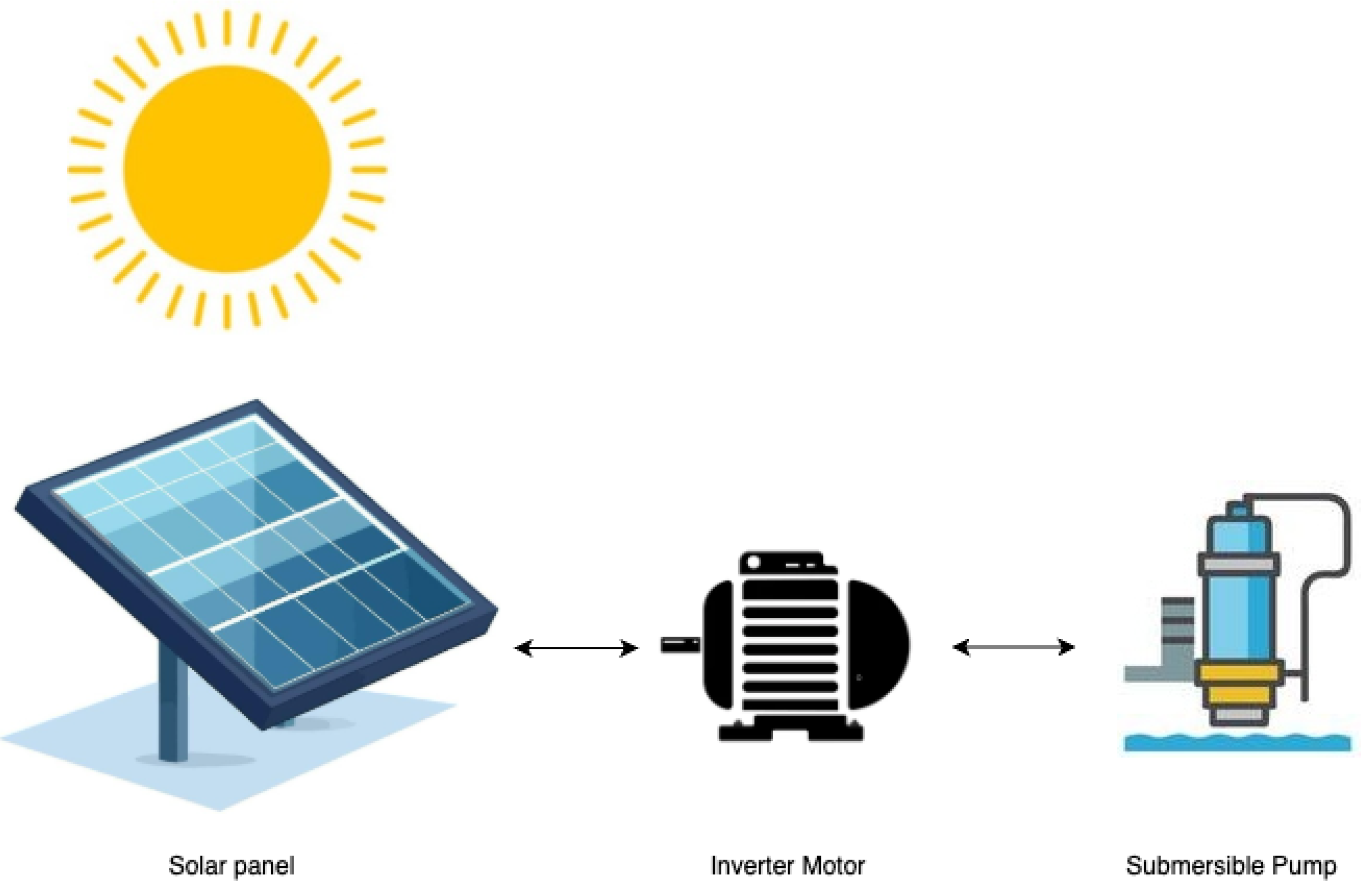
Figure 1. System Design.
Inventions 10 00093 g001
Figure 2. AI-Based Predictive Model Process Flow.
Inventions 10 00093 g002
Figure 3. Total dynamic head (TDH) [54].
Inventions 10 00093 g003
Figure 4. Comparative Model Metrics Across Training, Validation, and Testing Sets (Output Frequency Prediction).
Inventions 10 00093 g004
Figure 5. Actual vs. Predicted Values for All Models on the Test Set (Output Frequency Prediction).
Inventions 10 00093 g005
Figure 6. Absolute Error Percentiles Comparison (Test Set-Hz).
Inventions 10 00093 g006
Figure 7. Feature Importance and Coefficients for All Models (Output Frequency Prediction).
Inventions 10 00093 g007
Figure 8. Comprehensive Feature-Feature Correlation Matrices: Pearson, Spearman, and Kendall.
Inventions 10 00093 g008
Figure 9. Comparative Model Metrics Across Training, Validation, and Testing Sets (Output Power Prediction).
Inventions 10 00093 g009
Figure 10. Actual vs. Predicted Values for All Models on the Test Set (Output Power Prediction).
Inventions 10 00093 g010
Figure 11. Absolute Error Percentiles Comparison (Test Set-kW).
Inventions 10 00093 g011
Figure 12. Water Distribution of Water Volume Lifted from Reservoir on Monthly Basis.
Inventions 10 00093 g012
Table 1. PV Panel Specifications.
PV Panel ModelSuntech STP340-A72/Vfh
Rated power340 W
Rated voltage37.9 V
Rated current8.98 A
Open circuit voltage46.0 V
Short circuit current9.5 A
Module efficiency17%
Total number of PV panels96 panels
Connection6 strings, each string consists of 16 series PV panels
Table 2. Inverter Specifications.
Inverter ModelYASKAWA AC Drive GA700
Rated power(30 Hp/22 Kw)
Rated output current45 A
Rated voltage3 phases/380 V
Control methodV/F
Table 3. Pump Specifications.
Pump ModelVansan VSPss04090/6.B2
Rated power30 Hp
Stages6
MaterialStainless steel
Outlet connection diameter4 inches
Table 4. Motor Specifications.
Motor ModelVansan VSMOF4/30T
Rated power30 Hp
Rated voltage3 phases/380 V
ShaftStainless steel
Outlet connection diameter4 inches
Table 5. Optimized Hyperparameters for Tree-Based Models (Phase 1).
HyperparameterRandom ForestGradient BoostingXGBoost
Number of Estimators300500500
Maximum Depth344
Minimum Samples Split54
Minimum Samples Leaf22
Learning Rate0.030.03
Subsample Ratio0.90.9
Maximum Features0.8
Column Subsample Ratio by Tree0.8
Gamma0.1
Table 6. Final Optimized Hyperparameters for Neural Network 1 (NN1).
HyperparameterValue
Learning Rate0.005
Batch Size128
Epochs (Max)150
Number of Hidden Layers2
Neurons per Layer64
Dropout Rate0.2
Activation FunctionReLU
Table 7. Optimized Hyperparameters for Tree-Based Models (Phase 2).
HyperparameterRandom ForestGradient BoostingXGBoost
Number of Estimators200300300
Learning Rate0.020.050.05
Maximum Depth244
Minimum Samples Split44
Minimum Samples Leaf22
Subsample Ratio0.80.8
Maximum Featuressqrt
Column Subsample by Tree0.8
Gamma0.1
Table 8. Optimized Hyperparameters for Neural Network 2 (NN2).
HyperparameterValue
Learning Rate0.001
Batch Size32
Epochs (Max)100
Early Stopping Patience10
Number of Hidden Layers2
Neurons per Layer[64, 32]
Dropout Rate0.2
Activation FunctionReLU
Table 9. Training Metrics for All Models in Predicting Output Frequency (Phase 1).
ModelTrain R2Train MSETrain RMSETrain MAE
Persistence Baseline0.0001986.331.5323.18
Linear Regression0.922938.366.193.21
Random Forest0.98955.212.280.75
Gradient Boosting0.960719.564.421.83
XGBoost0.98368.192.861.07
Neural Network0.956821.534.641.89
Table 10. Validation Metrics for All Models in Predicting Output Frequency (Phase 1).
ModelVal R2Val MSEVal RMSEVal MAE
Persistence Baseline0.0001986.331.5323.18
Linear Regression0.923238.396.203.23
Random Forest0.978810.593.250.99
Gradient Boosting0.958420.824.561.85
XGBoost0.976211.923.451.21
Neural Network0.955022.504.741.89
Table 11. Test Metrics with R-squared and MSE for All Models (Phase 1).
ModelTest R2Test MSE
Persistence Baseline0.0001986.3
Linear Regression0.921339.27
Random Forest0.978410.77
Gradient Boosting0.959220.36
XGBoost0.977011.47
Neural Network0.954922.51
Table 12. Test RMSE with Variability for All Models (Phase 1).
ModelTest RMSE
Persistence Baseline31.53
Linear Regression6.27 (Std Dev: 0.14, 95% CI: [5.98, 6.55])
Random Forest3.28 (Std Dev: 0.13, 95% CI: [3.04, 3.53])
Gradient Boosting4.51 (Std Dev: 0.13, 95% CI: [4.25, 4.76])
XGBoost3.39 (Std Dev: 0.12, 95% CI: [3.15, 3.63])
Neural Network4.74 (Std Dev: 0.14, 95% CI: [4.47, 5.01])
Table 13. Test MAE with Variability for All Models (Phase 1).
ModelTest MAE
Persistence Baseline23.18 (Baseline)
Linear Regression3.24 (Std Dev: 0.05, 95% CI: [3.14, 3.34])
Random Forest1.00 (Std Dev: 0.03, 95% CI: [0.95, 1.06])
Gradient Boosting1.85 (Std Dev: 0.04, 95% CI: [1.77, 1.93])
XGBoost1.20 (Std Dev: 0.03, 95% CI: [1.14, 1.27])
Neural Network1.91 (Std Dev: 0.04, 95% CI: [1.82, 2.00])
Table 14. Phase 1 Test RMSE with Wilcoxon Signed-Rank Significance (Part 1).
ModelTest RMSE95% CIvs. Linear Regressionvs. Random Forest
Linear Regression6.27[5.98, 6.55]-3.08 × 10−164
Random Forest3.28[3.04, 3.53]3.08 × 10−164-
Gradient Boosting4.51[4.25, 4.76]8.15 × 10−1631.05 × 10−122
Table 15. Phase 1 Test RMSE with Wilcoxon Signed-Rank Significance (Part 2).
ModelTest RMSEvs. Gradient Boostingvs. XGBoost
XGBoost3.393.33 × 10−165-
Neural Network4.74-3.33 × 10−165
Table 16. Training and Inference Times for Machine Learning Models (Phase 1).
ModelTrain Time (s)Test Inf. Time (s)Time/Sample (s)
Linear Regression0.01490.00130.000000
Random Forest14.36780.17750.000016
Gradient Boosting8.12790.01910.000002
XGBoost0.54250.02500.000002
Neural Network678.21150.68620.000062
Table 17. Comprehensive Correlation Analysis: Features vs. Output Frequency.
FeaturePearson (r)Spearman ( ρ )Kendall ( τ )
Frequency Reference0.9520.9630.874
uvIndex (W/m2)0.7400.7580.594
Humidity (%)−0.571−0.583−0.431
Air Temperature (°C)0.4370.4510.326
Wind Speed (m/s)0.4010.4090.294
Table 18. Variance Inflation Factor (VIF) for Input Features.
FeatureVIF
Humidity (%)3.04
Air Temperature (celsius)2.62
Frequency Reference2.16
uvIndex (W/m2)2.08
Wind Speed (m/s)1.23
Table 19. Maximum Feature-Feature Correlations and Redundancy Threshold Assessment.
MetricFeature PairCorrelationExceeds 0.80?
PearsonuvIndex ↔ Air Temperature−0.780No
SpearmanuvIndex ↔ Air Temperature−0.821Yes
KendalluvIndex ↔ Air Temperature−0.613No
Table 20. Training Metrics for All Models in Predicting Output Power (Phase 2).
ModelTrain R2Train MSETrain RMSETrain MAE
Persistence Baseline−0.0195.009.759.20
Linear Regression0.000389.769.478.97
Random Forest0.93216.102.471.21
Gradient Boosting0.107980.108.958.39
XGBoost0.129178.208.848.03
Neural Network0.004489.399.458.94
Table 21. Validation Metrics for All Models in Predicting Output Power (Phase 2).
ModelVal R2Val MSEVal RMSEVal MAE
Persistence Baseline−0.0195.009.759.20
Linear Regression0.000189.929.488.98
Random Forest0.88969.933.151.46
Gradient Boosting0.105380.468.978.41
XGBoost0.124278.768.878.05
Neural Network0.005289.479.468.94
Table 22. Test Metrics with R-squared and MSE (Phase 2).
ModelTest R2Test MSE
Persistence Baseline0.000088.50
Linear Regression0.000788.50
Random Forest0.90078.89
Gradient Boosting0.110278.20
XGBoost0.137877.10
Neural Network0.005188.90
Table 23. Test RMSE with Variability (Phase 2).
ModelTest RMSE95% CI/Std Dev
Persistence Baseline9.41[9.37, 9.45] (0.02)
Linear Regression9.46[9.42, 9.50] (0.021)
Random Forest2.98[2.87, 3.09] (0.054)
Gradient Boosting8.92[8.88, 8.97] (0.023)
XGBoost8.79[8.72, 8.85] (0.032)
Neural Network9.44[9.40, 9.48] (0.021)
Table 24. Test MAE with Variability (Phase 2).
ModelTest MAE95% CI/Std Dev
Persistence Baseline8.91[8.86, 9.00] (0.028)
Linear Regression8.94[8.89, 9.00] (0.029)
Random Forest1.39[1.35, 1.44] (0.024)
Gradient Boosting8.36[8.31, 8.42] (0.029)
XGBoost7.97[7.90, 8.03] (0.034)
Neural Network8.92[8.86, 8.97] (0.029)
Table 25. Phase 2 Test RMSE with Wilcoxon Signed-Rank Significance (Part 1).
ModelTest RMSE95% CIvs. Linear Regressionvs. Random Forest
Linear Regression9.46[9.42, 9.50]-1.02 × 10−150
Random Forest2.98[2.87, 3.09]1.02 × 10−150-
Gradient Boosting8.92[8.88, 8.97]5.44 × 10−1453.21 × 10−130
Table 26. Phase 2 Test RMSE with Wilcoxon Signed-Rank Significance (Part 2).
ModelTest RMSEvs. Gradient Boostingvs. XGBoost
XGBoost8.793.21 × 10−130-
Neural Network9.44-2.12 × 10−128
Table 27. Training and Inference Times for Machine Learning Models (Phase 2).
ModelTrain Time (s)Test Inf. Time (s)Time/Sample (s)
Linear Regression0.05200.00140.000000
Random Forest27.24170.34860.000000
Gradient Boosting5.22210.01320.000000
XGBoost0.43870.02380.000000
Neural Network828.26350.69220.000100
Table 28. Monthly and Yearly Water Usage Summary for 2024 (in Cubic Meters).
MonthVolume (m3)
January 20249784.20
February 202411,752.69
March 202411,212.82
April 202416,455.45
May 202415,737.80
June 202416,928.75
July 202418,276.96
August 202415,111.29
September 202413,894.36
October 202412,219.22
November 202412,389.35
December 202412,369.88
Total (Annual)166,132.77
Disclaimer/Publisher’s Note: The statements, opinions and data contained in all publications are solely those of the individual author(s) and contributor(s) and not of MDPI and/or the editor(s). MDPI and/or the editor(s) disclaim responsibility for any injury to people or property resulting from any ideas, methods, instructions or products referred to in the content.