Abstract
Non-intrusive load monitoring (NILM) enables the disaggregation of appliance-level energy consumption from aggregate electrical signals, offering a scalable solution for improving efficiency. This study compared the performance of traditional NILM algorithms (Mean, CO, Hart85, FHMM) and deep neural network-based approaches (DAE, RNN, Seq2Point, Seq2Seq, WindowGRU) under various experimental conditions. Factors such as sampling rate, harmonic content, and the application of power filters were analyzed. A key aspect of the evaluation was the difference in testing conditions: while traditional algorithms were evaluated under multiple experimental configurations, deep learning models, due to their extremely high computational cost, were analyzed exclusively under a specific configuration consisting of a 1-s sampling rate, with harmonic content present and without applying power filters. The results confirm that no universally superior algorithm exists, and performance varies depending on the type of appliance and signal conditions. Traditional algorithms are faster and more computationally efficient, making them more suitable for scenarios with limited resources or rapid response requirements. However, significantly more computationally expensive deep learning models showed higher average accuracy (MAE, RMSE, NDE) and event detection capability (F1-SCORE) in the specific configuration in which they were evaluated. These models excel in detailed signal reconstruction and handling harmonics without requiring filtering in this configuration. The selection of the optimal NILM algorithm for real-world applications must consider a balance between desired accuracy, load types, electrical signal characteristics, and crucially, the limitations of available computational resources.
1. Introduction
The global energy transition urgently requires innovative solutions to address the dual challenges of climate change mitigation. Households account for approximately 20–30% of global energy use [1], with inefficient monitoring systems exacerbating financial burdens and greenhouse gas emissions from fossil fuel dependence. Non-intrusive load monitoring (NILM) [2] has emerged as a transformative approach to enable granular energy management by disaggregating appliance-level consumption from aggregated electrical signals. While traditional methods rely on intrusive submetering, which is costly and impractical for large-scale deployment, NILM offers a scalable alternative. Yet, its widespread adoption remains hindered by unresolved technical limitations.
Since Hart’s seminal work in the 1980s [3], NILM algorithms [4,5] have evolved considerably, incorporating machine learning and advanced signal processing techniques. In recent years, research in NILM has progressed significantly with the application of deep learning architectures and innovative models that enhance the extraction of temporal patterns and complex features from electrical signals. For instance, a convolutional neural network (CNN)-based approach that leverages temporal patternization to capture more detailed usage patterns and improve appliance classification from power signals has been proposed, demonstrating notable improvements in both accuracy and robustness compared to traditional methods [6]. Similarly, a transformer-based model that employs attention mechanisms to extract global dependencies between the aggregate signal and individual device signals (overcoming the limitations of recurrent models and reducing data preprocessing requirements) was introduced in [7]. Furthermore, harmonic and generative modeling for NILM have been explored, showing that the explicit incorporation of harmonic information and generative techniques can enhance disaggregation performance, particularly in scenarios with high harmonic distortion [8].
However, critical barriers persist in inconsistent benchmarking due to heterogeneous datasets, sensitivity to sampling rates (varying from milliseconds to minutes), and inadequate handling of harmonic distortions or low-power noise. Current evaluations often overlook the interplay between algorithmic robustness and real-world variables, such as the electrical characteristics of appliances or computational constraints for real-time applications. This gap limits the practical implementation of NILM systems (see Figure 1), despite their proven potential to reduce household consumption by up to 20% through behavioral feedback.

Figure 1.
Advancing NILM for energy efficiency.
This paper advances NILM research by tackling key gaps in standardization, algorithmic evaluation, and metric-driven assessment. It promotes standardization using open-source tools, such as evaluating classical algorithms and neural network-based methods across diverse sampling rates, harmonic conditions, and power filters. The analysis integrates performance metrics, event detection, and computational efficiency to guide real-world deployment. By linking algorithmic performance [9] to dataset characteristics and hardware constraints, this work provides a framework for tailoring NILM solutions to specific appliance profiles and operational requirements [10]. The open tools and datasets underpinning this analysis enhance transparency, inviting replication and extension in future research.
2. Materials and Methods
Evaluating the performance of energy disaggregation algorithms requires a robust infrastructure for accurate data acquisition and standardized tools for comparative analysis. This study leverages datasets collected using open-source metering hardware, processed and analyzed through a dedicated software toolkit, and evaluated using a defined set of performance metrics under various experimental conditions.
2.1. Measurement Hardware
The datasets used in this study were generated using the OpenZmeter (oZm) platform, an open-source energy meter and power quality analyzer. While previous works describe versions v1 and v2 of the oZm, the core datasets analyzed in this article were obtained using the updated and high-precision oZm v3 [11]. This meter is distinguished by its capability to perform high-frequency electrical measurements at a sampling rate of 15,625 Hz, recording a broad spectrum of electrical variables, including voltage, current, and harmonics up to the 50th order for voltage, current, and power.
The oZm has been utilized in other research papers for different purposes, and its use in this work demonstrates the device’s robustness and versatility, establishing a new benchmark in high-frequency electrical monitoring for NILM research. Long-term data acquisition was facilitated via the oZm API.
2.2. Datasets
Evaluating the performance of energy disaggregation algorithms requires reliable electrical datasets that capture consumption at the aggregate and individual levels. In the field of NILM, the evaluation of algorithmic performance is fundamentally based on using such datasets. However, the heterogeneity of existing datasets often leads to inconsistency in algorithm benchmarking. Research on NILM has used several prominent public datasets for evaluation (see Figure 2), including the following:
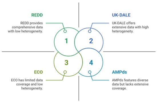
Figure 2.
NILM dataset characteristics.
- Reference Energy Disaggregation Dataset (REDD) [12], a public dataset used for energy disaggregation research.
- Minutely Power Dataset Almanac (AMPds) [13], a public dataset for load disaggregation and eco-feedback that includes data on the electricity, water, and natural gas consumption of residential households in Canada from 2012 to 2014.
- UK Domestic Appliance-Level Electricity (UK-DALE) dataset [14], obtained from a two-year longitudinal study of UK households [15].
- Electricity Consumption and Occupancy (ECO) dataset [16], which is used to evaluate the performance of NILM algorithms.
- Green Energy Consumption Dataset (GREEND) [17], which comprises data on household energy consumption in Italy and Austria.
This paper employed two publicly available datasets based on open hardware to address some of the challenges related to data variability and allow a focused analysis of the impact of sampling and filtering conditions. Both datasets were collected at the University of Almeria (Spain) using the oZm platform.
The first dataset was DSUALM10H [18], introduced in June 2023. This is a new high-resolution dataset for NILM and a multichannel dataset containing measurements of 10 common household appliances. It is distinguished by its ability to perform high-frequency electrical measurements at a sampling rate of 15,625 Hz. It captures a broad spectrum of electrical variables, including voltage, current, and harmonics up to the 50th order for voltage, current, and power. It includes 150 electrical variables, such as current, voltage, and power transients.
DSUALM10H was generated using three oZm v3, providing 12 measurement channels, 1 for aggregate consumption and 10 for individual appliances. The monitored appliances included an electric oven, a microwave, a kettle, a vacuum cleaner, a radiator, a television, an electric shower heater, a fan, a refrigerator, and a freezer. A feature of DSUALM10H is that it includes harmonic content for each appliance.
The second dataset was DSUALM10, which was derived from DSUALM10H. It was obtained by eliminating the harmonic components of voltage, current, and power, thus containing only the fundamental electrical measurements. Like DSUALM10H, it is based on measurements from the 10 appliances using the oZm v3. Both datasets are publicly available [18,19] and generated with open hardware, which promotes transparency and reproducibility in NILM research. They serve as a basis for exploring how signal characteristics and sampling conditions impact the performance of algorithms.
2.3. Software Tools and Evaluation Metrics
Energy disaggregation and algorithm evaluation were conducted using the Non-Intrusive Load Monitoring Toolkit (NILMTK) v0.4.0 [20], an open-source framework designed to streamline NILM research by providing standardized workflows, algorithms, data converters, and a suite of built-in evaluation metrics. Within this framework, custom converters were developed to process data. The evaluation methodology followed the full NILMTK pipeline (from raw data conversion to disaggregation assessment).
To extend its capabilities, the NILMTK-Contrib extension was employed [21], providing implementations of traditional algorithms and deep learning-based approaches. In addition, it offers a rapid experimentation API for cross-building and cross-dataset validation, as well as support for training on synthetic aggregates and transfer learning across different sampling frequencies [22].
Core NILMTK-supported metrics were used to evaluate algorithm performance, covering both power estimation (regression) and event detection (classification) aspects [23] as follows:
- 1.
- Mean Absolute Error (MAE) (Equation (1)), which measures the average absolute difference between the predicted and actual power consumption of an appliance. Lower MAE values indicate better estimation performance,where, predictedi and actuali represent the individual prediction values and actual energy consumption values of the appliances, respectively, and N represents the total number of observations.
- 2.
- Root Mean Squared Error (RMSE) (Equation (2)), which is like MAE, but gives greater weight to larger errors, represents the standard deviation of estimation errors,where represents the estimated power of device n at each time interval t, denotes the actual power of the same device, and T is the total number of observations or time intervals recorded during energy consumption.
- 3.
- F1-SCORE, which combines Precision (Equation (3)) and Recall (Equation (4)), assesses the accuracy in detecting ON/OFF events. A higher F1-SCORE reflects a better ability to correctly identify appliance operation states:TP represents true positives, FP false positives, and FN false negatives.
The F1-SCORE synthesizes these aspects, offering a composite measure that signals robust accuracy in identifying and predicting appliance states, as expressed in Equation (5):
- 4.
- Normalized Disaggregation Error (NDE), which quantifies the total energy estimation error for each appliance, is normalized by actual consumption to enable fair comparisons,where is the estimated power consumption of the device i at time t, and reflects the actual power consumption of the device over the total time interval T.
2.4. Algorithms
This study evaluated traditional algorithms and deep neural network-based models [24] for NILM using NILMTK and NILMTK-Contrib [24]. The main characteristics of the traditional algorithms are described below:
- Combinatorial Optimization (CO). This algorithm performs an exhaustive search of all possible combinations of appliance states to find the one that best explains the aggregate signal. While it can yield good results in simple scenarios, its complexity grows exponentially with the number of devices and possible states, which limits its scalability [25].
- Hart85. Based on finite state machines, this method detects ON/OFF events using dynamic active/reactive power thresholds. It is susceptible to parameter configuration and signal quality, showing highly variable performance depending on the appliance type and experimental conditions [3].
- Mean. This method uses a moving average of the aggregate consumption signal over a time window to estimate the consumption of each appliance. It is notable for its simplicity, robustness, and low computational demand, although its accuracy may be limited for devices with complex or variable consumption patterns.
- Factorial Hidden Markov Model (FHMM) [26]. This probabilistic model uses the Viterbi algorithm to infer the most probable sequence of device states, considering temporal transitions and relationships between them, with complexity O(T·SN) [27]. Unlike the standard FHMM implementation in NILMTK, this version incorporates several optimizations to improve efficiency; it leverages parallel processing on multicore CPUs via multithreading, replaces Python 3.7.12 loops with vectorized NumPy operations, manages the state space more efficiently through probability precomputing and dynamic pruning, optimizes memory usage with adjustable data types and sparse array storage, and uses JIT compilation with Numba for critical routines. In contrast, the original NILMTK version relies on sequential, generic implementations and non-vectorized data structures, resulting in substantially lower computational performance and resource efficiency.
The main characteristics of deep neural network-based models are as follows:
- WindowGRU. Implemented as a bidirectional GRU network that processes temporary windows of aggregate electrical consumption, WindowGRU uses recurring layers with ReLU activation to predict the state of appliances in the last temporal step, is integrated into the NILMTK experimentation API for cross-evaluation between datasets, and is typically trained with Adam (30 epochs, learning rate 1 × 10⁻³) under GPU requirements (TensorFlow-GPU + CUDA) and normalization preprocessing, although non-optimized implementations of the activation functions may limit its practical performance [21].
- Seq2Seq. This model implements an encoder–decoder-based deep neural network architecture, where a time window of the aggregated signal (e.g., 99 samples) is processed by the model to predict the corresponding sequence of consumption of an appliance, using recurrent and convolutional layers; each device has its own trained model, training is performed with normalized and batch data, and integration with the NILMTK API allows performance to be evaluated in different buildings and datasets in a flexible and reproducible way [21,28].
- Denoising Autoencoder (DAE). Fully convolutional in this implementation, it uses Conv1D layers in the encoder (e.g., 3 layers with 8/16/32 filters and kernel = 4) and a symmetric transposed decoder to capture temporal patterns, injecting Gaussian noise (σ = 0.1–0.3) into the aggregate input to strengthen the model, and optimizes a combined loss function that integrates the Mean Square Error (MSE) of reconstruction with L1 regularization over the weights (controlled by λ) to avoid overfitting. Training is with Adam (learning rate ~1 × 10⁻³) on time windows of 150–600 standardized samples, thus achieving disaggregation through sparsa and locally invariant latent representations [21].
- Recurrent Neural Networks (RNN). This model implements standard recurrent neural networks for energy disaggregation, processing temporal sequences of aggregate consumption through predefined windows (e.g., 100–600 samples). Each appliance has an independent RNN model trained with recurrent dense layers and ReLU activation, using Keras as a backend. The data are normalized and screened before training, which is performed with the Adam optimizer (learning rate ~1 × 10⁻³) and MSE loss function, integrated into the NILMTK API for cross-evaluation between buildings/datasets. The current implementation faces practical limitations due to version-specific dependencies (TensorFlow/Keras) and problems reported in the train–test division after migrating to internal Keras methods [21].
- Seq2Point. This model implements a CNN-based neural network that takes temporal windows of the aggregated signal (e.g., 99 samples) and predicts the consumption value of an appliance only at the center point of the window, using a sequential architecture of Conv1D, Dense, Dropout, and Flatten layers, trained with MSE loss function, data normalization, and hyperparameter configuration, such as window size, epoch number, and batch size, all integrated into NILMTK’s rapid experimentation API to facilitate training, evaluation, and comparison between devices and datasets [29].
2.5. Experimental Conditions
To explore how different factors influence algorithm performance, evaluations were conducted under multiple experimental conditions, focusing on the following:
- Sampling rate. Tested at intervals ranging from 90 and 60 s to higher resolutions (1 s, 500 ms, 250 ms, and 125 ms).
- Harmonic content. By comparing DSUALM10H (with harmonics) and DSUALM10 (without them), the impact of harmonic components was assessed [18].
- Power filtering. The effect of applying aggregate power thresholds (10 W, 50 W, 100 W) was evaluated before disaggregation.
This multifactorial evaluation (employing DSUALM10, DSUALM10H, and NILMTK metrics) aimed to comprehensively understand energy disaggregation algorithms’ behavior.
3. Results and Discussion
This section presents the evaluation outcomes for various energy disaggregation algorithms applied to DSUALM10H and DSUALM10, using the NILMTK-Contrib tool. In addition, the influence of different experimental conditions was investigated, including the application of power filters, the type of appliance, the sampling rate, and the presence of harmonics. Regarding algorithm performance, the results of visual disaggregation and an analysis of the execution times for all the algorithms considered are also included.
3.1. Evaluation Metrics
Four key metrics (MAE, NDE, F1-SCORE, and RMSE) were used to evaluate algorithm performance under identical experimental conditions (sampling rate, harmonic presence, power filters) for household appliances, with an 80/20 train–test data split, ensuring consistent scenario comparisons across metrics [22]. The inability to use sub-second sampling intervals for deep learning algorithms in NILMTK-Contrib (e.g., CNNs, LSTMs), unlike classical methods (CO, FHMM), stems from architectural constraints: classical approaches rely on statistical/discrete-event models independent of temporal granularity, while neural networks require fixed-length input windows (e.g., 500 samples at 1 s = 500 s context), where shorter intervals (<1 s) reduce effective temporal context, eroding long-term pattern capture, which is critical for performance. Additionally, higher sampling frequencies exponentially increase data volume and computational demands, and current NILMTK-Contrib implementations lack mechanisms to adapt hyperparameters (e.g., kernel sizes, pooling layers) to sub-second scales, unlike signal-level filters applicable across frequencies. The detailed results of the MAE, NDE, F1-SCORE, and RMSE metrics for all algorithms and experimental conditions are presented in Appendix A.
3.1.1. F1-SCORE
Figure 3 shows that, in general, neural network-based algorithms achieve higher or comparable F1-SCOREs to traditional algorithms for most home appliances. This suggests that neural networks are more robust and effective at handling the complexity and variability of electrical signals, especially in the presence of harmonics and unfiltered. However, there are exceptions: for example, the traditional Mean algorithm obtains an exceptionally high F1-SCORE for the TV, and Hart85 achieves good results only for some appliances.
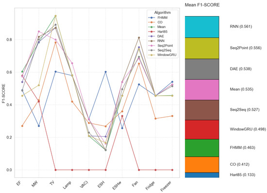
Figure 3.
F1-SCORE per algorithm and appliance (electric furnace (EF), microwave (MW), television (TV), incandescent lamp (Lamp), vacuum cleaner (VAC), electric space heater (ESH), electric shower heater (ESHw), fan, fridge, and freezer.).
On the other hand, while neural networks often outperform traditional algorithms, they also present difficulties in specific applications, such as vacuum cleaners and electric space heaters, where F1-SCOREs are low even for these advanced models. This indicates that, despite their sophistication, neural networks cannot always correctly detect all events in appliances with more complex or less predictable consumption patterns. In summary, the analysis confirms that, under the condition of 1-s sampling with harmonic content, neural networks offer a better capacity for event detection than traditional algorithms, showing a more balanced and robust performance against different types of appliances. Nevertheless, this advantage is accompanied by a considerably higher computational cost, which can limit practical applications.
3.1.2. MAE
The MAE varies considerably for traditional algorithms depending on the algorithm, appliance, and conditions. Stable and straightforward appliances such as the TV or fan have lower MAEs, especially with Mean. High-power or complex appliances, such as the electric oven, consistently present high MAEs with all traditional algorithms. Hart85 significantly improves its MAE by applying power filters.
Neural network-based algorithms, evaluated in the configuration of 1 s with harmonic content, generally outperform classical algorithms in all average metrics, including MAE. They tend to achieve lower MAEs, even for complex or high-powered appliances. For example, for the electric furnace, the MAE of RNN was 174.46 W, while Seq2Point was 285.67 W, Seq2Seq was 389.78 W, and DAE was 480.55 W. These values are considerably lower than the MAE reported for Mean (910.21 W), CO (553.7 W), and FHMM (322.3 W) without filters, and in some cases, even better than Hart85 (423.29 W) without filters. This reinforces the idea that neural models can better model complex consumption patterns. Figure 4 shows the differences in MAE per appliance among all the algorithms evaluated (including DAE, RNN, Seq2Point, Seq2Seq, and WindowGRU).
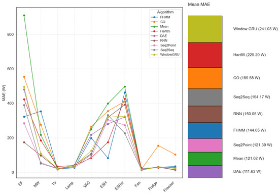
Figure 4.
MAE per algorithm and appliance (electric furnace (EF), microwave (MW), television (TV), incandescent lamp (Lamp), vacuum cleaner (VAC), electric space heater (ESH), electric shower heater (ESHw), fan, fridge, and freezer.).
3.1.3. NDE
In traditional algorithms, Mean performs better with low NDEs for regular, unfiltered, low-consumption appliances. At the same time, Hart85 presents poor performance under these conditions, improving with the application of filters (see Figure 5).
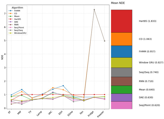
Figure 5.
NDE per algorithm and appliance (electric furnace (EF), microwave (MW), television (TV), incandescent lamp (Lamp), vacuum cleaner (VAC), electric space heater (ESH), electric shower heater (ESHw), fan, fridge, and freezer.).
The fridge has the worst overall performance with traditional algorithms. Algorithms based on neural networks, under the conditions evaluated (1 s with harmonic content), also present generally lower NDE on average than traditional algorithms, reflecting a greater precision in estimating normalized energy consumption. For the electric oven, the NDEs of RNN (0.295), Seq2Point (0.438), Seq2Seq (0.500), and DAE (0.610) are substantially lower than those of traditional unfiltered algorithms, indicating a better ability to estimate the consumption of this high-power appliance. For the fridge, whose NDEs are high with some traditional algorithms, the neural networks obtained NDEs between 0.762 and 0.7945, representing an improvement. The NDE confirms that while Mean is effective for regular loads, neural networks offer more robust performance for various consumption patterns.
3.1.4. RMSE
Like MAE, Mean shows the lowest RMSEs for stable, low-power unfiltered appliances (see Figure 6). Hart85 has a significantly high RMSE without filters, but improves substantially with its application. The electric oven consistently presents the highest RMSEs among all traditional appliances and algorithms. CO shows a significant increase in RMSE for the fridge and freezer with filters.
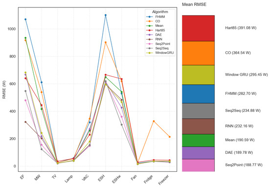
Figure 6.
RMSE per algorithm and appliance (electric furnace (EF), microwave (MW), television (TV), incandescent lamp (Lamp), vacuum cleaner (VAC), electric space heater (ESH), electric shower heater (ESHw), fan, fridge, and freezer.).
By including the neural network algorithms evaluated in the condition of 1 s with harmonic content, it is observed that they generally achieve lower RMSEs on average than classical algorithms. This is particularly notable for high-powered appliances such as the electric oven, where the RMSEs of RNN (323.0 W), Seq2Point (479.9 W), Seq2Seq (547.8 W), and DAE (667.6 W) are lower than those of traditional unfiltered algorithms, indicating a better ability to handle significant power fluctuations. Although Hart85 can achieve low RMSEs for high-power loads with filters, neural networks accomplish this without relying on this specific preprocessing in the tested configuration. The RMSE analyses, such as the MAE and NDE, underline that neural networks offer greater overall accuracy in estimating power, even in the presence of harmonics, although at a considerably higher computational cost.
The inclusion of algorithms based on neural networks in the analysis of metrics such as F1-SCORE, MAE, NDE, and RMSE allows a more complete evaluation, since these models usually outperform traditional algorithms on average and demonstrate a greater ability to handle the complexity and variability of appliances, especially without the need for filters; however, this better performance implies a much higher computational cost, so the choice of the most appropriate algorithm must balance the desired accuracy, the characteristics of the devices to be monitored, and the resource limitations of the environment where it will be implemented.
3.2. Influence of Experimental Factors
The following section discusses the impact of specific experimental conditions (filters, appliance type, sampling rate) on evaluation metrics.
3.2.1. Effect of Power Filtering
The comparative analysis of the influence of power filters on the disaggregation of electricity consumption metrics shows that, when evaluating the average of all appliances, the classical algorithms experience a slight improvement in absolute errors (MAE, RMSE) when applying a power filter (e.g., 100 W). However, this improvement is marginal and is accompanied by a degradation in the ability to detect events, especially in small and cyclic loads, as evidenced by the drop in the average F1-SCORE in the Hart85 algorithm. In contrast, the Mean algorithm demonstrates greater robustness, maintaining stable performance across all metrics despite filtering. Nonetheless, the improvements remained relatively limited (see Figure 7).
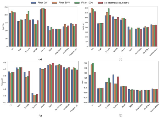
Figure 7.
Metrics, including harmonics and filters. (a) MAE, (b) RMSE, (c) F1-SCORE, (d) NDE.
The results show that combining harmonics with deep learning techniques such as Seq2Point and RNN, along with low filter values, optimizes the F1-SCORE in the experimental framework analyzed. In contrast, the use of high filter values improves the RMSE in RNN, and the inclusion of harmonics benefits the performance of Seq2Seq, although it is detrimental to FHMM. Neural networks, specifically RNN and Seq2Point, exhibit up to 54% less error compared to traditional methods such as FHMM. To minimize NDE, neural networks—particularly Seq2Point and Seq2Seq—with medium to high filter values (50–100 W) and the use of harmonics, are the most efficient option, which contrasts with the results observed for F1-SCORE, where the Mean method stands out. Finally, to reduce MAE, neural networks, especially RNN with a filter value of 50 W and Seq2Point, prove to be optimal, while statistical methods such as Mean show significant limitations in numerical accuracy. This analysis highlights the superiority of neural architectures over conventional statistical approaches, both in terms of accuracy and adaptability to different evaluation metrics.
Neural network-based algorithms, evaluated with and without filtering despite their computational demands, demonstrate clear superiority over traditional methods across all average metrics, achieving superior MAE, RMSE, F1-SCORE, and NDE values. This indicates greater accuracy in estimating the energy consumed and detecting events in all appliances, not just high-power ones. Although neural models require more computational resources, their overall performance is superior, and they do not depend on filtering to obtain good results.
The figure summarizes these findings, highlighting that filtering only partially benefits classical algorithms and can distort the overall evaluation by impairing the detection of minor loads. At the same time, neural networks offer more balanced and accurate performance across the complete set of devices.
3.2.2. Effect of Type of Application
The performance of the algorithms used for energy disaggregation depends mainly on the type of appliance analyzed. In the case of appliances with stable and straightforward consumption patterns, such as televisions, fans, or incandescent lamps, classical algorithms, especially the Mean method, usually offer the best results in terms of accuracy and stability, showing excellent robustness to variations in the electrical signal. However, in high-powered devices or devices with more complex consumption patterns, such as electric ovens, heaters, or vacuum cleaners, errors in metrics increase for all algorithms. In these cases, models based on deep neural networks achieve better results in error metrics and event detection, outperforming classical methods, especially when power filters are not applied (see Figure 8a–d).

Figure 8.
Heat map for appliances and algorithms. (a) F1-SCORE, (b) RMSE, (c) NDE, (d) MAE.
Traditional algorithms exhibit reduced performance for appliances that exhibit cyclical or intermittent patterns, such as refrigerators, freezers, or microwaves, especially if filters are applied. Neural models maintain competitive values and can better model these complex patterns. In general, no algorithm is superior in all cases: the Mean method is efficient for simple loads but loses competitiveness in more complicated scenarios. Algorithms such as Hart85 can improve in specific contexts. However, their performance is inconsistent, while neural methods offer a more balanced and robust performance against a greater variety of consumption patterns (but with more computational resources).
The choice of the most appropriate algorithm for energy disaggregation must consider both the type of appliance and the particularities of its consumption. Classical methods are recommended for stable and straightforward loads. At the same time, neural models are more appropriate for devices with complex consumption, high power, or cyclic patterns, provided that the necessary computational capacity is available.
3.2.3. Effect of the Sampling Rate
Sampling frequency is a key factor in energy disaggregation, as it determines the ability of algorithms to detect rapid events and complex patterns in appliance consumption. In classical algorithms, a higher sampling rate (1 s) significantly improves error metrics (MAE, RMSE, NDE) and event detection capability (F1-SCORE). As the interval between samples increases, errors increase and the F1-SCORE decreases, as brief events and rapid changes in consumption are lost, especially at small or intermittent loads. For example, the average MAE of the Mean algorithm drops from about 400 to 280 W, and the F1-SCORE improves from 0.48 to 0.51, when the sample rate increases from 90 s to 1 s, reflecting the importance of high-frequency measurement for accurate disaggregation (see Table 1). The higher the sampling frequency, the classical algorithms show fewer errors and higher F1-SCORE, especially in the Mean and CO algorithms, while decreasing the frequency (60 s or 90 s) results in increased errors and a decreased F1-SCORE; Hart85 and FHMM are less sensitive in F1-SCORE but their errors also grow less frequently, with Mean standing out as the most robust and stable algorithm.

Table 1.
Metric averages based on sample rate, unfiltered, and with harmonic content.
In the case of algorithms based on deep neural networks, this study only evaluates the 1 s sampling condition due to its high computational cost. Although there is no direct data on the impact of reducing the frequency in these models, it is inferred that, as in the classical models, a lower frequency would degrade their performance by losing relevant temporal information. The neural models, evaluated at 1 s, present average metrics higher than the classical ones at any frequency, suggesting they make the most of the available temporal detail.
In summary, a high sampling rate is preferable to achieve maximum accuracy in energy disaggregation. However, it must be balanced with computational cost, especially in real-time or resource-constrained applications.
3.2.4. Effect of Harmonic Content
The presence of harmonics in the electrical signal variably affects the performance of energy disaggregation algorithms. In deep neural network-based models, the metrics were obtained with harmonics. Under these conditions, these algorithms show a robust and competitive performance, with an average F1-SCORE higher than most classical algorithms and errors generally lower for most appliances, especially in 1-s sampling setups and without a power filter. Therefore, harmonics do not prevent good results from detecting events and estimating power, surpassing the classics in most cases under the same conditions.
Classical algorithms were evaluated with and without harmonic content. Direct comparison of average metrics shows that the presence of harmonics does not produce drastic changes in the overall performance of these methods. However, it may cause slight variations in error metrics and event detection capability, depending on the type of appliance and experimental configuration. In general, Mean maintains its robustness and stability with or without harmonics, while Hart85, CO, and FHMM show small fluctuations in their metrics, but without a clear pattern of systematic deterioration. Harmonics can slightly affect the accuracy of event detection and slightly increase estimation errors in some devices. Still, the effect is usually less than that caused by other factors, such as the sampling rate or the application of filters.
In summary, the effect of the harmonic content on energy disaggregation metrics is limited compared to other experimental factors. Neural network-based algorithms maintain competitive performance even with harmonic content, and classical algorithms exhibit only slight variations in their metrics under these conditions. Therefore, the presence of harmonics does not represent a significant obstacle to the effectiveness of deep neural models in energy disaggregation tasks.
3.3. Disaggregated Data and Execution Times
The disparity in execution times between algorithms directly impacts their practical applicability. Traditional methods are considerably faster than deep learning-based approaches. Visual fidelity in reconstructing individual signals generally correlates with longer execution time. Traditional algorithms are distinguished by their computational efficiency, being generally much faster than neural networks. However, their performance and visual detail vary.
Mean is the fastest algorithm, with extremely low execution times (0.91 s for the visualization). It offers a considerably simplified disaggregation, as shown in Figure 9a. In terms of metrics, Mean is extremely efficient and accurate for stable and straightforward loads such as TVs or fans, showing low MAEs for these (e.g., TV 20.89, Fan 15.89, under 1 s, harmonics, no filter). However, its accuracy limits its usefulness for appliances with complex or high-power patterns, which usually have the highest MAE (e.g., 910.21 W in the electric oven). Despite this limitation, the Mean algorithm remains robust to variations, maintaining stable metrics even with filtering.
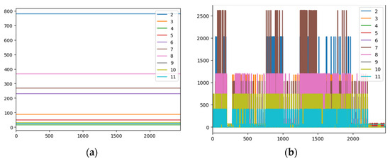
Figure 9.
Disaggregated data for DSUALM10H. (a) Using Mean, (b) using CO. (Appliances: electric furnace (2), microwave (3), television (4), incandescent lamp (5), vacuum cleaner (6), electric space heater (7), electric shower heater (8), fan (9), fridge (10), and freezer (11)).
The CO algorithm is fast and maintains low and stable execution times (2.39 s for visualization with harmonics). It offers a remarkable level of disaggregation detail for its low computational cost (Figure 9b), which is often higher than other traditional methods. However, its behavior can be more erratic, being sensitive to the sampling rate and filters, and it can deteriorate significantly for cyclical appliances such as the refrigerator or freezer The 1 s configuration with harmonic content, without a filter, features high MAEs for the fridge (155.15 W) and the freezer (103.80 W), which can align with the observation that harmonics have a negative effect.
The FHMM algorithm has a considerably longer execution time than Mean and CO (25.67 s). Despite the increased computational effort, the level of visual detail in the disaggregation shown is surprisingly modest compared to CO (Figure 10a). It is noticeably slower than Mean and CO, which limits its viability in rapid response scenarios. Regarding the MAE values in the 1 s configuration with harmonic content, without filter, the values range from relatively low values for appliances such as the TV (18.56 W) to substantially higher values for more complex devices, such as the electric oven (322.33 W).
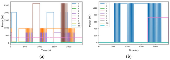
Figure 10.
Disaggregated data for DSUALM10H using FHMM (a) and Hart85 (b). The appliances are electric furnace (2), microwave (3), television (4), incandescent lamp (5), vacuum cleaner (6), electric space heater (7), electric shower heater (8), fan (9), fridge (10), and freezer (11).
Hart85 exhibits slower execution than Mean and CO but is still manageable for non-strict environments (Figure 10b). Without filters, the MAE tends to be high in several appliances, such as the TV, fan, refrigerator, and freezer (TV 33.72 W, fan 23.88 W, fridge 26.61 W, freezer 24.34 W). Its performance improved with the application of power filters. Its dependence on the sampling rate is extreme, with near-zero performance in event detection at high frequencies without filters.
Algorithms based on deep neural networks offer greater fidelity in reconstructing individual signals at the cost of much higher computational demand. They were evaluated without a filter due to their high cost and their metrics were obtained with harmonics in 1 s sampling. They outperform classical algorithms in all average metrics when evaluated without a filter and with harmonic content.
DAE has a considerable execution time for visualization (555.63 s) with a window size of 99. It offers a much richer level of disaggregation, identifying specific consumption patterns. The MAEs in the 1 s configuration with harmonic content (Figure 11a) are generally low (e.g., microwave 108.51 W, TV 19.61 W, fan 14.59 W).
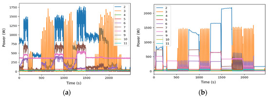
Figure 11.
Disaggregated data for DSUALM10H. (a) Using DAE, (b) using RNN. (Appliances: electric furnace (2), microwave (3), television (4), incandescent lamp (5), vacuum cleaner (6), electric space heater (7), electric shower heater (8), fan (9), fridge (10), and freezer (11).)
The scale of the Y-axis varies between algorithms because each NILMTK disaggregation method (such as Mean, CO, FHMM, or DNN) estimates appliance power from the total signal in a different way: simpler algorithms such as Mean tend to smooth the values and underestimate peaks, resulting in lower maximum power values. In contrast, others, such as CO, are more sensitive to abrupt changes and can estimate significantly higher maximum values. These differences reflect the unique behavior of each algorithm when interpreting and separating the power signal, so the variation in scale does not indicate an error, but rather the diversity in how each model processes and represents energy consumption.
RNN, while one of the most computationally expensive methods (11,892.43 s), offers a remarkable improvement in visual accuracy (Figure 11b). However, this benefit must be weighed against the high time cost, making it a suitable choice for applications where visual accuracy is a priority and computational resources are not a constraint.
Seq2Point has a runtime of 2012.42 s for visualization. The consistent disaggregated profile shows a good balance between complexity and detail (Figure 12a). The MAE is very low for several appliances (e.g., microwave 55.76, vacuum cleaner 87.95, electric shower heater 273.68 W, freezer 12.61 W). Seq2Seq completed the task in 857.34 s for visualization using a sequence length of 99, an epochs number of 10, and a batch size of 512. Their visual performance aligns with other neural models, evidencing good signal reconstruction, especially for complex loads (Figure 12b). It has the lowest MAE for the microwave (51.14 W) and the electric shower heater (226.71 W).
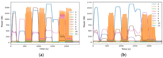
Figure 12.
Disaggregated data for DSUALM10H. (a) Using Seq2Point, (b) using Seq2Seq. (Appliances: electric furnace (2), microwave (3), television (4), incandescent lamp (5), vacuum cleaner (6), electric space heater (7), electric shower heater (8), fan (9), fridge (10), and freezer (11).)
WindowGRU is the algorithm that requires the longest processing time for visualization (16,283.86 s). Despite its high computational cost, the level of detail obtained is comparable to that of other deep learning models (Figure 13), suggesting that cost does not always translate into a commensurate improvement in quality. The MAEs are generally higher than other neural models for various appliances.
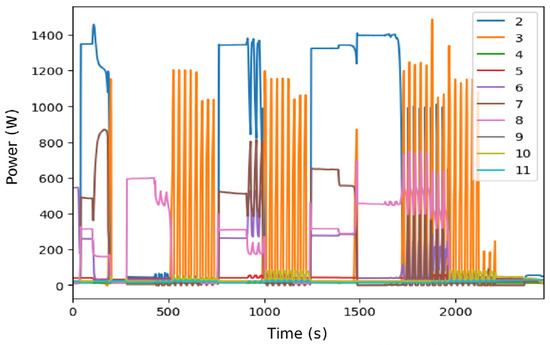
Figure 13.
Disaggregated data for DSUALM10H using WindowGRU. (Appliances: electric furnace (2), microwave (3), television (4), incandescent lamp (5), vacuum cleaner (6), electric space heater (7), electric shower heater (8), fan (9), fridge (10), and freezer (11).)
Although WindowGRU exhibits the longest execution, the level of disaggregation detail it produced was comparable to that of neural network-based algorithms, offering no clear advantage in output quality despite its significantly higher computational cost.
In summary, there is a clear correlation between the execution time and the level of visual detail of the disaggregation results. Traditional methods offer fast times, although with less precision. At the same time, algorithms based on neural networks provide greater fidelity in reconstructing individual signals at the cost of a greater demand on computational resources. This information is key when choosing an algorithm according to the constraints and objectives of the practical application.
Figure 14 illustrates the difference in logarithmic-scale execution times between traditional and deep learning methods of speed, multiplying by several orders of magnitude the Mean and CO times, which limits its viability in scenarios where response time is a critical factor.
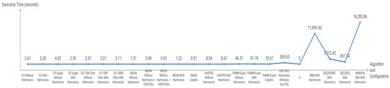
Figure 14.
Execution times by algorithm using a dedicated machine running Ubuntu 25.04, Intel Core i5-4210U CPU @ 1.70 GHz with 16 GB RAM and 500 GB SSD.
The analysis of average metrics (Figure 15) reveals a clear superiority of deep learning algorithms (Seq2Point, Seq2Seq, RNN, and DAE) over traditional methods, although with significant differences in execution times. Seq2Point stands out as the most balanced—with the best F1-SCORE (0.56), lowest MAE (111.63 W), and second-best RMSE (189.78 W)—but it requires 2012.42 s of processing. Seq2Seq achieves the best NDE (0.62) and RMSE (188.77 W) in 857.34 s, although with a slightly lower F1-SCORE (0.53). Traditional methods such as CO (1.22 s) and FHMM (66.31 s) show average performance (F1-SOCRE ≤ 0.464, MAE > 189 W), and Hart85 (8.67 s) presents a contradiction—good MAE/RMSE (144.05 W/282.7 W) but very poor F1-SCORE/NDE (0.114/0.957)—suggesting numerical accuracy at the expense of detection reliability. Mean shows limitations, with the worst MAE (241.03 W) despite an acceptable F1-SCORE (0.5) and minimal runtime (1.31 s), while WindowGRU (F1-SCORE = 0.5, MAE = 150.05 W) positions itself as an intermediate option but with the highest computational time (16,283.86 s). This hierarchy confirms that sequential models (Seq2Point/Seq2Seq) simultaneously optimize precision and consistency, but require up to 34 m of execution. In comparison, traditional methods excel in speed (≤1 m) at the cost of compromising key metrics, establishing a decisive trade-off between efficiency and performance.
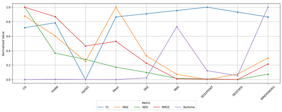
Figure 15.
Standardized comparison of NILMTK-Contrib algorithm metrics.
4. Conclusions
The systematic analysis of the performance of energy disaggregation algorithms under different experimental conditions, considering both execution times and quantitative metrics such as MAE, RMSE, F1-SCORE, and NDE, reveals that there is no universally superior algorithm. The performance of each approach intrinsically depends on the type of appliance, the experimental configuration (sampling rate, harmonic content, and application of power filters), and the characteristics of the model. Traditional algorithms, such as Mean, CO, Hart85, and FHMM, excel at computational efficiency and speed, making them particularly suitable for real-time applications or resource-constrained environments. Mean offers remarkable robustness against experimental variations and maintains low errors for simple loads, although its simplicity limits its accuracy with complex consumption patterns. CO and Hart85 have specific advantages, such as low run times and significant improvements through preprocessing. However, their performance may be affected by the cyclical nature of certain appliances or by sensitivity to the sample rate and filters applied.
On the other hand, algorithms based on deep neural networks (DAE, RNN, Seq2Point, Seq2Seq, WindowGRU) demonstrate a superior ability to reconstruct individual signals and achieve better average metrics in most scenarios, especially in harmonic-based and unfiltered configurations. These models excel at event detection and accurate power estimation and are better suited to the complexity and variability of modern appliances. However, its main limitation lies in the high computational cost, with execution times extending to several hours, which restricts its applicability in contexts where speed and efficiency are a priority.
The influence of experimental factors such as the sampling rate, the presence of harmonics, and the application of filters is also decisive, affecting each algorithm differently. While Mean is relatively insensitive to these factors, Hart85 and CO experience more noticeable variations, and neural networks maintain competitive performance even with harmonic content.
The selection of the most appropriate disaggregation algorithm must be carried out considering, in an integrated way, the context of use, the type of loads to be monitored, the signal conditions, and especially the computational constraints of the environment. Traditional methods are preferable for applications that demand rapid response and efficiency. At the same time, deep neural network-based approaches are ideal when maximum accuracy is a priority, and the necessary resources are available. This holistic view is critical to developing NILM solutions that are accurate, efficient, and adaptable to real-world demands.
Author Contributions
Conceptualization, C.R.-N. and A.A.; methodology, C.R.-N., F.P. and A.A.; software, C.R.-N. and A.A.; validation, C.R.-N., F.P., I.R. and A.A.; formal analysis, C.R.-N. and A.A.; investigation, C.R.-N., F.P., I.R. and A.A.; resources, C.R.-N. and A.A.; data curation, C.R.-N. and A.A.; writing—original draft preparation, C.R.-N., F.P., I.R. and A.A.; writing— review and editing, C.R.-N., F.P., I.R. and A.A.; visualization, C.R.-N., F.P. and I.R.; supervision, A.A. All authors have read and agreed to the published version of the manuscript.
Funding
This research received no external funding.
Data Availability Statement
The data will be made available upon request to the corresponding author.
Conflicts of Interest
The authors declare no conflicts of interest.
Appendix A
Table A1.
Sample rate = 60 s, no harmonics.
Table A1.
Sample rate = 60 s, no harmonics.
| Metric | Algorithm | EF 1 | Mw 2 | TV | IL 3 | VC 4 | ESH 5 | ESHw 6 | Fan | Fridge | Freezer |
|---|---|---|---|---|---|---|---|---|---|---|---|
| MAE (W) | FHMM | 354.42 | 185.36 | 25.34 | 52.20 | 238.14 | 221.24 | 226.21 | 15.17 | 17.41 | 22.22 |
| CO | 646.49 | 239.28 | 18.12 | 44.82 | 223.13 | 397.39 | 566.38 | 16.55 | 34.98 | 27.12 | |
| Mean | 864.16 | 186.88 | 20.46 | 39.05 | 238.39 | 380.81 | 457.31 | 14.44 | 29.44 | 23.86 | |
| Hart85 | 597.70 | 143.10 | 125.59 | 117.37 | 190.18 | 281.99 | 397.07 | 121.80 | 111.55 | 118.88 | |
| RMSE (W) | FHMM | 737.06 | 257.72 | 29.50 | 60.51 | 246.90 | 609.25 | 449.71 | 19.52 | 29.82 | 34.01 |
| CO | 1000.95 | 294.46 | 23.68 | 54.70 | 337.63 | 884.72 | 729.60 | 20.95 | 43.99 | 34.48 | |
| Mean | 896.58 | 235.31 | 20.75 | 39.64 | 247.11 | 591.49 | 507.14 | 15.18 | 31.22 | 25.51 | |
| Hart85 | 1062.44 | 244.08 | 206.36 | 195.05 | 307.78 | 648.09 | 598.32 | 211.81 | 199.71 | 209.23 | |
| F1 | FHMM | 0.69 | 0.57 | 0.36 | 0.63 | 0.26 | 0.44 | 0.71 | 0.47 | 0.67 | 0.18 |
| CO | 0.39 | 0.51 | 0.77 | 0.44 | 0.36 | 0.17 | 0.33 | 0.75 | 0.41 | 0.50 | |
| Mean | 0.51 | 0.63 | 0.95 | 0.63 | 0.26 | 0.18 | 0.54 | 0.81 | 0.51 | 0.54 | |
| Hart85 | 0.00 | 0.48 | 0.43 | 0.55 | 0.00 | 0.00 | 0.24 | 0.37 | 0.58 | 0.40 | |
| NDE | FHMM | 0.69 | 0.91 | 0.84 | 1.10 | 1.14 | 1.00 | 0.73 | 0.69 | 0.73 | 0.97 |
| CO | 0.94 | 1.04 | 0.67 | 0.99 | 1.57 | 1.45 | 1.18 | 0.74 | 1.08 | 0.98 | |
| Mean | 0.84 | 0.83 | 0.59 | 0.72 | 1.15 | 0.97 | 0.82 | 0.54 | 0.77 | 0.73 | |
| Hart85 | 1.00 | 0.86 | 5.86 | 3.53 | 1.43 | 1.06 | 0.97 | 7.49 | 4.90 | 5.95 |
1 Electric furnace. 2 Microwave. 3 Incandescent lamp. 4 Vacuum cleaner. 5 Electric space heater. 6 Electric shower heater.
Table A2.
Sample rate = 30 s, no harmonics.
Table A2.
Sample rate = 30 s, no harmonics.
| Metric | Algorithm | EF 1 | Mw 2 | TV | IL 3 | VC 4 | ESH 5 | ESHw 6 | Fan | Fridge | Freezer |
|---|---|---|---|---|---|---|---|---|---|---|---|
| MAE (W) | FHMM | 540.98 | 229.12 | 20.21 | 40.98 | 212.69 | 397.22 | 197.95 | 8.12 | 26.50 | 25.00 |
| CO | 588.44 | 212.42 | 17.21 | 41.30 | 238.70 | 501.21 | 444.41 | 20.08 | 37.16 | 34.05 | |
| Mean | 874.51 | 192.20 | 20.43 | 39.23 | 241.93 | 394.17 | 471.71 | 14.63 | 30.73 | 25.39 | |
| Hart85 | 597.70 | 184.94 | 33.72 | 39.60 | 201.16 | 174.74 | 397.00 | 23.88 | 26.61 | 24.34 | |
| RMSE (W) | FHMM | 975.05 | 307.53 | 20.57 | 55.44 | 358.10 | 967.18 | 435.45 | 14.88 | 41.11 | 37.55 |
| CO | 924.22 | 283.05 | 22.74 | 50.43 | 364.84 | 936.05 | 634.70 | 24.23 | 45.41 | 40.59 | |
| Mean | 908.80 | 238.18 | 20.81 | 40.22 | 251.83 | 622.33 | 517.83 | 15.55 | 32.09 | 26.86 | |
| Hart85 | 1072.45 | 285.51 | 35.30 | 55.59 | 319.34 | 639.58 | 600.55 | 28.48 | 41.45 | 36.17 | |
| F1 | FHMM | 0.59 | 0.43 | 0.96 | 0.45 | 0.24 | 0.00 | 0.67 | 0.81 | 0.50 | 0.49 |
| CO | 0.50 | 0.42 | 0.81 | 0.65 | 0.31 | 0.29 | 0.43 | 0.54 | 0.44 | 0.46 | |
| Mean | 0.48 | 0.60 | 0.96 | 0.61 | 0.24 | 0.14 | 0.50 | 0.78 | 0.48 | 0.50 | |
| Hart85 | 0.00 | 0.00 | 0.00 | 0.00 | 0.00 | 0.00 | 0.29 | 0.00 | 0.00 | 0.00 | |
| NDE | FHMM | 0.91 | 1.08 | 0.58 | 1.00 | 1.62 | 1.51 | 0.69 | 0.52 | 0.99 | 1.04 |
| CO | 0.86 | 0.99 | 0.64 | 0.91 | 1.65 | 1.46 | 1.01 | 0.85 | 1.10 | 1.12 | |
| Mean | 0.85 | 0.83 | 0.59 | 0.72 | 1.14 | 0.97 | 0.83 | 0.55 | 0.77 | 0.74 | |
| Hart85 | 1.00 | 1.00 | 1.00 | 1.00 | 1.45 | 1.00 | 0.96 | 1.00 | 1.00 | 1.00 |
1 Electric furnace. 2 Microwave. 3 Incandescent lamp. 4 Vacuum cleaner. 5 Electric space heater. 6 Electric shower heater.
Table A3.
Sample rate = 15 s, no harmonics.
Table A3.
Sample rate = 15 s, no harmonics.
| Metric | Algorithm | EF 1 | Mw 2 | TV | IL 3 | VC 4 | ESH 5 | ESHw 6 | Fan | Fridge | Freezer |
|---|---|---|---|---|---|---|---|---|---|---|---|
| MAE (W) | FHMM | 270.94 | 158.99 | 19.25 | 30.22 | 220.82 | 275.37 | 158.92 | 25.25 | 37.72 | 38.40 |
| CO | 428.47 | 228.66 | 17.59 | 40.18 | 222.26 | 354.78 | 420.92 | 17.33 | 41.53 | 40.24 | |
| Mean | 905.79 | 196.08 | 20.80 | 41.08 | 249.24 | 394.17 | 491.82 | 15.68 | 31.69 | 26.38 | |
| Hart85 | 588.75 | 184.94 | 33.72 | 39.60 | 83.13 | 424.81 | 490.24 | 23.88 | 26.61 | 24.34 | |
| RMSE (W) | FHMM | 700.01 | 262.26 | 25.71 | 48.21 | 377.24 | 805.02 | 412.83 | 28.69 | 51.30 | 47.48 |
| CO | 755.60 | 319.00 | 22.39 | 52.48 | 351.14 | 746.42 | 634.23 | 21.65 | 53.74 | 47.91 | |
| Mean | 931.39 | 252.93 | 21.00 | 41.20 | 258.85 | 639.07 | 536.62 | 16.18 | 33.75 | 28.53 | |
| Hart85 | 906.99 | 297.93 | 35.42 | 56.31 | 228.76 | 735.33 | 671.09 | 28.83 | 42.75 | 37.43 | |
| F1 | FHMM | 0.74 | 0.58 | 0.63 | 0.64 | 0.41 | 0.49 | 0.73 | 0.25 | 0.30 | 0.31 |
| CO | 0.68 | 0.51 | 0.80 | 0.50 | 0.27 | 0.19 | 0.45 | 0.65 | 0.44 | 0.41 | |
| Mean | 0.47 | 0.58 | 0.95 | 0.59 | 0.23 | 0.14 | 0.47 | 0.75 | 0.47 | 0.47 | |
| Hart85 | 0.60 | 0.00 | 0.00 | 0.00 | 0.00 | 0.00 | 0.28 | 0.00 | 0.00 | 0.00 | |
| NDE | FHMM | 0.64 | 0.88 | 0.73 | 0.86 | 1.65 | 1.23 | 0.64 | 1.00 | 1.20 | 1.27 |
| CO | 0.69 | 1.07 | 0.63 | 0.93 | 1.54 | 1.14 | 0.99 | 0.75 | 1.26 | 1.28 | |
| Mean | 0.85 | 0.85 | 0.59 | 0.73 | 1.13 | 0.97 | 0.83 | 0.56 | 0.79 | 0.76 | |
| Hart85 | 0.83 | 1.00 | 1.00 | 1.00 | 1.00 | 1.12 | 1.04 | 1.00 | 1.00 | 1.00 |
1 Electric furnace. 2 Microwave. 3 Incandescent lamp. 4 Vacuum cleaner. 5 Electric space heater. 6 Electric shower heater.
Table A4.
Sample rate = 1 s, no harmonics.
Table A4.
Sample rate = 1 s, no harmonics.
| Metric | Algorithm | EF 1 | Mw 2 | TV | IL 3 | VC 4 | ESH 5 | ESHw 6 | Fan | Fridge | Freezer |
|---|---|---|---|---|---|---|---|---|---|---|---|
| MAE (W) | FHMM | 443.89 | 342.70 | 20.25 | 35.90 | 247.73 | 208.33 | 522.40 | 18.58 | 31.71 | 24.26 |
| CO | 560.63 | 292.57 | 20.72 | 41.56 | 259.81 | 391.28 | 428.68 | 16.53 | 131.05 | 109.20 | |
| Mean | 910.21 | 217.59 | 20.89 | 41.34 | 250.08 | 398.60 | 496.99 | 15.89 | 31.91 | 26.84 | |
| Hart85 | 423.29 | 184.94 | 33.72 | 39.60 | 83.13 | 174.74 | 426.21 | 23.88 | 26.61 | 24.34 | |
| RMSE (W) | FHMM | 944.11 | 588.18 | 26.41 | 53.59 | 407.12 | 733.94 | 787.80 | 24.49 | 36.51 | 43.26 |
| CO | 935.99 | 555.17 | 25.04 | 55.60 | 415.57 | 816.30 | 656.10 | 23.21 | 238.47 | 189.35 | |
| Mean | 935.22 | 416.91 | 21.06 | 41.42 | 259.79 | 649.81 | 541.39 | 16.38 | 36.66 | 35.86 | |
| Hart85 | 641.18 | 445.66 | 35.46 | 56.46 | 229.72 | 666.32 | 634.90 | 28.94 | 45.08 | 43.28 | |
| F1 | FHMM | 0.49 | 0.27 | 0.60 | 0.58 | 0.31 | 0.60 | 0.26 | 0.53 | 0.46 | 0.54 |
| CO | 0.49 | 0.43 | 0.78 | 0.42 | 0.29 | 0.27 | 0.36 | 0.65 | 0.32 | 0.33 | |
| Mean | 0.46 | 0.56 | 0.95 | 0.58 | 0.21 | 0.12 | 0.46 | 0.74 | 0.46 | 0.46 | |
| Hart85 | 0.81 | 0.00 | 0.00 | 0.00 | 0.00 | 0.00 | 0.33 | 0.00 | 0.00 | 0.00 | |
| NDE | FHMM | 0.86 | 1.32 | 0.75 | 0.95 | 1.77 | 1.10 | 1.22 | 0.85 | 0.81 | 1.00 |
| CO | 0.86 | 1.25 | 0.71 | 0.99 | 1.81 | 1.23 | 1.01 | 0.80 | 5.29 | 4.38 | |
| Mean | 0.85 | 0.94 | 0.59 | 0.73 | 1.13 | 0.98 | 0.84 | 0.57 | 0.81 | 0.83 | |
| Hart85 | 0.59 | 1.00 | 1.00 | 1.00 | 1.00 | 1.00 | 0.98 | 1.00 | 1.00 | 1.00 |
1 Electric furnace. 2 Microwave. 3 Incandescent lamp. 4 Vacuum cleaner. 5 Electric space heater. 6 Electric shower heater.
Table A5.
Sample rate = 500 ms, no harmonics.
Table A5.
Sample rate = 500 ms, no harmonics.
| Metric | Algorithm | EF 1 | Mw 2 | TV | IL 3 | VC 4 | ESH 5 | ESHw 6 | Fan | Fridge | Freezer |
|---|---|---|---|---|---|---|---|---|---|---|---|
| MAE (W) | FHMM | 566.98 | 418.88 | 20.68 | 44.82 | 152.62 | 468.49 | 496.90 | 14.37 | 29.03 | 31.24 |
| CO | 550.79 | 299.35 | 14.99 | 39.49 | 222.44 | 476.96 | 392.84 | 20.52 | 151.17 | 109.34 | |
| Mean | 910.21 | 217.59 | 20.89 | 41.34 | 250.08 | 398.60 | 496.99 | 15.89 | 31.91 | 26.84 | |
| Hart85 | 423.29 | 184.94 | 33.72 | 39.60 | 83.13 | 174.74 | 426.21 | 23.88 | 26.61 | 24.34 | |
| RMSE (W) | FHMM | 1068.42 | 611.31 | 20.83 | 60.42 | 318.94 | 1103.74 | 541.30 | 21.51 | 47.47 | 47.56 |
| CO | 939.45 | 559.72 | 22.47 | 52.56 | 341.42 | 935.18 | 634.24 | 26.39 | 301.47 | 193.86 | |
| Mean | 935.22 | 416.91 | 21.06 | 41.42 | 259.79 | 649.81 | 541.39 | 16.38 | 36.66 | 35.86 | |
| Hart85 | 641.18 | 445.66 | 35.46 | 56.46 | 229.72 | 666.32 | 634.90 | 28.94 | 45.08 | 43.28 | |
| F1 | FHMM | 0.42 | 0.38 | 0.95 | 0.23 | 0.14 | 0.00 | 0.46 | 0.59 | 0.40 | 0.15 |
| CO | 0.56 | 0.39 | 0.77 | 0.51 | 0.20 | 0.16 | 0.45 | 0.54 | 0.37 | 0.39 | |
| Mean | 0.46 | 0.56 | 0.95 | 0.58 | 0.21 | 0.12 | 0.46 | 0.74 | 0.45 | 0.46 | |
| Hart85 | 0.81 | 0.00 | 0.00 | 0.00 | 0.00 | 0.00 | 0.33 | 0.00 | 0.00 | 0.00 | |
| NDE | FHMM | 0.98 | 1.37 | 0.59 | 1.07 | 1.39 | 1.66 | 0.84 | 0.74 | 1.05 | 1.10 |
| CO | 0.86 | 1.26 | 0.63 | 0.93 | 1.49 | 1.40 | 0.98 | 0.91 | 6.69 | 4.48 | |
| Mean | 0.85 | 0.94 | 0.59 | 0.73 | 1.13 | 0.98 | 0.84 | 0.57 | 0.81 | 0.83 | |
| Hart85 | 0.59 | 1.00 | 1.00 | 1.00 | 1.00 | 1.00 | 0.98 | 1.00 | 1.00 | 1.00 |
1 Electric furnace. 2 Microwave. 3 Incandescent lamp. 4 Vacuum cleaner. 5 Electric space heater. 6 Electric shower heater.
Table A6.
Sample rate = 250 ms, no harmonics.
Table A6.
Sample rate = 250 ms, no harmonics.
| Metric | Algorithm | EF 1 | Mw 2 | TV | IL 3 | VC 4 | ESH 5 | ESHw 6 | Fan | Fridge | Freezer |
|---|---|---|---|---|---|---|---|---|---|---|---|
| MAE (W) | FHMM | 443.89 | 342.70 | 20.33 | 35.87 | 247.73 | 208.33 | 522.40 | 18.60 | 31.67 | 24.34 |
| CO | 518.94 | 268.71 | 20.92 | 45.51 | 188.73 | 444.67 | 406.76 | 16.34 | 179.36 | 100.08 | |
| Mean | 910.21 | 217.59 | 20.89 | 41.34 | 250.08 | 398.60 | 496.99 | 15.89 | 31.91 | 26.84 | |
| Hart85 | 423.29 | 184.94 | 33.72 | 39.60 | 83.13 | 174.74 | 426.21 | 23.88 | 26.61 | 24.34 | |
| RMSE (W) | FHMM | 944.11 | 588.18 | 26.46 | 53.57 | 407.12 | 733.94 | 787.80 | 24.51 | 36.51 | 43.31 |
| CO | 895.57 | 526.80 | 25.36 | 55.85 | 312.39 | 886.49 | 650.14 | 22.98 | 341.74 | 180.05 | |
| Mean | 935.22 | 416.91 | 21.06 | 41.42 | 259.79 | 649.81 | 541.39 | 16.38 | 36.66 | 35.86 | |
| Hart85 | 641.18 | 445.66 | 35.46 | 56.46 | 229.72 | 666.32 | 634.90 | 28.94 | 45.08 | 43.28 | |
| F1 | FHMM | 0.49 | 0.27 | 0.60 | 0.58 | 0.31 | 0.60 | 0.26 | 0.52 | 0.45 | 0.54 |
| CO | 0.54 | 0.46 | 0.76 | 0.48 | 0.23 | 0.21 | 0.45 | 0.67 | 0.38 | 0.34 | |
| Mean | 0.46 | 0.56 | 0.95 | 0.58 | 0.21 | 0.12 | 0.46 | 0.74 | 0.45 | 0.46 | |
| Hart85 | 0.81 | 0.00 | 0.00 | 0.00 | 0.00 | 0.00 | 0.33 | 0.00 | 0.00 | 0.00 | |
| NDE | FHMM | 0.86 | 1.32 | 0.75 | 0.95 | 1.77 | 1.10 | 1.22 | 0.85 | 0.81 | 1.00 |
| CO | 0.82 | 1.18 | 0.72 | 0.99 | 1.36 | 1.33 | 1.00 | 0.79 | 7.58 | 4.16 | |
| Mean | 0.85 | 0.94 | 0.59 | 0.73 | 1.13 | 0.98 | 0.84 | 0.57 | 0.81 | 0.83 | |
| Hart85 | 0.59 | 1.00 | 1.00 | 1.00 | 1.00 | 1.00 | 0.98 | 1.00 | 1.00 | 1.00 |
1 Electric furnace. 2 Microwave. 3 Incandescent lamp. 4 Vacuum cleaner. 5 Electric space heater. 6 Electric shower heater.
Table A7.
Sample rate = 125 ms, no harmonics.
Table A7.
Sample rate = 125 ms, no harmonics.
| Metric | Algorithm | EF 1 | Mw 2 | TV | IL 3 | VC 4 | ESH 5 | ESHw 6 | Fan | Fridge | Freezer |
|---|---|---|---|---|---|---|---|---|---|---|---|
| MAE (W) | FHMM | 322.33 | 353.97 | 19.23 | 26.42 | 199.36 | 82.46 | 463.42 | 18.31 | 26.97 | 34.53 |
| CO | 560.15 | 261.43 | 19.80 | 45.39 | 260.42 | 390.16 | 428.06 | 16.14 | 138.91 | 98.95 | |
| Mean | 910.21 | 217.59 | 20.89 | 41.34 | 250.08 | 398.60 | 496.99 | 15.89 | 31.91 | 26.84 | |
| Hart85 | 423.29 | 184.94 | 33.72 | 39.60 | 83.13 | 174.74 | 426.21 | 23.88 | 26.61 | 24.34 | |
| RMSE (W) | FHMM | 801.09 | 594.44 | 25.71 | 45.84 | 364.99 | 458.77 | 741.95 | 24.42 | 45.50 | 49.34 |
| CO | 922.21 | 517.61 | 24.14 | 55.30 | 415.71 | 839.33 | 655.60 | 22.83 | 275.43 | 183.00 | |
| Mean | 935.22 | 416.91 | 21.06 | 41.42 | 259.79 | 649.81 | 541.39 | 16.38 | 36.66 | 35.86 | |
| Hart85 | 641.18 | 445.66 | 35.46 | 56.46 | 229.72 | 666.32 | 634.90 | 28.94 | 45.08 | 43.28 | |
| F1 | FHMM | 0.66 | 0.29 | 0.61 | 0.64 | 0.38 | 0.81 | 0.38 | 0.48 | 0.56 | 0.39 |
| CO | 0.52 | 0.37 | 0.77 | 0.50 | 0.30 | 0.21 | 0.43 | 0.67 | 0.37 | 0.40 | |
| Mean | 0.46 | 0.56 | 0.95 | 0.58 | 0.21 | 0.12 | 0.46 | 0.74 | 0.45 | 0.46 | |
| Hart85 | 0.81 | 0.00 | 0.00 | 0.00 | 0.00 | 0.00 | 0.33 | 0.00 | 0.00 | 0.00 | |
| NDE | FHMM | 0.73 | 1.33 | 0.73 | 0.81 | 1.59 | 0.69 | 1.15 | 0.84 | 1.01 | 1.14 |
| CO | 0.84 | 1.16 | 0.68 | 0.98 | 1.81 | 1.26 | 1.01 | 0.79 | 6.11 | 4.23 | |
| Mean | 0.85 | 0.94 | 0.59 | 0.73 | 1.13 | 0.98 | 0.84 | 0.57 | 0.81 | 0.83 | |
| Hart85 | 0.59 | 1.00 | 1.00 | 1.00 | 1.00 | 1.00 | 0.98 | 1.00 | 1.00 | 1.00 |
1 Electric furnace. 2 Microwave. 3 Incandescent lamp. 4 Vacuum cleaner. 5 Electric space heater. 6 Electric shower heater.
Table A8.
Sample rate = 90 s, with harmonics.
Table A8.
Sample rate = 90 s, with harmonics.
| Metric | Algorithm | EF 1 | Mw 2 | TV | IL 3 | VC 4 | ESH 5 | ESHw 6 | Fan | Fridge | Freezer |
|---|---|---|---|---|---|---|---|---|---|---|---|
| MAE (W) | FHMM | 463.18 | 233.01 | 15.37 | 32.27 | 196.84 | 559.81 | 227.07 | 18.06 | 35.88 | 26.64 |
| CO | 456.30 | 249.37 | 17.33 | 30.14 | 214.61 | 170.71 | 425.78 | 18.62 | 36.39 | 28.26 | |
| Mean | 853.69 | 174.59 | 20.41 | 38.08 | 245.06 | 391.05 | 426.06 | 13.53 | 27.97 | 22.55 | |
| Hart85 | 583.62 | 159.26 | 57.76 | 51.44 | 134.76 | 208.15 | 358.44 | 53.29 | 43.50 | 48.99 | |
| RMSE (W) | FHMM | 862.95 | 298.61 | 22.07 | 47.27 | 333.08 | 1052.38 | 392.34 | 22.77 | 45.05 | 35.36 |
| CO | 797.28 | 305.28 | 21.99 | 41.20 | 319.84 | 621.12 | 604.56 | 22.35 | 45.00 | 35.14 | |
| Mean | 881.07 | 226.56 | 20.74 | 39.06 | 254.08 | 605.13 | 480.31 | 14.66 | 30.32 | 24.31 | |
| Hart85 | 1038.53 | 238.02 | 75.32 | 71.34 | 251.77 | 626.67 | 577.46 | 79.29 | 69.23 | 76.12 | |
| F1 | FHMM | 0.53 | 0.32 | 0.72 | 0.59 | 0.50 | 0.00 | 0.60 | 0.63 | 0.32 | 0.62 |
| CO | 0.70 | 0.34 | 0.83 | 0.67 | 0.32 | 0.00 | 0.53 | 0.76 | 0.53 | 0.65 | |
| Mean | 0.49 | 0.70 | 0.94 | 0.63 | 0.30 | 0.13 | 0.60 | 0.81 | 0.56 | 0.60 | |
| Hart85 | 0.00 | 0.48 | 0.39 | 0.53 | 0.00 | 0.00 | 0.22 | 0.32 | 0.59 | 0.44 | |
| NDE | FHMM | 0.83 | 1.09 | 0.63 | 0.85 | 1.40 | 1.69 | 0.66 | 0.83 | 1.13 | 1.04 |
| CO | 0.77 | 1.11 | 0.62 | 0.74 | 1.35 | 1.00 | 1.02 | 0.81 | 1.13 | 1.03 | |
| Mean | 0.85 | 0.83 | 0.59 | 0.70 | 1.07 | 0.97 | 0.81 | 0.53 | 0.76 | 0.72 | |
| Hart85 | 1.00 | 0.87 | 2.13 | 1.28 | 1.06 | 1.01 | 0.97 | 2.87 | 1.74 | 2.24 |
1 Electric furnace. 2 Microwave. 3 Incandescent lamp. 4 Vacuum cleaner. 5 Electric space heater. 6 Electric shower heater.
Table A9.
Sample rate = 60 s, with harmonics.
Table A9.
Sample rate = 60 s, with harmonics.
| Metric | Algorithm | EF 1 | Mw 2 | TV | IL 3 | VC 4 | ESH 5 | ESHw 6 | Fan | Fridge | Freezer |
|---|---|---|---|---|---|---|---|---|---|---|---|
| MAE (W) | FHMM | 684.08 | 153.69 | 25.42 | 43.44 | 137.02 | 476.60 | 195.71 | 19.02 | 27.58 | 26.01 |
| CO | 646.49 | 239.28 | 18.12 | 44.82 | 223.13 | 397.39 | 566.38 | 16.55 | 34.98 | 27.12 | |
| Mean | 864.16 | 186.88 | 20.46 | 39.05 | 238.39 | 380.81 | 457.31 | 14.44 | 29.44 | 23.86 | |
| Hart85 | 597.70 | 143.10 | 125.59 | 117.37 | 190.18 | 281.99 | 397.07 | 121.80 | 111.55 | 118.88 | |
| RMSE (W) | FHMM | 1018.62 | 234.54 | 28.73 | 56.13 | 284.43 | 1005.85 | 413.97 | 22.62 | 42.16 | 36.80 |
| CO | 1000.95 | 294.46 | 23.68 | 54.70 | 337.63 | 884.72 | 729.60 | 20.95 | 43.99 | 34.48 | |
| Mean | 896.58 | 235.31 | 20.75 | 39.64 | 247.11 | 591.49 | 507.14 | 15.18 | 31.22 | 25.51 | |
| Hart85 | 1062.44 | 244.08 | 206.36 | 195.05 | 307.78 | 648.09 | 598.32 | 211.81 | 199.71 | 209.23 | |
| F1 | FHMM | 0.51 | 0.67 | 0.28 | 0.37 | 0.43 | 0.00 | 0.72 | 0.32 | 0.10 | 0.16 |
| CO | 0.38 | 0.51 | 0.77 | 0.43 | 0.36 | 0.17 | 0.33 | 0.75 | 0.41 | 0.50 | |
| Mean | 0.51 | 0.63 | 0.95 | 0.63 | 0.26 | 0.18 | 0.54 | 0.81 | 0.51 | 0.54 | |
| Hart85 | 0.00 | 0.48 | 0.43 | 0.55 | 0.00 | 0.00 | 0.24 | 0.37 | 0.58 | 0.40 | |
| NDE | FHMM | 0.96 | 0.83 | 0.82 | 1.02 | 1.32 | 1.65 | 0.67 | 0.80 | 1.03 | 1.05 |
| CO | 0.94 | 1.04 | 0.67 | 0.99 | 1.56 | 1.45 | 1.18 | 0.74 | 1.08 | 0.98 | |
| Mean | 0.84 | 0.83 | 0.59 | 0.72 | 1.15 | 0.97 | 0.82 | 0.54 | 0.77 | 0.73 | |
| Hart85 | 1.00 | 0.86 | 5.85 | 3.53 | 1.43 | 1.06 | 0.97 | 7.49 | 4.90 | 5.95 |
1 Electric furnace. 2 Microwave. 3 Incandescent lamp. 4 Vacuum cleaner. 5 Electric space heater. 6 Electric shower heater.
Table A10.
Sample rate = 30 s, with harmonics.
Table A10.
Sample rate = 30 s, with harmonics.
| Metric | Algorithm | EF 1 | Mw 2 | TV | IL 3 | VC 4 | ESH 5 | ESHw 6 | Fan | Fridge | Freezer |
|---|---|---|---|---|---|---|---|---|---|---|---|
| MAE (W) | FHMM | 537.34 | 249.81 | 14.51 | 38.16 | 225.38 | 397.22 | 184.59 | 17.05 | 25.56 | 35.89 |
| CO | 588.44 | 212.42 | 17.21 | 41.30 | 238.70 | 501.21 | 444.41 | 20.08 | 37.16 | 34.05 | |
| Mean | 874.51 | 192.20 | 20.43 | 39.23 | 241.93 | 394.17 | 471.71 | 14.63 | 30.73 | 25.39 | |
| Hart85 | 597.70 | 184.94 | 33.72 | 39.60 | 201.16 | 174.74 | 397.00 | 23.88 | 26.61 | 24.34 | |
| RMSE (W) | FHMM | 971.60 | 324.67 | 22.03 | 53.36 | 375.21 | 967.18 | 418.28 | 22.48 | 40.71 | 44.45 |
| CO | 924.22 | 283.05 | 22.74 | 50.43 | 364.84 | 936.05 | 634.70 | 24.23 | 45.41 | 40.59 | |
| Mean | 908.80 | 238.18 | 20.81 | 40.22 | 251.83 | 622.33 | 517.83 | 15.55 | 32.09 | 26.86 | |
| Hart85 | 1072.45 | 285.51 | 35.30 | 55.59 | 319.34 | 639.58 | 600.55 | 28.48 | 41.45 | 36.17 | |
| F1 | FHMM | 0.62 | 0.32 | 0.72 | 0.49 | 0.12 | 0.00 | 0.68 | 0.46 | 0.53 | 0.38 |
| CO | 0.50 | 0.42 | 0.81 | 0.65 | 0.31 | 0.29 | 0.43 | 0.53 | 0.44 | 0.45 | |
| Mean | 0.48 | 0.60 | 0.96 | 0.61 | 0.24 | 0.14 | 0.50 | 0.78 | 0.48 | 0.50 | |
| Hart85 | 0.00 | 0.00 | 0.00 | 0.00 | 0.00 | 0.00 | 0.29 | 0.00 | 0.00 | 0.00 | |
| NDE | FHMM | 0.91 | 1.14 | 0.62 | 0.96 | 1.70 | 1.51 | 0.67 | 0.79 | 0.98 | 1.23 |
| CO | 0.86 | 0.99 | 0.64 | 0.91 | 1.65 | 1.46 | 1.01 | 0.85 | 1.10 | 1.12 | |
| Mean | 0.85 | 0.83 | 0.59 | 0.72 | 1.14 | 0.97 | 0.82 | 0.55 | 0.77 | 0.74 | |
| Hart85 | 1.00 | 1.00 | 1.00 | 1.00 | 1.45 | 1.00 | 0.96 | 1.00 | 1.00 | 1.00 |
1 Electric furnace. 2 Microwave. 3 Incandescent lamp. 4 Vacuum cleaner. 5 Electric space heater. 6 Electric shower heater.
Table A11.
Sample rate = 15 s, with harmonics.
Table A11.
Sample rate = 15 s, with harmonics.
| Metric | Algorithm | EF 1 | Mw 2 | TV | IL 3 | VC 4 | ESH 5 | ESHw 6 | Fan | Fridge | Freezer |
|---|---|---|---|---|---|---|---|---|---|---|---|
| MAE (W) | FHMM | 412.52 | 293.62 | 19.70 | 51.50 | 181.65 | 395.56 | 491.77 | 15.66 | 29.54 | 26.51 |
| CO | 491.85 | 264.23 | 17.84 | 42.04 | 211.51 | 421.32 | 434.90 | 17.86 | 42.88 | 40.10 | |
| Mean | 905.79 | 196.08 | 20.80 | 41.08 | 249.24 | 394.17 | 491.82 | 15.68 | 31.69 | 26.38 | |
| Hart85 | 588.75 | 184.94 | 33.72 | 39.60 | 83.13 | 424.81 | 490.24 | 23.88 | 26.61 | 24.34 | |
| RMSE (W) | FHMM | 870.97 | 353.94 | 26.20 | 64.09 | 344.96 | 991.87 | 536.55 | 16.19 | 45.52 | 28.55 |
| CO | 860.52 | 349.78 | 21.97 | 54.01 | 325.13 | 847.40 | 638.80 | 22.02 | 55.32 | 48.29 | |
| Mean | 931.39 | 252.93 | 21.00 | 41.20 | 258.85 | 639.07 | 536.62 | 16.18 | 33.75 | 28.53 | |
| Hart85 | 906.99 | 297.93 | 35.42 | 56.31 | 228.76 | 735.33 | 671.09 | 28.83 | 42.75 | 37.43 | |
| F1 | FHMM | 0.67 | 0.32 | 0.59 | 0.19 | 0.04 | 0.00 | 0.47 | 0.75 | 0.45 | 0.47 |
| CO | 0.56 | 0.40 | 0.81 | 0.48 | 0.34 | 0.09 | 0.41 | 0.66 | 0.43 | 0.35 | |
| Mean | 0.47 | 0.58 | 0.95 | 0.59 | 0.23 | 0.14 | 0.47 | 0.75 | 0.47 | 0.47 | |
| Hart85 | 0.60 | 0.00 | 0.00 | 0.00 | 0.00 | 0.00 | 0.28 | 0.00 | 0.00 | 0.00 | |
| NDE | FHMM | 0.80 | 1.19 | 0.74 | 1.14 | 1.51 | 1.51 | 0.83 | 0.56 | 1.06 | 0.76 |
| CO | 0.79 | 1.17 | 0.62 | 0.96 | 1.42 | 1.29 | 0.99 | 0.76 | 1.29 | 1.29 | |
| Mean | 0.85 | 0.85 | 0.59 | 0.73 | 1.13 | 0.97 | 0.83 | 0.56 | 0.79 | 0.76 | |
| Hart85 | 0.83 | 1.00 | 1.00 | 1.00 | 1.00 | 1.12 | 1.04 | 1.00 | 1.00 | 1.00 |
1 Electric furnace. 2 Microwave. 3 Incandescent lamp. 4 Vacuum cleaner. 5 Electric space heater. 6 Electric shower heater.
Table A12.
Sample rate = 1 s, with harmonics.
Table A12.
Sample rate = 1 s, with harmonics.
| Metric | Algorithm | EF 1 | Mw 2 | TV | IL 3 | VC 4 | ESH 5 | ESHw 6 | Fan | Fridge | Freezer |
|---|---|---|---|---|---|---|---|---|---|---|---|
| MAE (W) | FHMM | 322.33 | 353.97 | 18.56 | 26.45 | 199.36 | 82.46 | 463.42 | 18.91 | 28.20 | 34.55 |
| CO | 553.66 | 275.81 | 16.33 | 35.77 | 264.40 | 355.04 | 411.24 | 18.14 | 155.15 | 103.80 | |
| Mean | 910.21 | 217.59 | 20.89 | 41.34 | 250.08 | 398.60 | 496.99 | 15.89 | 31.91 | 26.84 | |
| Hart85 | 423.29 | 184.94 | 33.72 | 39.60 | 83.13 | 174.74 | 426.21 | 23.88 | 26.61 | 24.34 | |
| RMSE (W) | FHMM | 801.09 | 594.44 | 25.21 | 45.87 | 364.99 | 458.77 | 741.95 | 24.82 | 46.23 | 49.64 |
| CO | 914.17 | 534.73 | 23.77 | 49.07 | 419.65 | 785.20 | 647.23 | 24.61 | 296.09 | 184.01 | |
| Mean | 935.22 | 416.91 | 21.06 | 41.42 | 259.79 | 649.81 | 541.39 | 16.38 | 36.66 | 35.86 | |
| Hart85 | 641.18 | 445.66 | 35.46 | 56.46 | 229.72 | 666.32 | 634.90 | 28.94 | 45.08 | 43.28 | |
| F1 | FHMM | 0.66 | 0.29 | 0.62 | 0.64 | 0.38 | 0.81 | 0.38 | 0.46 | 0.55 | 0.38 |
| CO | 0.54 | 0.39 | 0.74 | 0.53 | 0.26 | 0.24 | 0.43 | 0.58 | 0.43 | 0.39 | |
| Mean | 0.46 | 0.56 | 0.95 | 0.58 | 0.21 | 0.12 | 0.46 | 0.74 | 0.45 | 0.46 | |
| Hart85 | 0.81 | 0.00 | 0.00 | 0.00 | 0.00 | 0.00 | 0.33 | 0.00 | 0.00 | 0.00 | |
| NDE | FHMM | 0.73 | 1.33 | 0.71 | 0.81 | 1.59 | 0.69 | 1.15 | 0.86 | 1.03 | 1.15 |
| CO | 0.84 | 1.20 | 0.67 | 0.87 | 1.83 | 1.18 | 1.00 | 0.85 | 6.57 | 4.25 | |
| Mean | 0.85 | 0.94 | 0.59 | 0.73 | 1.13 | 0.98 | 0.84 | 0.57 | 0.81 | 0.83 | |
| Hart85 | 0.59 | 1.00 | 1.00 | 1.00 | 1.00 | 1.00 | 0.98 | 1.00 | 1.00 | 1.00 |
1 Electric furnace. 2 Microwave. 3 Incandescent lamp. 4 Vacuum cleaner. 5 Electric space heater. 6 Electric shower heater.
Table A13.
Sample rate = 1 s, 10 W filter, no harmonics.
Table A13.
Sample rate = 1 s, 10 W filter, no harmonics.
| Metric | Algorithm | EF 1 | Mw 2 | TV | IL 3 | VC 4 | ESH 5 | ESHw 6 | Fan | Fridge | Freezer |
|---|---|---|---|---|---|---|---|---|---|---|---|
| MAE (W) | FHMM | 512.31 | 339.54 | 20.68 | 41.27 | 274.60 | 321.51 | 584.11 | 16.45 | 37.14 | 12.75 |
| CO | 552.22 | 284.78 | 14.54 | 44.67 | 209.34 | 381.89 | 366.92 | 19.28 | 140.38 | 100.55 | |
| Mean | 910.21 | 217.59 | 20.89 | 41.34 | 250.08 | 398.60 | 496.99 | 15.89 | 31.91 | 26.84 | |
| Hart85 | 423.29 | 184.94 | 33.72 | 39.60 | 83.13 | 174.74 | 426.21 | 23.88 | 26.61 | 24.34 | |
| RMSE (W) | FHMM | 1012.74 | 587.03 | 20.83 | 41.33 | 428.77 | 913.30 | 833.08 | 23.05 | 52.62 | 34.53 |
| CO | 926.43 | 549.83 | 22.16 | 55.96 | 332.86 | 846.11 | 611.52 | 23.88 | 277.65 | 169.94 | |
| Mean | 935.22 | 416.91 | 21.06 | 41.42 | 259.79 | 649.81 | 541.39 | 16.38 | 36.66 | 35.86 | |
| Hart85 | 641.18 | 445.66 | 35.46 | 56.46 | 229.72 | 666.32 | 634.90 | 28.94 | 45.08 | 43.28 | |
| F1 | FHMM | 0.39 | 0.26 | 0.95 | 0.58 | 0.35 | 0.45 | 0.06 | 0.54 | 0.45 | 0.74 |
| CO | 0.55 | 0.50 | 0.78 | 0.46 | 0.25 | 0.09 | 0.52 | 0.61 | 0.42 | 0.35 | |
| Mean | 0.46 | 0.56 | 0.95 | 0.58 | 0.21 | 0.12 | 0.46 | 0.74 | 0.46 | 0.46 | |
| Hart85 | 0.81 | 0.00 | 0.00 | 0.00 | 0.00 | 0.00 | 0.33 | 0.00 | 0.00 | 0.00 | |
| NDE | FHMM | 0.93 | 1.32 | 0.59 | 0.73 | 1.87 | 1.37 | 1.29 | 0.80 | 1.17 | 0.80 |
| CO | 0.85 | 1.23 | 0.63 | 0.99 | 1.45 | 1.27 | 0.94 | 0.83 | 6.16 | 3.93 | |
| Mean | 0.85 | 0.94 | 0.59 | 0.73 | 1.13 | 0.98 | 0.84 | 0.57 | 0.81 | 0.83 | |
| Hart85 | 0.59 | 1.00 | 1.00 | 1.00 | 1.00 | 1.00 | 0.98 | 1.00 | 1.00 | 1.00 |
1 Electric furnace. 2 Microwave. 3 Incandescent lamp. 4 Vacuum cleaner. 5 Electric space heater. 6 Electric shower heater.
Table A14.
Sample rate = 1 s, 10 W filter, with harmonics.
Table A14.
Sample rate = 1 s, 10 W filter, with harmonics.
| Metric | Algorithm | EF 1 | Mw 2 | TV | IL 3 | VC 4 | ESH 5 | ESHw 6 | Fan | Fridge | Freezer |
|---|---|---|---|---|---|---|---|---|---|---|---|
| MAE (W) | FHMM | 440.61 | 340.97 | 20.38 | 35.84 | 248.01 | 209.39 | 519.99 | 18.91 | 31.67 | 24.66 |
| CO | 544.15 | 298.66 | 15.60 | 38.32 | 235.47 | 421.72 | 446.45 | 19.17 | 173.72 | 116.68 | |
| Mean | 910.21 | 217.59 | 20.89 | 41.34 | 250.08 | 398.60 | 496.99 | 15.89 | 31.91 | 26.84 | |
| Hart85 | 423.29 | 184.94 | 33.72 | 39.60 | 83.13 | 174.74 | 426.21 | 23.88 | 26.61 | 24.34 | |
| RMSE (W) | FHMM | 940.44 | 586.92 | 26.50 | 53.54 | 407.34 | 735.84 | 785.98 | 24.71 | 36.47 | 43.54 |
| CO | 929.99 | 561.18 | 23.02 | 51.34 | 359.32 | 872.96 | 680.65 | 25.37 | 320.92 | 210.87 | |
| Mean | 935.22 | 416.91 | 21.06 | 41.42 | 259.79 | 649.81 | 541.39 | 16.38 | 36.66 | 35.86 | |
| Hart85 | 641.18 | 445.66 | 35.46 | 56.46 | 229.72 | 666.32 | 634.90 | 28.94 | 45.08 | 43.28 | |
| F1 | FHMM | 0.50 | 0.27 | 0.60 | 0.58 | 0.31 | 0.60 | 0.26 | 0.51 | 0.46 | 0.54 |
| CO | 0.53 | 0.43 | 0.76 | 0.54 | 0.26 | 0.17 | 0.42 | 0.59 | 0.35 | 0.33 | |
| Mean | 0.46 | 0.56 | 0.95 | 0.58 | 0.21 | 0.12 | 0.46 | 0.74 | 0.46 | 0.46 | |
| Hart85 | 0.81 | 0.00 | 0.00 | 0.00 | 0.00 | 0.00 | 0.33 | 0.00 | 0.00 | 0.00 | |
| NDE | FHMM | 0.86 | 1.32 | 0.75 | 0.95 | 1.77 | 1.10 | 1.21 | 0.85 | 0.81 | 1.01 |
| CO | 0.85 | 1.26 | 0.65 | 0.91 | 1.56 | 1.31 | 1.05 | 0.88 | 7.12 | 4.87 | |
| Mean | 0.85 | 0.94 | 0.59 | 0.73 | 1.13 | 0.98 | 0.84 | 0.57 | 0.81 | 0.83 | |
| Hart85 | 0.59 | 1.00 | 1.00 | 1.00 | 1.00 | 1.00 | 0.98 | 1.00 | 1.00 | 1.00 |
1 Electric furnace. 2 Microwave. 3 Incandescent lamp. 4 Vacuum cleaner. 5 Electric space heater. 6 Electric shower heater.
Table A15.
Sample rate = 1 s, 50 W filter, no harmonics.
Table A15.
Sample rate = 1 s, 50 W filter, no harmonics.
| Metric | Algorithm | EF 1 | Mw 2 | TV | IL 3 | VC 4 | ESH 5 | ESHw 6 | Fan | Fridge | Freezer |
|---|---|---|---|---|---|---|---|---|---|---|---|
| MAE (W) | FHMM | 228.21 | 288.47 | 24.55 | 52.84 | 249.93 | 415.60 | 272.64 | 15.87 | 30.03 | 29.22 |
| CO | 535.97 | 283.38 | 15.09 | 42.71 | 175.60 | 441.17 | 433.95 | 20.75 | 151.55 | 115.86 | |
| Mean | 910.21 | 217.59 | 20.89 | 41.34 | 250.08 | 398.60 | 496.99 | 15.89 | 31.91 | 26.84 | |
| Hart85 | 423.29 | 184.94 | 33.72 | 39.60 | 83.13 | 174.74 | 426.21 | 23.88 | 26.61 | 24.34 | |
| RMSE (W) | FHMM | 669.25 | 527.95 | 29.23 | 65.59 | 259.68 | 1038.44 | 564.40 | 16.38 | 47.85 | 46.53 |
| CO | 944.00 | 543.46 | 22.64 | 53.63 | 297.29 | 896.11 | 653.57 | 26.45 | 293.14 | 199.79 | |
| Mean | 935.22 | 416.91 | 21.06 | 41.42 | 259.79 | 649.81 | 541.39 | 16.38 | 36.66 | 35.86 | |
| Hart85 | 641.18 | 445.66 | 35.46 | 56.46 | 229.72 | 666.32 | 634.90 | 28.94 | 45.08 | 43.28 | |
| F1 | FHMM | 0.78 | 0.19 | 0.41 | 0.10 | 0.21 | 0.31 | 0.58 | 0.74 | 0.25 | 0.16 |
| CO | 0.57 | 0.42 | 0.77 | 0.56 | 0.22 | 0.25 | 0.41 | 0.54 | 0.44 | 0.33 | |
| Mean | 0.46 | 0.56 | 0.95 | 0.58 | 0.21 | 0.12 | 0.46 | 0.74 | 0.46 | 0.46 | |
| Hart85 | 0.81 | 0.00 | 0.00 | 0.00 | 0.00 | 0.00 | 0.33 | 0.00 | 0.00 | 0.00 | |
| NDE | FHMM | 0.61 | 1.19 | 0.82 | 1.16 | 1.13 | 1.56 | 0.87 | 0.57 | 1.06 | 1.08 |
| CO | 0.86 | 1.22 | 0.64 | 0.95 | 1.29 | 1.35 | 1.01 | 0.91 | 6.50 | 4.62 | |
| Mean | 0.85 | 0.94 | 0.59 | 0.73 | 1.13 | 0.98 | 0.84 | 0.57 | 0.81 | 0.83 | |
| Hart85 | 0.59 | 1.00 | 1.00 | 1.00 | 1.00 | 1.00 | 0.98 | 1.00 | 1.00 | 1.00 |
1 Electric furnace. 2 Microwave. 3 Incandescent lamp. 4 Vacuum cleaner. 5 Electric space heater. 6 Electric shower heater.
Table A16.
Sample rate = 1 s, 50 W filter, with harmonics.
Table A16.
Sample rate = 1 s, 50 W filter, with harmonics.
| Metric | Algorithm | EF 1 | Mw 2 | TV | IL 3 | VC 4 | ESH 5 | ESHw 6 | Fan | Fridge | Freezer |
|---|---|---|---|---|---|---|---|---|---|---|---|
| MAE (W) | FHMM | 910.22 | 181.69 | 20.68 | 41.34 | 247.16 | 424.07 | 611.58 | 14.48 | 24.08 | 27.05 |
| CO | 591.90 | 303.03 | 16.26 | 45.97 | 215.34 | 457.24 | 402.52 | 16.07 | 142.39 | 111.57 | |
| Mean | 910.21 | 217.59 | 20.89 | 41.34 | 250.08 | 398.60 | 496.99 | 15.89 | 31.91 | 26.84 | |
| Hart85 | 423.29 | 184.94 | 33.72 | 39.60 | 83.13 | 174.74 | 426.21 | 23.88 | 26.61 | 24.34 | |
| RMSE (W) | FHMM | 935.23 | 442.50 | 20.83 | 41.43 | 406.93 | 1050.19 | 852.44 | 21.58 | 43.57 | 36.06 |
| CO | 995.55 | 558.85 | 21.58 | 55.38 | 333.84 | 881.98 | 649.39 | 22.79 | 286.75 | 198.89 | |
| Mean | 935.22 | 416.91 | 21.06 | 41.42 | 259.79 | 649.81 | 541.39 | 16.38 | 36.66 | 35.86 | |
| Hart85 | 641.18 | 445.66 | 35.46 | 56.46 | 229.72 | 666.32 | 634.90 | 28.94 | 45.08 | 43.28 | |
| F1 | FHMM | 0.46 | 0.01 | 0.95 | 0.58 | 0.35 | 0.00 | 0.14 | 0.55 | 0.40 | 0.46 |
| CO | 0.47 | 0.36 | 0.81 | 0.49 | 0.24 | 0.17 | 0.41 | 0.67 | 0.34 | 0.39 | |
| Mean | 0.46 | 0.56 | 0.95 | 0.58 | 0.21 | 0.12 | 0.46 | 0.74 | 0.46 | 0.46 | |
| Hart85 | 0.81 | 0.00 | 0.00 | 0.00 | 0.00 | 0.00 | 0.33 | 0.00 | 0.00 | 0.00 | |
| NDE | FHMM | 0.85 | 0.99 | 0.59 | 0.73 | 1.77 | 1.58 | 1.32 | 0.75 | 0.97 | 0.83 |
| CO | 0.91 | 1.25 | 0.61 | 0.98 | 1.45 | 1.32 | 1.00 | 0.79 | 6.36 | 4.60 | |
| Mean | 0.85 | 0.94 | 0.59 | 0.73 | 1.13 | 0.98 | 0.84 | 0.57 | 0.81 | 0.83 | |
| Hart85 | 0.59 | 1.00 | 1.00 | 1.00 | 1.00 | 1.00 | 0.98 | 1.00 | 1.00 | 1.00 |
1 Electric furnace. 2 Microwave. 3 Incandescent lamp. 4 Vacuum cleaner. 5 Electric space heater. 6 Electric shower heater.
Table A17.
Sample rate = 1 s, 100 W filter, no harmonics.
Table A17.
Sample rate = 1 s, 100 W filter, no harmonics.
| Metric | Algorithm | EF 1 | Mw 2 | TV | IL 3 | VC 4 | ESH 5 | ESHw 6 | Fan | Fridge | Freezer |
|---|---|---|---|---|---|---|---|---|---|---|---|
| MAE (W) | FHMM | 602.10 | 258.83 | 16.24 | 48.84 | 269.14 | 333.10 | 542.60 | 15.87 | 120.90 | 24.05 |
| CO | 506.12 | 268.69 | 22.62 | 45.12 | 217.97 | 414.86 | 408.68 | 14.90 | 156.64 | 101.75 | |
| Mean | 910.21 | 217.59 | 20.89 | 41.34 | 250.08 | 398.60 | 496.99 | 15.89 | 31.91 | 26.84 | |
| Hart85 | 423.29 | 184.94 | 33.72 | 39.60 | 83.13 | 174.74 | 426.21 | 23.88 | 26.61 | 24.34 | |
| RMSE (W) | FHMM | 1099.57 | 469.57 | 23.35 | 62.88 | 424.46 | 929.29 | 802.23 | 16.38 | 219.35 | 43.54 |
| CO | 905.62 | 522.58 | 26.65 | 56.44 | 330.19 | 837.05 | 630.21 | 21.65 | 303.74 | 195.80 | |
| Mean | 935.22 | 416.91 | 21.06 | 41.42 | 259.79 | 649.81 | 541.39 | 16.38 | 36.66 | 35.86 | |
| Hart85 | 641.18 | 445.66 | 35.46 | 56.46 | 229.72 | 666.32 | 634.90 | 28.94 | 45.08 | 43.28 | |
| F1 | FHMM | 0.24 | 0.30 | 0.70 | 0.33 | 0.35 | 0.39 | 0.21 | 0.74 | 0.46 | 0.56 |
| CO | 0.56 | 0.44 | 0.76 | 0.47 | 0.23 | 0.22 | 0.48 | 0.70 | 0.34 | 0.39 | |
| Mean | 0.46 | 0.56 | 0.95 | 0.58 | 0.21 | 0.12 | 0.46 | 0.74 | 0.46 | 0.46 | |
| Hart85 | 0.81 | 0.00 | 0.00 | 0.00 | 0.00 | 0.00 | 0.33 | 0.00 | 0.00 | 0.00 | |
| NDE | FHMM | 1.00 | 1.05 | 0.66 | 1.11 | 1.85 | 1.40 | 1.24 | 0.57 | 4.87 | 1.01 |
| CO | 0.83 | 1.17 | 0.75 | 1.00 | 1.44 | 1.26 | 0.97 | 0.75 | 6.74 | 4.52 | |
| Mean | 0.85 | 0.94 | 0.59 | 0.73 | 1.13 | 0.98 | 0.84 | 0.57 | 0.81 | 0.83 | |
| Hart85 | 0.59 | 1.00 | 1.00 | 1.00 | 1.00 | 1.00 | 0.98 | 1.00 | 1.00 | 1.00 |
1 Electric furnace. 2 Microwave. 3 Incandescent lamp. 4 Vacuum cleaner. 5 Electric space heater. 6 Electric shower heater.
Table A18.
Sample rate = 1 s, 100 W filter, with harmonics.
Table A18.
Sample rate = 1 s, 100 W filter, with harmonics.
| Metric | Algorithm | EF 1 | Mw 2 | TV | IL 3 | VC 4 | ESH 5 | ESHw 6 | Fan | Fridge | Freezer |
|---|---|---|---|---|---|---|---|---|---|---|---|
| MAE (W) | FHMM | 568.62 | 418.62 | 20.72 | 42.27 | 152.89 | 466.38 | 488.13 | 16.94 | 31.78 | 27.09 |
| CO | 525.44 | 279.55 | 22.44 | 38.35 | 221.46 | 454.92 | 382.14 | 16.60 | 173.32 | 120.58 | |
| Mean | 910.21 | 217.59 | 20.89 | 41.34 | 250.08 | 398.60 | 496.99 | 15.89 | 31.91 | 26.84 | |
| Hart85 | 423.29 | 184.94 | 33.72 | 39.60 | 83.13 | 174.74 | 426.21 | 23.88 | 26.61 | 24.34 | |
| RMSE (W) | FHMM | 1069.97 | 610.80 | 26.60 | 58.66 | 319.24 | 1101.25 | 529.02 | 23.39 | 36.65 | 36.05 |
| CO | 917.93 | 539.86 | 26.58 | 53.29 | 346.34 | 903.06 | 619.78 | 23.16 | 328.51 | 214.68 | |
| Mean | 935.22 | 416.91 | 21.06 | 41.42 | 259.79 | 649.81 | 541.39 | 16.38 | 36.66 | 35.86 | |
| Hart85 | 641.18 | 445.66 | 35.46 | 56.46 | 229.72 | 666.32 | 634.90 | 28.94 | 45.08 | 43.28 | |
| F1 | FHMM | 0.41 | 0.38 | 0.54 | 0.28 | 0.14 | 0.00 | 0.46 | 0.45 | 0.45 | 0.46 |
| CO | 0.56 | 0.43 | 0.73 | 0.51 | 0.22 | 0.18 | 0.50 | 0.65 | 0.34 | 0.32 | |
| Mean | 0.46 | 0.56 | 0.95 | 0.58 | 0.21 | 0.12 | 0.46 | 0.74 | 0.45 | 0.46 | |
| Hart85 | 0.81 | 0.00 | 0.00 | 0.00 | 0.00 | 0.00 | 0.33 | 0.00 | 0.00 | 0.00 | |
| NDE | FHMM | 0.98 | 1.37 | 0.75 | 1.04 | 1.39 | 1.65 | 0.82 | 0.81 | 0.81 | 0.83 |
| CO | 0.84 | 1.21 | 0.75 | 0.94 | 1.51 | 1.36 | 0.96 | 0.80 | 7.29 | 4.96 | |
| Mean | 0.85 | 0.94 | 0.59 | 0.73 | 1.13 | 0.98 | 0.84 | 0.57 | 0.81 | 0.83 | |
| Hart85 | 0.59 | 1.00 | 1.00 | 1.00 | 1.00 | 1.00 | 0.98 | 1.00 | 1.00 | 1.00 |
1 Electric furnace. 2 Microwave. 3 Incandescent lamp. 4 Vacuum cleaner. 5 Electric space heater. 6 Electric shower heater.
Table A19.
Metrics for DAE. Sample rate = 1 s.
Table A19.
Metrics for DAE. Sample rate = 1 s.
| EF 1 | Mw 2 | TV | IL 3 | VC 4 | ESH 5 | ESHw 6 | Fan | Fridge | Freezer | |
|---|---|---|---|---|---|---|---|---|---|---|
| MAE (W) | 480.54 | 108.51 | 19.61 | 41.87 | 217.37 | 280.54 | 320.89 | 14.59 | 30.19 | 27.55 |
| RMSE (W) | 667.64 | 218.20 | 20.54 | 42.10 | 270.47 | 615.92 | 426.41 | 15.74 | 35.61 | 36.18 |
| F1-SCORE | 0.54 | 0.60 | 0.89 | 0.58 | 0.22 | 0.15 | 0.57 | 0.74 | 0.47 | 0.46 |
| NDE | 0.61 | 0.49 | 0.58 | 0.75 | 1.18 | 0.92 | 0.66 | 0.54 | 0.79 | 0.84 |
1 Electric furnace. 2 Microwave. 3 Incandescent lamp. 4 Vacuum cleaner. 5 Electric space heater. 6 Electric shower heater.
Table A20.
Metrics for RNN. Sample rate = 1 s.
Table A20.
Metrics for RNN. Sample rate = 1 s.
| EF 1 | Mw 2 | TV | IL 3 | VC 4 | ESH 5 | ESHw 6 | Fan | Fridge | Freezer | |
|---|---|---|---|---|---|---|---|---|---|---|
| MAE (W) | 174.44 | 97.59 | 19.98 | 41.78 | 107.12 | 318.48 | 391.91 | 13.28 | 30.66 | 14.93 |
| RMSE (W) | 322.96 | 202.92 | 20.78 | 42.00 | 155.26 | 597.30 | 483.58 | 15.63 | 35.79 | 29.69 |
| F1-SCORE | 0.54 | 0.78 | 0.87 | 0.58 | 0.21 | 0.20 | 0.46 | 0.75 | 0.45 | 0.52 |
| NDE | 0.29 | 0.46 | 0.59 | 0.74 | 0.68 | 0.90 | 0.75 | 0.54 | 0.79 | 0.69 |
1 Electric furnace. 2 Microwave. 3 Incandescent lamp. 4 Vacuum cleaner. 5 Electric space heater. 6 Electric shower heater.
Table A21.
Metrics for Seq2Point. Sample rate = 1 s.
Table A21.
Metrics for Seq2Point. Sample rate = 1 s.
| EF 1 | Mw 2 | TV | IL 3 | VC 4 | ESH 5 | ESHw 6 | Fan | Fridge | Freezer | |
|---|---|---|---|---|---|---|---|---|---|---|
| MAE (W) | 285.62 | 55.76 | 22.57 | 28.89 | 87.95 | 305.07 | 273.68 | 14.45 | 29.69 | 12.61 |
| RMSE (W) | 479.89 | 156.12 | 23.25 | 39.02 | 147.50 | 610.65 | 359.92 | 18.42 | 35.05 | 27.94 |
| F1-SCORE | 0.57 | 0.85 | 0.80 | 0.66 | 0.31 | 0.16 | 0.54 | 0.69 | 0.45 | 0.52 |
| NDE | 0.44 | 0.35 | 0.66 | 0.69 | 0.64 | 0.92 | 0.56 | 0.64 | 0.78 | 0.65 |
1 Electric furnace. 2 Microwave. 3 Incandescent lamp. 4 Vacuum cleaner. 5 Electric space heater. 6 Electric shower heater.
Table A22.
Metrics for Seq2Seq. Sample rate = 1 s.
Table A22.
Metrics for Seq2Seq. Sample rate = 1 s.
| EF 1 | Mw 2 | TV | IL 3 | VC 4 | ESH 5 | ESHw 6 | Fan | Fridge | Freezer | |
|---|---|---|---|---|---|---|---|---|---|---|
| MAE (W) | 389.74 | 51.14 | 20.53 | 34.26 | 102.06 | 331.77 | 226.71 | 13.81 | 29.21 | 14.64 |
| RMSE (W) | 547.76 | 123.43 | 20.96 | 38.82 | 153.72 | 618.95 | 302.40 | 17.81 | 34.35 | 29.54 |
| F1-SCORE | 0.49 | 0.80 | 0.89 | 0.58 | 0.23 | 0.12 | 0.50 | 0.69 | 0.45 | 0.51 |
| NDE | 0.50 | 0.28 | 0.59 | 0.69 | 0.67 | 0.93 | 0.47 | 0.62 | 0.76 | 0.68 |
1 Electric furnace. 2 Microwave. 3 Incandescent lamp. 4 Vacuum cleaner. 5 Electric space heater. 6 Electric shower heater.
Table A23.
Metrics for WindowGRU. Sample rate = 1 s.
Table A23.
Metrics for WindowGRU. Sample rate = 1 s.
| EF 1 | Mw 2 | TV | IL 3 | VC 4 | ESH 5 | ESHw 6 | Fan | Fridge | Freezer | |
|---|---|---|---|---|---|---|---|---|---|---|
| MAE (W) | 495.63 | 106.98 | 22.27 | 39.01 | 124.24 | 320.05 | 324.59 | 16.34 | 28.72 | 22.68 |
| RMSE (W) | 682.75 | 242.33 | 22.60 | 40.19 | 179.78 | 595.84 | 467.98 | 16.71 | 36.65 | 36.73 |
| F1-SCORE | 0.46 | 0.52 | 0.95 | 0.58 | 0.21 | 0.17 | 0.46 | 0.74 | 0.45 | 0.46 |
| NDE | 0.62 | 0.54 | 0.64 | 0.71 | 0.78 | 0.89 | 0.72 | 0.58 | 0.81 | 0.85 |
1 Electric furnace. 2 Microwave. 3 Incandescent lamp. 4 Vacuum cleaner. 5 Electric space heater. 6 Electric shower heater.
Table A24.
Run time of the main algorithms executed in DSUALM10H.
Table A24.
Run time of the main algorithms executed in DSUALM10H.
| Algorithm | Configuration | Time (s) |
|---|---|---|
| CO | Without harmonics | 2.61 |
| With harmonics | 3.28 | |
| Graph (without harmonics) | 4.42 | |
| Graph (with harmonics) | 2.39 | |
| 10 W filter without harmonics | 2.57 | |
| 100 W filter without harmonics | N/A | |
| 10 W filter with harmonics | 3.31 | |
| 100 W filter with harmonics | 3.11 | |
| MEAN | Without harmonics | 1.31 |
| Without harmonics + 10 W filter | 0.89 | |
| Without harmonics + 100 W filter | 0.93 | |
| With harmonics | 1.22 | |
| Mean graphic | 0.91 | |
| HART85 | Without harmonics | 8.54 |
| With harmonics | 8.67 | |
| FHMM | Without harmonics | 66.31 |
| With harmonics | 61.76 | |
| Graphic | 25.67 | |
| DAE | With harmonics (window size 99) | 555.63 |
| RNN | With harmonics | 11,892.43 |
| Seq2Point | With harmonics | 2012.42 |
| Seq2Seq | With harmonics | 857.34 |
| WindowGRU | With harmonics | 16,283.86 |
References
- Eurosatat Energy Consumption in Househols. Available online: https://ec.europa.eu/eurostat/statistics-explained/index.php?title=Energy_consumption_in_households (accessed on 10 May 2025).
- Liu, H. Non-Intrusive Load Monitoring, 1st ed.; Science Press Beijing: Beijing, China, 2020; Volume 1, ISBN 978-9811518591. [Google Scholar]
- Hart, G.W. Nonintrusive Appliance Load Monitoring. Proc. IEEE 1992, 80, 1870–1891. [Google Scholar] [CrossRef]
- Lakshmi Ravi, D. Non-Intrusive Load Monitoring (NILM): A Comprehensive Review. Int. J. Innov. Res. Technol. 2024, 11, 853–858. [Google Scholar]
- Souza, J. Non-Intrusive Load Monitoring (NILM): An Introduction and Practical Example. Available online: https://www.linkedin.com/pulse/non-intrusive-load-monitoring-nilm-introduction-practical-souza-rpy4f/ (accessed on 11 March 2025).
- Kim, H.; Lim, S. Temporal Patternization of Power Signatures for Appliance Classification in Nilm. Energies 2021, 14, 2931. [Google Scholar] [CrossRef]
- Sykiotis, S.; Kaselimi, M.; Doulamis, A.; Doulamis, N. Electricity: An Efficient Transformer for Non-Intrusive Load Monitoring. Sensors 2022, 22, 2926. [Google Scholar] [CrossRef] [PubMed]
- Sun, R.; Dong, K.; Zhao, J. DiffNILM: A Novel Framework for Non-Intrusive Load Monitoring Based on the Conditional Diffusion Model. Sensors 2023, 23, 3540. [Google Scholar] [CrossRef] [PubMed]
- Batra, N.; Parson, O.; Berges, M.; Singh, A.; Rogers, A. A Comparison of Non-Intrusive Load Monitoring Methods for Commercial and Residential Buildings. arXiv 2014, arXiv:1408.6595. [Google Scholar]
- Makonin, S.; Popowich, F. Nonintrusive Load Monitoring (NILM) Performance Evaluation. Energy Effic. 2015, 8, 809–814. [Google Scholar] [CrossRef]
- Viciana, E.; Arrabal-Campos, F.M.; Alcayde, A.; Baños, R.; Montoya, F.G. All-in-One Three-Phase Smart Meter and Power Quality Analyzer with Extended IoT Capabilities. Measurement 2023, 206, 112309. [Google Scholar] [CrossRef]
- Kolter, J.Z.; Johnson, M.J. REDD: A Public Data Set for Energy Disaggregation Research. In Proceedings of the 1st KDD Workshop on Data Mining Applications in Sustainability, San Diego, CA, USA, 21 August 2011; Association for Computing Machinery: New York, NY, USA, 2021. [Google Scholar]
- Makonin, S.; Popowich, F.; Bartram, L.; Gill, B.; Bajic, I.V. AMPds: A Public Dataset for Load Disaggregation and Eco-Feedback Research. In Proceedings of the 2013 IEEE Electrical Power & Energy Conference, Halifax, NS, Canada, 21–23 August 2013; 2013; pp. 1–6. [Google Scholar]
- Kelly, J.; Knottenbelt, W. The UK-DALE Dataset, Domestic Appliance-Level Electricity Demand and Whole-House Demand from Five UK Homes. Sci. Data 2015, 2, 150007. [Google Scholar] [CrossRef] [PubMed]
- Lucas, A.; Jansen, L.; Andreadou, N.; Kotsakis, E.; Masera, M. Load Flexibility Forecast for DR Using Non-Intrusive Load Monitoring in the Residential Sector. Energies 2019, 12, 2725. [Google Scholar] [CrossRef]
- Beckel, C.; Kleiminger, W.; Cicchetti, R.; Staake, T.; Santini, S. The ECO Data Set and the Performance of Non-Intrusive Load Monitoring Algorithms. In Proceedings of the BuildSys 2014—1st ACM Conference on Embedded Systems for Energy-Efficient Buildings, Memphis, TN, USA, 3 November 2014; Association for Computing Machinery: New York, NY, USA, 2014; pp. 80–89. [Google Scholar]
- Monacchi, A.; Egarter, D.; Elmenreich, W.; D’Alessandro, S.; Tonello, A.M. GREEND: An Energy Consumption Dataset of Households in Italy and Austria. In Proceedings of the 2014 IEEE International Conference on Smart Grid Communications (SmartGridComm), Venice, Italy, 3–6 November 2014; IEEE: New York, NY, USA, 2015. [Google Scholar]
- Rodriguez-Navarro, C. DSUALM10H. Available online: https://zenodo.org/records/13739915 (accessed on 26 March 2025).
- Rodriguez-Navarro, C.; Portillo, F.; Castro-Santos, L.; Filgueira-Vizoso, A.; Montoya, F.G.; Alcayde, A. Optimising Energy Efficiency Enhancing NILM through High—Resolution Data Analytics. REPQJ 2024, 22, 85–91. [Google Scholar] [CrossRef] [PubMed]
- Kelly, J.; Batra, N.; Parson, O.; Dutta, H.; Knottenbelt, W.; Rogers, A.; Sigh, A.; Srivastava, M. NILMTK v0.2: A Non-Intrusive Load Monitoring Toolkit for Large Scale Data Sets. In Proceedings of the BuildSys 2014—1st ACM Conference on Embedded Systems for Energy-Efficient Buildings, Memphis, TN, USA, 3 November 2014; Association for Computing Machinery: New York, NY, USA, 2014; pp. 182–183. [Google Scholar]
- Kukunuri, R.; Batra, N.; Pandey, A.; Malakar, R.; Kumar, R.; Krystalakos, O.; Zhong, M.; Meira, P.; Parson, O. NILMTK-Contrib: Towards Reproducible State-of-the-Art Energy Disaggregation. In BuildSys ’19: Proceedings of the 6th ACM International Conference on Systems for Energy-Efficient Buildings, Cities, and Transportation, New York, NY, USA, 13–14 November 2019; Association for Computing Machinery: New York, NY, USA, 2019. [Google Scholar]
- Rodriguez-Navarro, C. Performance Analysis of Nine Disaggregation Algorithms on the DSUALM10 Dataset: A Notebook Study. Available online: https://zenodo.org/records/15575404 (accessed on 11 May 2025).
- Rodríguez-Navarro, C.; Portillo, F.; Martínez, F.; Manzano-Agugliaro, F.; Alcayde, A. Development and Application of an Open Power Meter Suitable for NILM. Inventions 2023, 9, 2. [Google Scholar] [CrossRef]
- Kelly, J.; Knottenbelt, W. Neural NILM: Deep Neural Networks Applied to Energy Disaggregation. In BuildSys 2015—Proceedings of the 2nd ACM International Conference on Embedded Systems for Energy-Efficient Built, Seoul, Republic of Korea, 4–5 November 2015; Association for Computing Machinery: New York, NY, USA, 2015; pp. 55–64. [Google Scholar]
- Yu, K.; Vasios, N.; Perol, T. Energy Disaggregation from Non-Intrusive Load Monitoring Combinatorial Optimization, Factorial Hidden Markov Model, Convolutional Neural Network; Harvard John A. Paulson School of Engineering and Applied Sciences: Boston, MA, USA, 2016; AM 207. [Google Scholar]
- Bonfigli, R.; Principi, E.; Fagiani, M.; Severini, M.; Squartini, S.; Piazza, F. Non-Intrusive Load Monitoring by Using Active and Reactive Power in Additive Factorial Hidden Markov Models. Appl. Energy 2017, 208, 1590–1607. [Google Scholar] [CrossRef]
- Ghahramani, Z.; Jordan, M.I. Factorial Hidden Markov Models. Mach. Learn. 1997, 29, 245–273. [Google Scholar] [CrossRef]
- Adewole, K.S.; Torra, V. Energy Disaggregation Risk Resilience through Microaggregation and Discrete Fourier Transform. Inf. Sci. 2024, 662, 120211. [Google Scholar] [CrossRef]
- Shastri, H.; Batra, N. Neural Network Approaches and Dataset Parser for NILM Toolkit. In Proceedings of the BuildSys 2021—2021 ACM International Conference on Systems for Energy-Efficient Built Environments, Coimbra, Portugal, 17–18 November 2021; Association for Computing Machinery: New York, NY, USA, 2021. [Google Scholar]
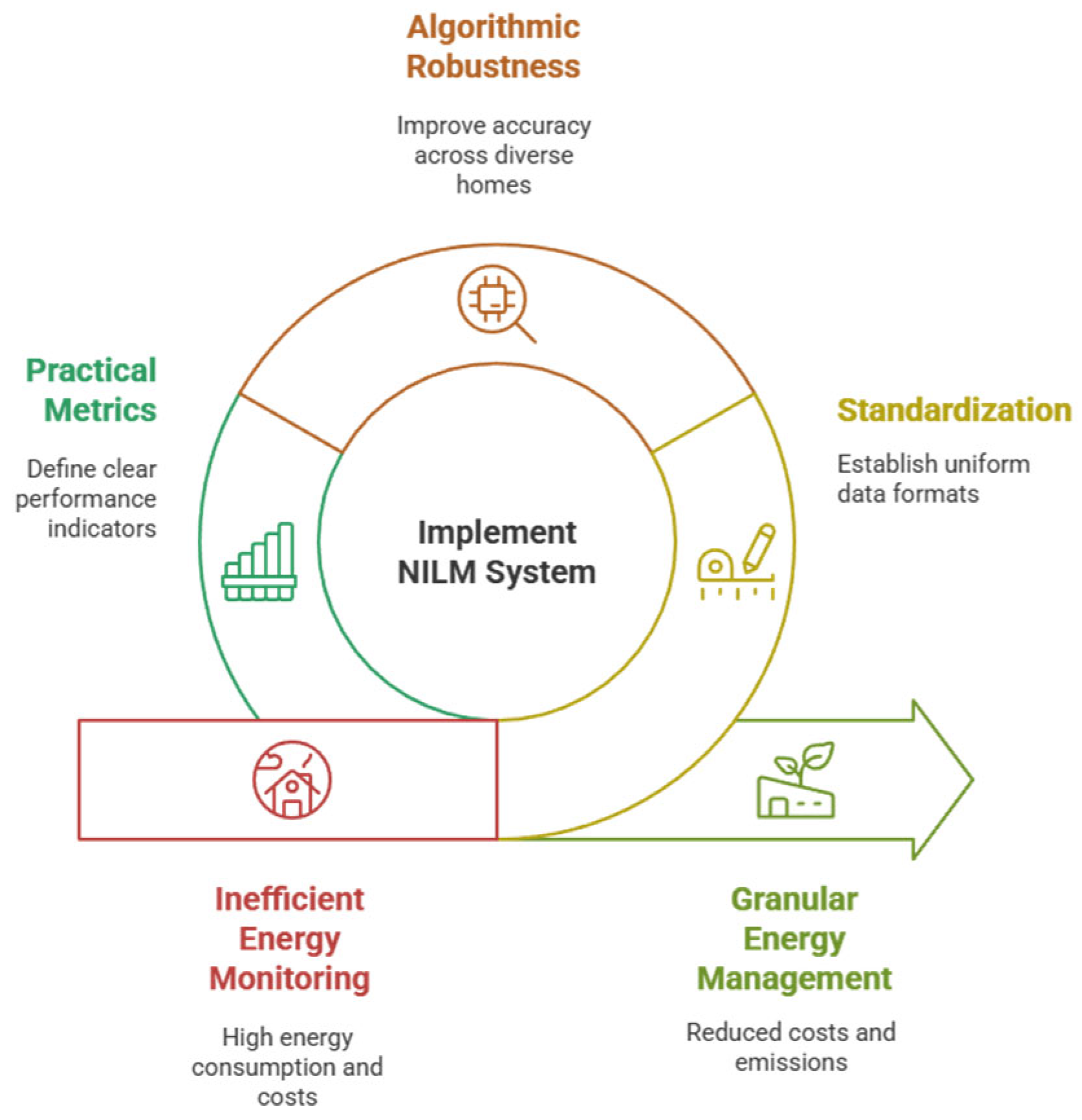
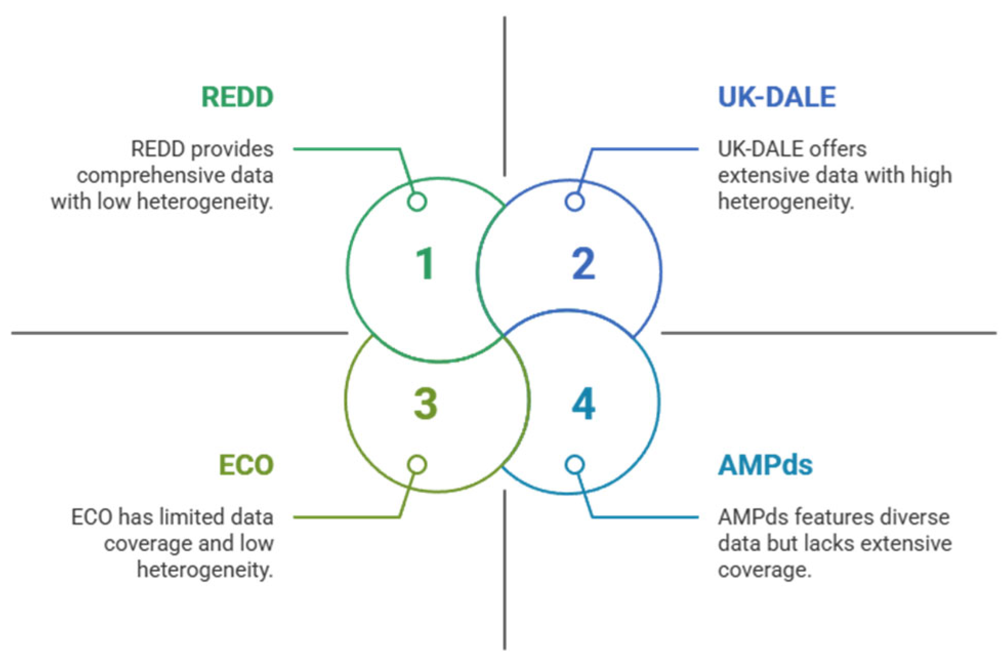
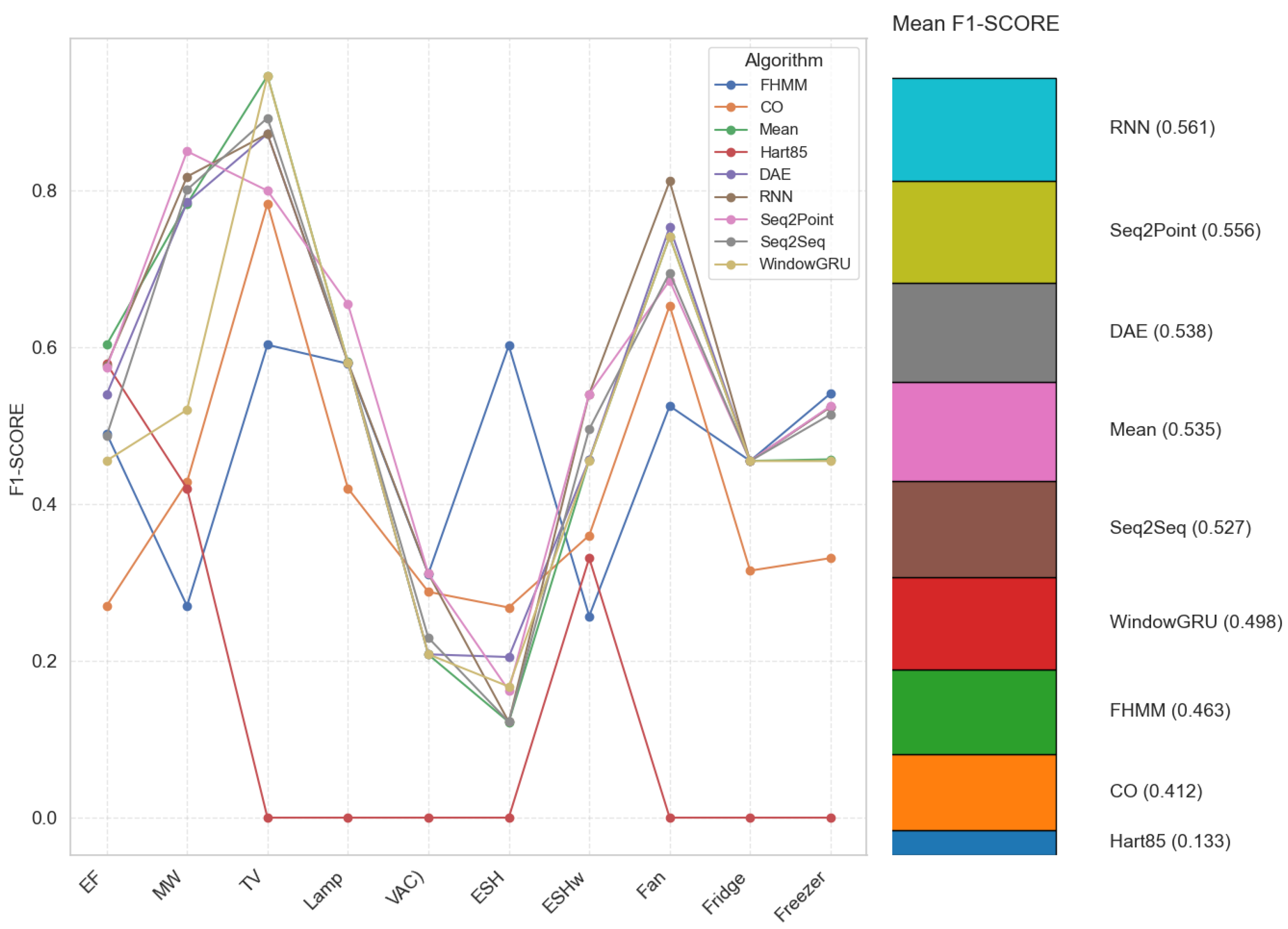
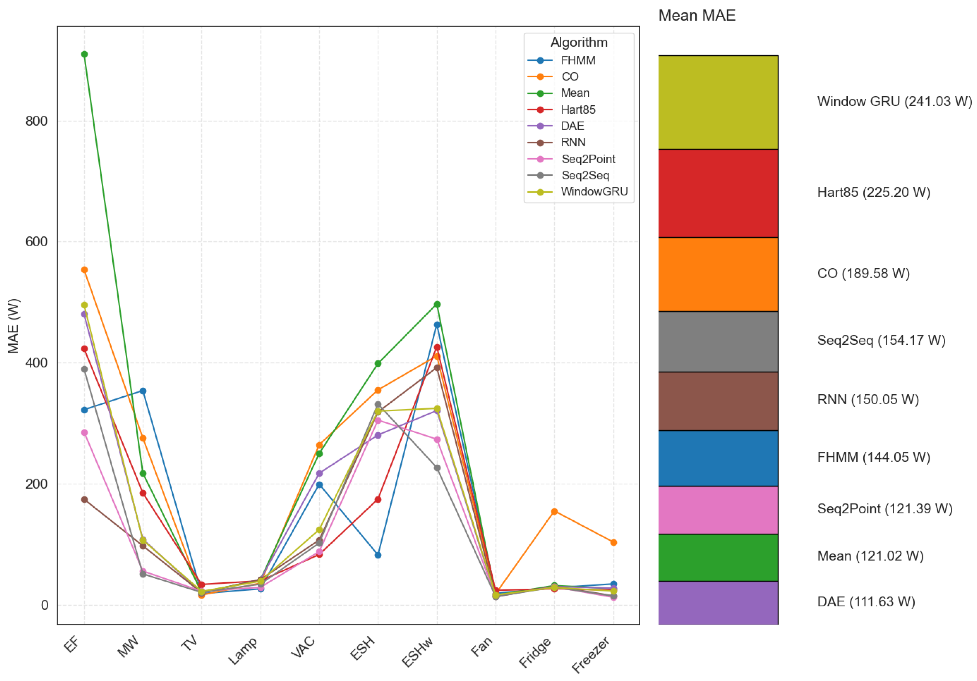


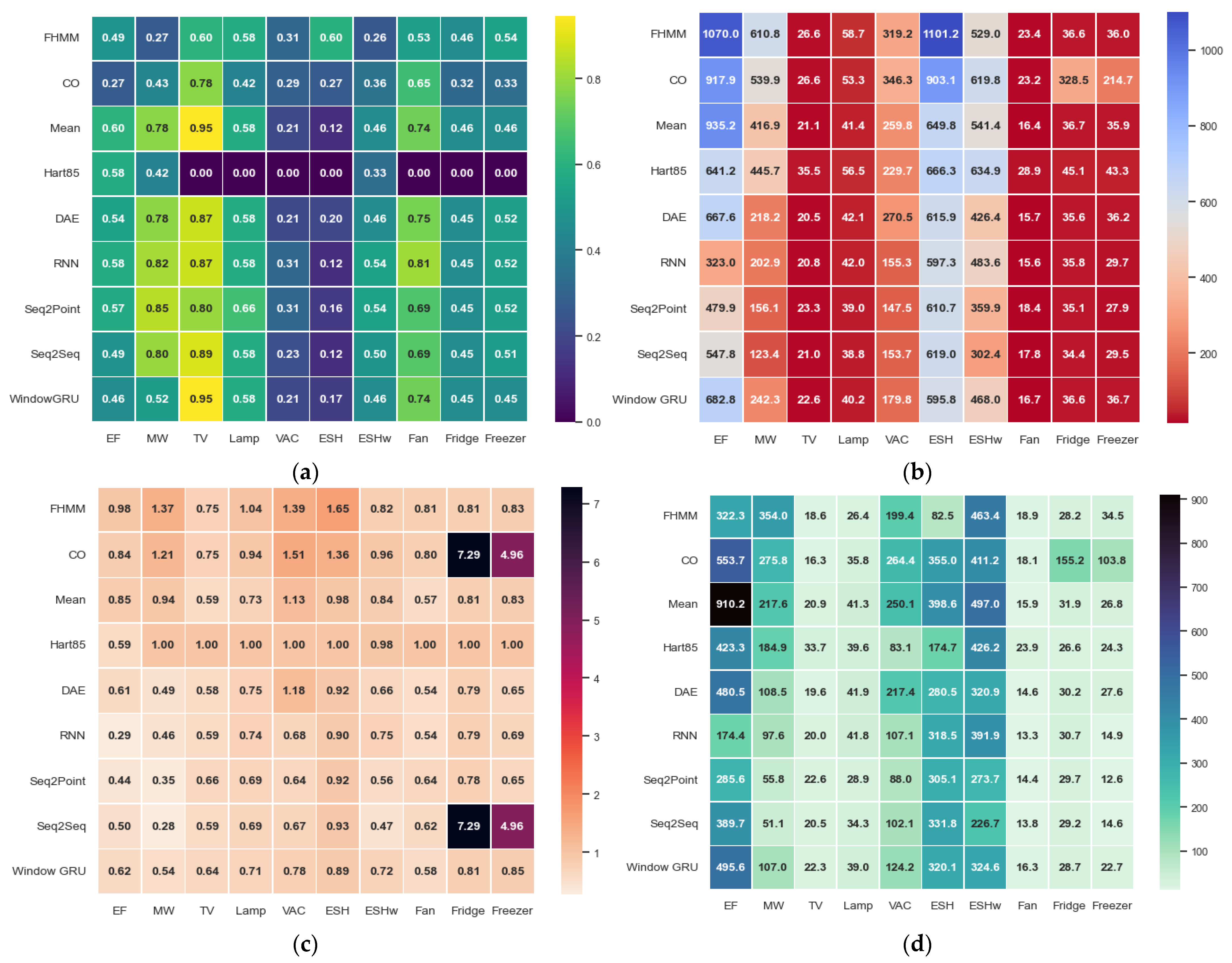
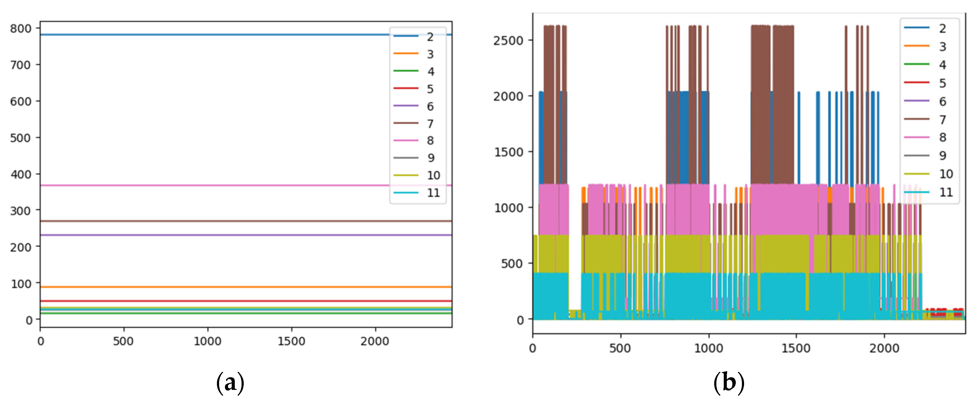

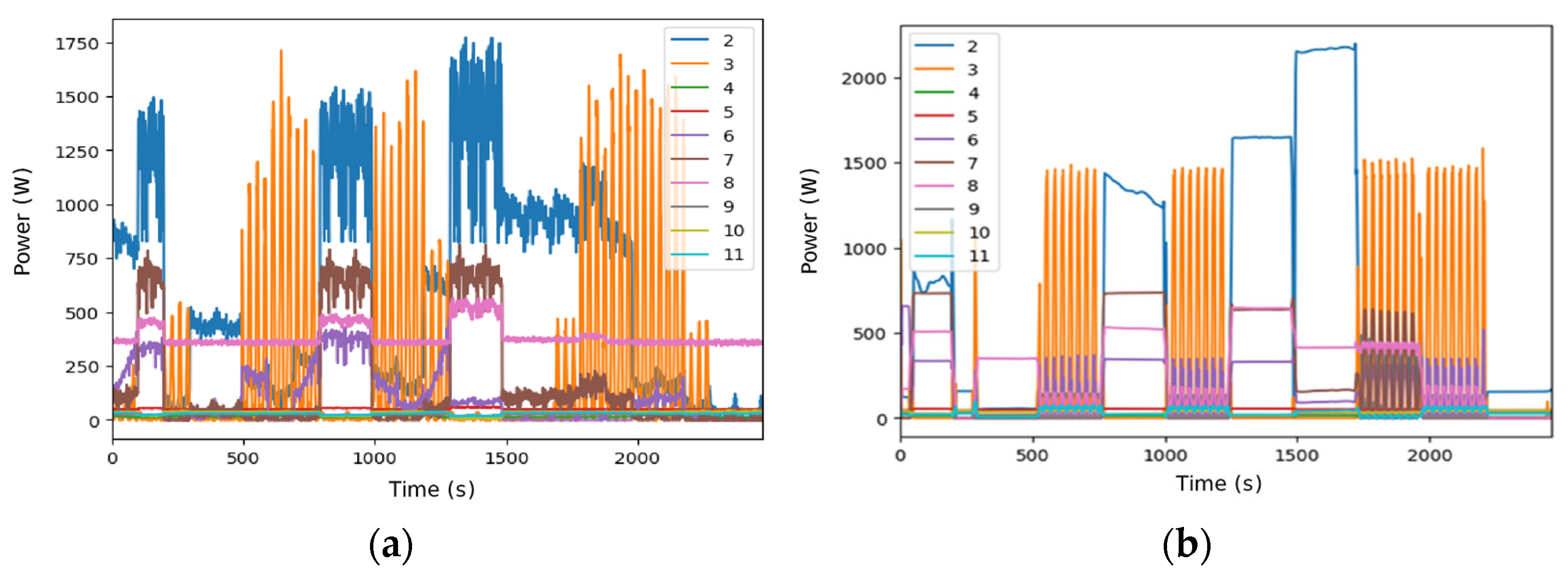

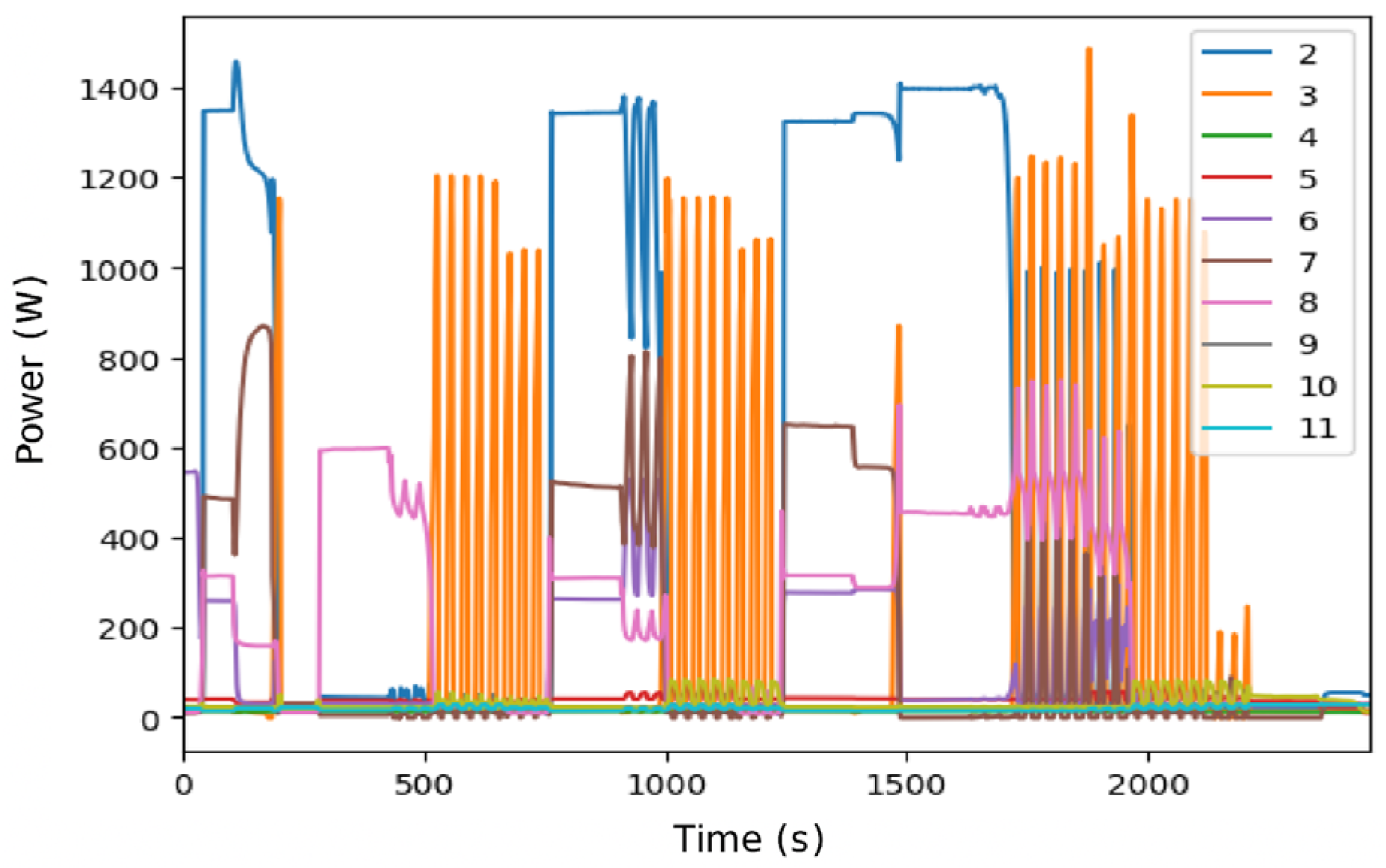
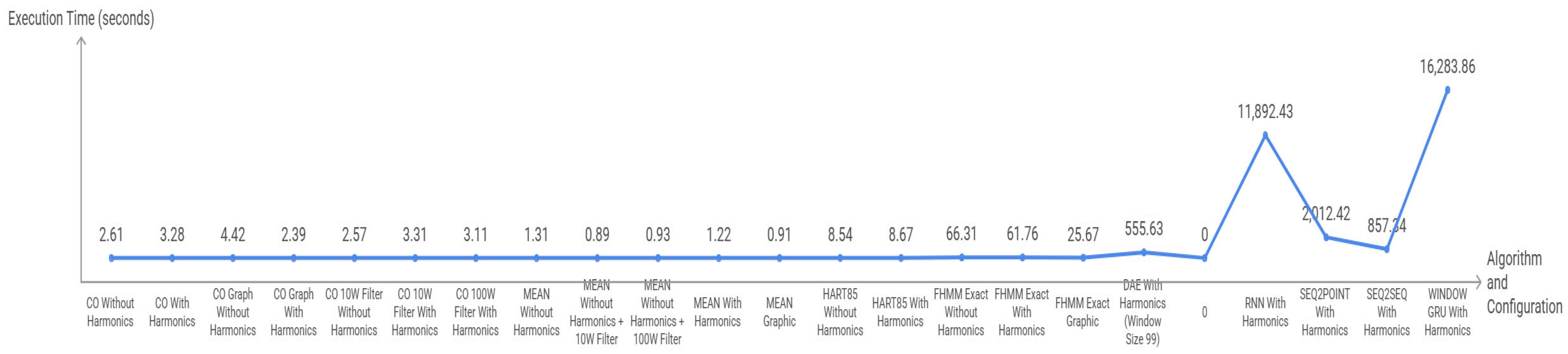
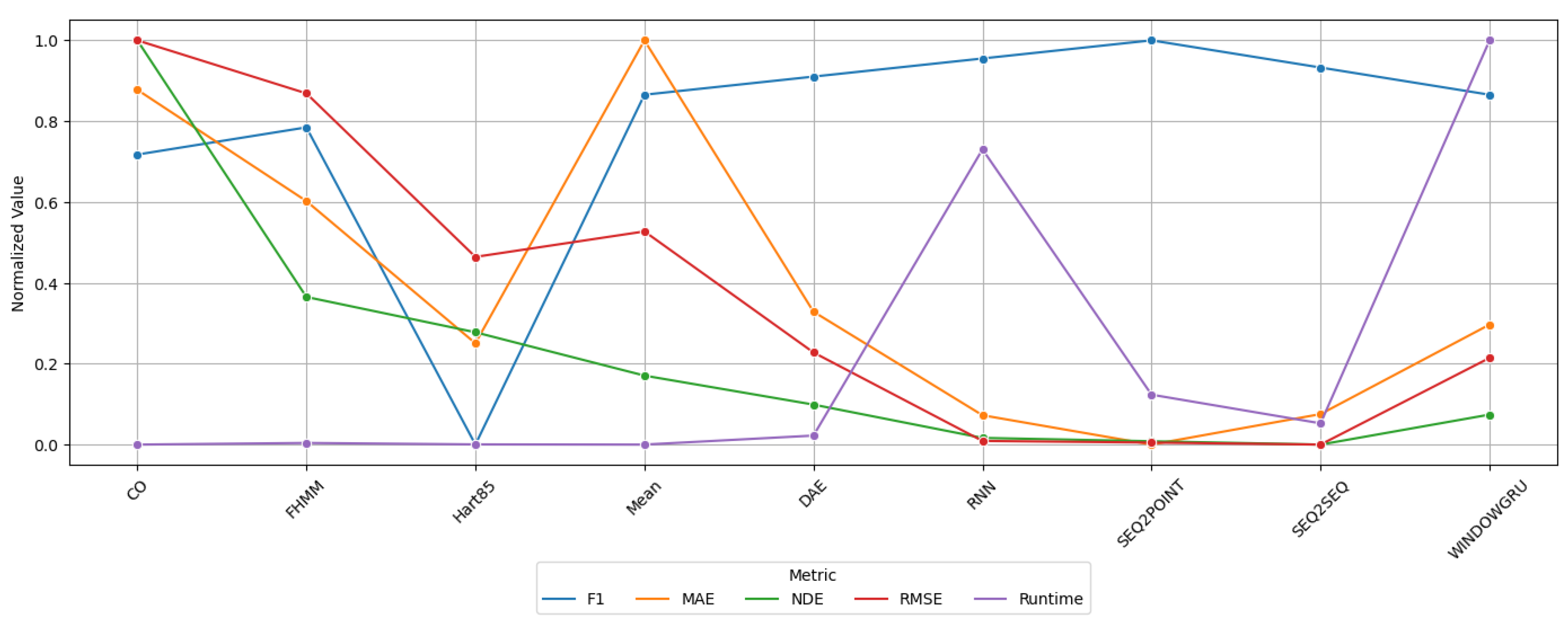
Disclaimer/Publisher’s Note: The statements, opinions and data contained in all publications are solely those of the individual author(s) and contributor(s) and not of MDPI and/or the editor(s). MDPI and/or the editor(s) disclaim responsibility for any injury to people or property resulting from any ideas, methods, instructions or products referred to in the content. |
© 2025 by the authors. Licensee MDPI, Basel, Switzerland. This article is an open access article distributed under the terms and conditions of the Creative Commons Attribution (CC BY) license (https://creativecommons.org/licenses/by/4.0/).