Automatic Phase Correction of NMR Spectra Using Brute-Force GPU Method

Abstract

Although there are still no fully guaranteed solutions to the problem of phase adjustment of NMR spectroscopy signals, it has not received much consideration recently, especially in the presence of noisy signals. To address this gap, we present a novel methodology, based on GPU processing, that is able to find the optimal parameter set for phase adjustment through an exhaustive search of all possible combinations of the phase space parameters. In our experiments, we were able to reduce the execution time of extensive GPU brute-force analysis to the same amount of time needed for the traditional CPU analysis, with the big advantage of searching all possible combinations on the GPU against just a few regions guessed by the CPU. In our case study, we also demonstrate the robustness of the proposed method with respect to the problem of local minima. Finally, we perform a Bland-Altman analysis to validate the entropies calculated using CPU and GPU processing for a set of 16 experiments from brain and body metabolites using 1H and 31P probes. The results demonstrate that our algorithm always find the globally optimal solution while previous CPU-based heuristics were stalled in a poor solution in 6.25% of a 16 sample universe.

1. Introduction

Proton NMR spectroscopy is a well-established and reliable diagnostic approach. It is commonly employed in conjunction with magnetic resonance imaging techniques, allowing physicians to compare anatomical and physiological alterations found in the metabolic and biochemical profile of a patient’s brain [1].

Transverse magnetization is the transverse component, relative to the B0 direction, of the macroscopic magnetization vector. The induction signal is generated by transverse rotary magnetization, and as the latter decays, induction also decays.

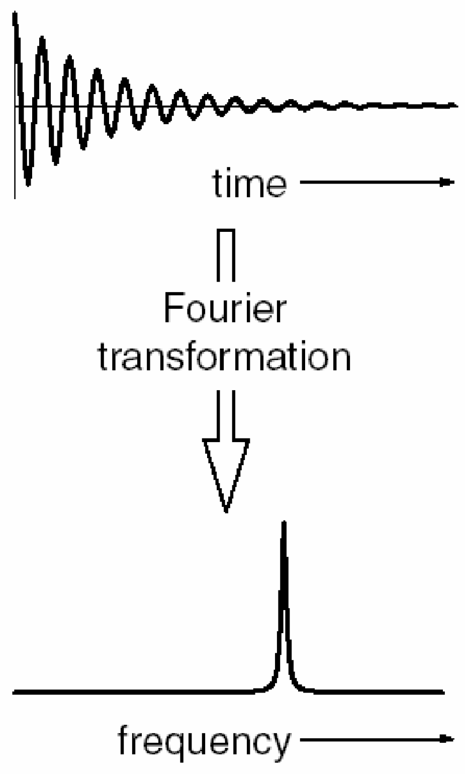
This relaxation action generates the free induction signal (where precession occurs at the Larmor frequency) called free induction decay or FID. FID is a signal that occurs when a radiofrequency (RF) pulse is turned off, causing protons to lose phase coherence. The FID signal is a sine wave that exponentially decreases in intensity until it reaches zero. The FID is a time domain signal (as shown in Figure 1), but to obtain the NMR spectrum, it is necessary to transform it to the frequency domain. To do this, a Fourier transformation (FT) of the FID is performed (Figure 2). The FID is important because it contains information about the NMR spectrum, which is useful in biological and biomedical research and applications.

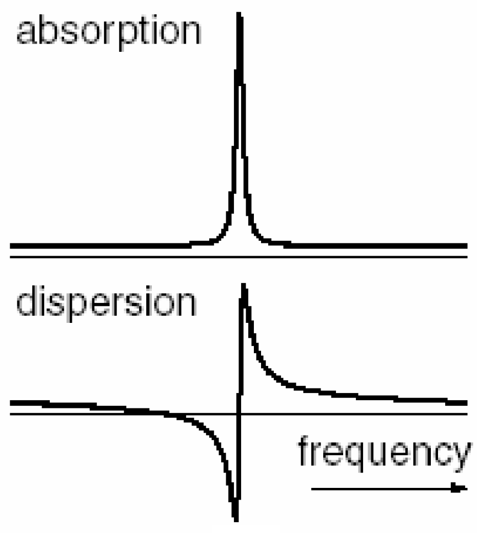
As seen in Figure 3, Lorentzian peaks form the real absorptive portion, where the imaginary is represented by the dispersive portion of the signal. The area of the absorptive part must tend to the maximum, whereas the area of the absorptivity must tend to zero, with the cancellation of the positive and negative parts.

The faster the FID decays, the wider the line in the spectrum corresponding (as shown in Figure 4). By integrating the lines in the spectrum, we can determine the relative number of protons (typically) contributing to each of them.

However, the signal may be phase-shifted, presenting a phase error. The traditional appearance of the spectrum depends on the position of the signal at time zero, e.g., the phase of the signal at time zero. There may be an unknown phase change, leading to a situation in which a clear absorption line is not shown in the real part, which makes spectral analysis difficult or even impossible. A phase adjustment can be applied to the spectrum, using different modes.

1.1. Phase Adjustment

Adjusting the phased spectra is a fundamental and necessary data post-processing step of the Nuclear Magnetic Resonance (NMR) methodology [2]. Nevertheless, after Fourier transformations, the initial spectra are not in pure absorption mode (Figure 5).

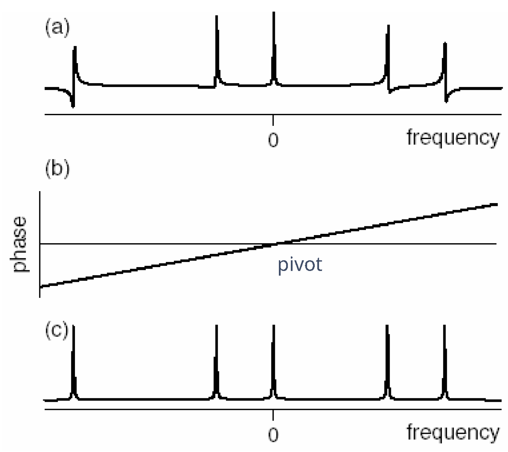
Normally, zero-order and first-order phase corrections are required for Fourier transform NMR spectra in order to obtain the desired appearance of the real part of the spectra. The zero-order phase misadjustment arises from the phase difference between the reference phase and the receiver detector phase. The first-order phase misadjustment arises from the time delay between excitation and detection, flip-angle variation across the spectrum, and phase shifts from the filter employed to reduce noise outside the spectral bandwidth. Zero-order phase correction is frequency-independent, while first-order phase correction is frequency-dependent [3].

If the offset becomes comparable with the RF field strength a 90° pulse about x results in the generation of magnetization along both the x and y axes. We can now describe this mixture of x and y magnetization as resulting in a phase shift or phase error of the spectrum [4], generating zero (PH0) and first (PH1) phase order correction factors.

Phase correction is the process of mixing the real and imaginary signals present in the complex spectrum of the free induction decay [5]. It is achieved by using a linearly changing phase correction angle along the spectrum, as determined by the following equation:

$$R_i=R_i^{0}cos\left({\varphi }_i\right)-I_i^{0}sin\left({\varphi }_i\right),$$

(1)

where $R_i$ is the ith point of the reference phased spectrum, $I_i^0$ is the ith point of the imaginary part of the unphased spectrum, $R_i^0$ is the ith point of the real part of the unphased spectrum, and ${\varphi }_i$ is the applied angle at point i.

In turn, ${\varphi }_i$ corresponds to a linear function of the position in the spectrum, defined as follows:

$${\varphi }_i=PH0+PH1\times {\displaystyle \frac{i-pivot}{N}},$$

(2)

where $PH0$ is the constant part of the phase angle (zeroth order correction), and $PH1$ is the total variation across the spectrum, consisting of n data points. It is important to note that the first data point is phased using angle $PH0$, while the last data point is corrected using angle $PH0+PH1$. All the points in between are calculated with a simple linear interpolation. Obviously, $PH0$ needs to be optimized only in the region of 0–${360}^{\circ }$ since both sine and cosine are the same for ${\varphi }_i$ and ${\varphi }_i+k\times {360}^{\circ }$, for integer k.

When a Fourier-transformed NMR spectrum is appropriately phased, the real part of the phased spectrum has only nonnegative spectral bands. In many ways, this is the most physically meaningful spectral representation. In contrast, the imaginary part possesses both the positive and negative extrema. Accordingly, only the entropy of the real parts of the phased spectra, considering $PH0$ and $PH1$, are considered in the objective function.

The objective function, possessing a Shannon type information entropy measure [6] for the phase correction problem, is shown in Equations (3) and (4):

$$minE=-\sum h_{i}ln{h}_i+P\left(R_i\right),$$

(3)

where h is the normalized derivative of the signal, P is a penalty function to ensure nonnegative bands in the spectrum, and m is the derivative order of the phased spectra [3]. In turn, $h_i$ is defined by Equation (4), as follows:

$$h_i={\displaystyle \frac{|R_i^m|}{{\sum }_i|R_i^m|}}.$$

(4)

1.2. NMR Data Processing

There has been less development of open source software for the analysis of NMR data than for MS (Mass spectrometry) [7]. It happens due to the majority of NMR spectrometers being supplied by only a few manufacturers. The software Top-Spin version 4.4.1 (Bruker BioSpin, Rheinstetten, Germany) which comes bundled with Bruker instruments, is the most widely used tool for NMR data preprocessing [8].

Most of the free software that is available for use is written in MATLAB version 9 or superior (e.g., Dolphin [9], FOCUS [10] and MatNMR [11]), restricting their use to those with access to this commercial software. Gradually MATLAB based tools are being ported onto freely available platforms like Icoshift [12], a versatile tool for the rapid alignment of 1D NMR spectra which now has a Python implementation (mfitzp/icoshift).

The only open software whose use was reported in the Metabolomics Society survey for NMR preprocessing was rNMR [13], which uses a regions of interest (ROIs) based approach for the analysis of 1D and 2D NMR spectra.

2. Methods

The problem that occurs when performing spectra phase correction using entropy minimization techniques lies in the fact that the minimization methods—such as the least squares method—are subject to errors due to the occurrence of local minima in their search space, which is particularly common with noisy signals.

It is necessary, therefore, to find the best set of parameters to efficiently perform the spectra phase correction. The straightforward approach would be to test each possible combination of $PH0$, $PH1$, and the pivots (pivot is the $PH1$ offset related to the spectra length). This strategy is computationally expensive, so not practical for CPU-based approaches. Instead, we opt for a GPU-based approach to find the best parameters by exhaustively testing the search space defined by such parameters.

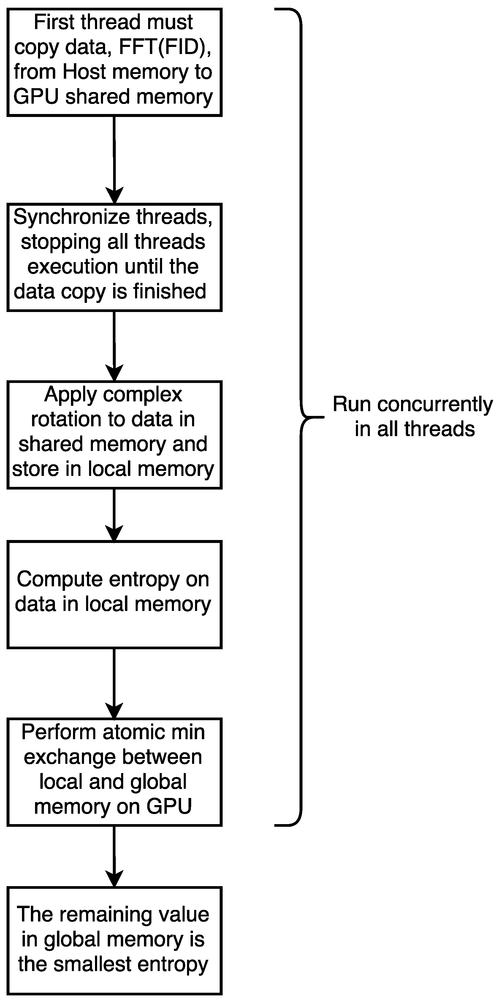
For the GPU version of our code, Figure 6 shows the parallel approach used to implement this solution; the complete source code is available in an open-source repository [14]. For the CPU version, we chose a Matlab library called MatNMR [11].

The Listing 1 presents the CPU code used to compute the entropy minimization using the least-squares method with a single pivot. Based on the same software Python (version 2.7) development framework we developed our GPU version with the launch script shown in Listing 2. The remaining code is available at our Github repository [14]. The goal was to evaluate the performance of entropy minimization on a GPU, considering all possible pivots as well as all PHC0 and PHC1 factors.

Listing 1. Matlab script to evaluate the CPU entropy (for a single pivot) using the least squares method provided in library MatNMR [11].

Listing 2. Python script to evaluate the CPU entropy (for all the pivots) using the least squares method.

3. Results

In our experiments, we were able to reduce the execution time of the extensively GPU brute-force analysis to the same time of traditional CPU analysis with the big advantage of searching all possible combinations in GPU against only a few regions guessed by CPU.

We used an NVIDIA Titan XP GPU with 3840 cores running at 1.58 GHz with 12 GB of G5X memory. Our CPU was an Intel (Skylake) Celeron (Santa Clara, CA, USA) with two cores running at 2.80 GHz and 16 GB of DDR3 memory. Philips (Amsterdam, The Netherlands) Achieva 3T equipment was used to generate all the spectra. There was neither optimization nor zero-filling on the acquired data before performing the standard fast Fourier transformation.

Table 1. Phase adjustment results: (I) CPU Entropy minimization by least squares (as proposed by Chen et al.) [3]; (II) Brute-force entropy analysis using GPU-based processing.

	Entropy (MinE)	Order 0 (PH0)	Order 1 (PH1)	Pivot (i)
I (CPU processing sample E from Table 2)	7.329	−10.6	42.4	779
II (GPU processing sample E from Table 2)	7.312	73.0	−127.0	1137

shows the entropy results for our noisier data spectrum (2048 points).

Table 2. Spectra details and indication if CPU and/or GPU finds the optimal global solution.

#	Sample	Isotope	Band	TE/TR	Size	CPU Global	GPU Global
01	A	1H	3155 Hz	32/3700 ms	8192	YES	YES
05	B	1H	1725 Hz	35/1500 ms	2048	ALL	ALL
01	C	1H	2000 Hz	58/2000 ms	1024	YES	YES
02	D	1H	2000 Hz	288/2000 ms	1024	ALL	ALL
01	E	1H	1725 Hz	135/1600 ms	2048	NO	YES
02	F	1H	1500 Hz	25/1600 ms	2048	ALL	ALL
01	G	1H	1800 Hz	36/1800 ms	2048	YES	YES
01	H	31P	2225 Hz	0.1/3500 ms	1024	YES	YES
01	I	31P	2225 Hz	0.1/3500 ms	1024	YES	YES
01	J	1H	1500 Hz	60/1600 ms	2048	YES	YES
16

Sample A: 1H spectrum of a phantom with 8192 points. Samples B: 1H spectra of the same phantom but with 2048 points. Sample C: In vivo 1H spectrum acquired from human liver. Samples D: In vivo 1H spectra acquired from the cingulate gyrus region of the human brain. Sample E: In vivo 1H spectrum acquired from the hippocampal region of the human brain. Samples F: In vivo 1H spectra acquired from human marrow. Sample G: In vivo 1H spectrum acquired from human muscle. Sample H: 31P spectrum acquired from the occipital region of the human brain. Sample I: 31P spectrum acquired from human muscle. Sample J: 1H spectrum of a phantom for fat quantification. *All spectra were acquired with a 3 T magnetic field.

presents the other features for this spectrum. Figure 7 depicts the results after the CPU and GPU phase adjustments.

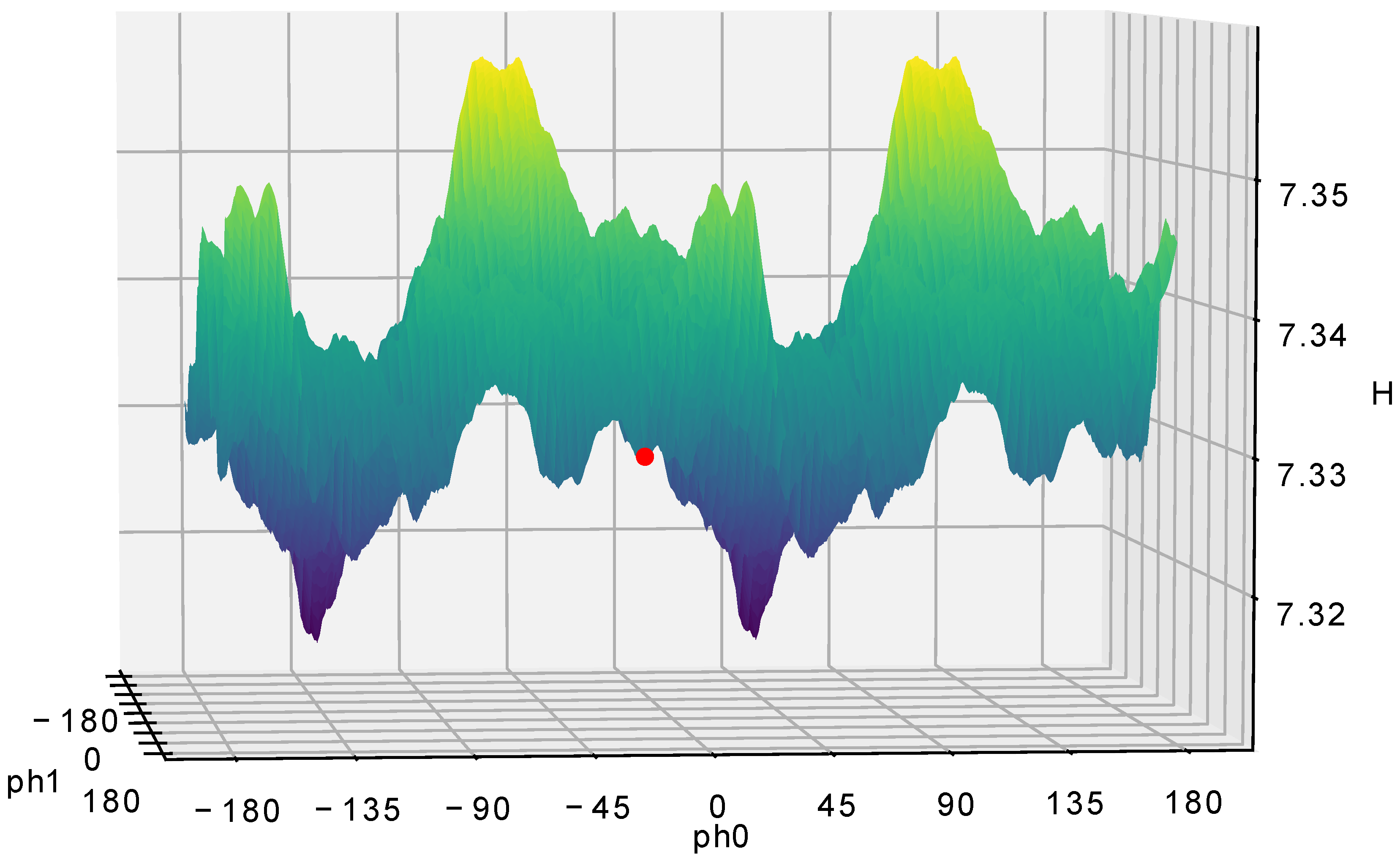
Figure 8 and Figure 9 depict the entropy maps. Here, the critical observation, as shown in the figures, is that the CPU-based method found a local minimum, while the GPU-based method found the global minimum. There is an obvious periodic symmetry on PH0 axis since it is linearly independent. We keep both sides in our calculations to illustrate the searching through the phase space completely. However, due to nature of PH1 relation with the pivot there is no periodic symmetry on this axis.

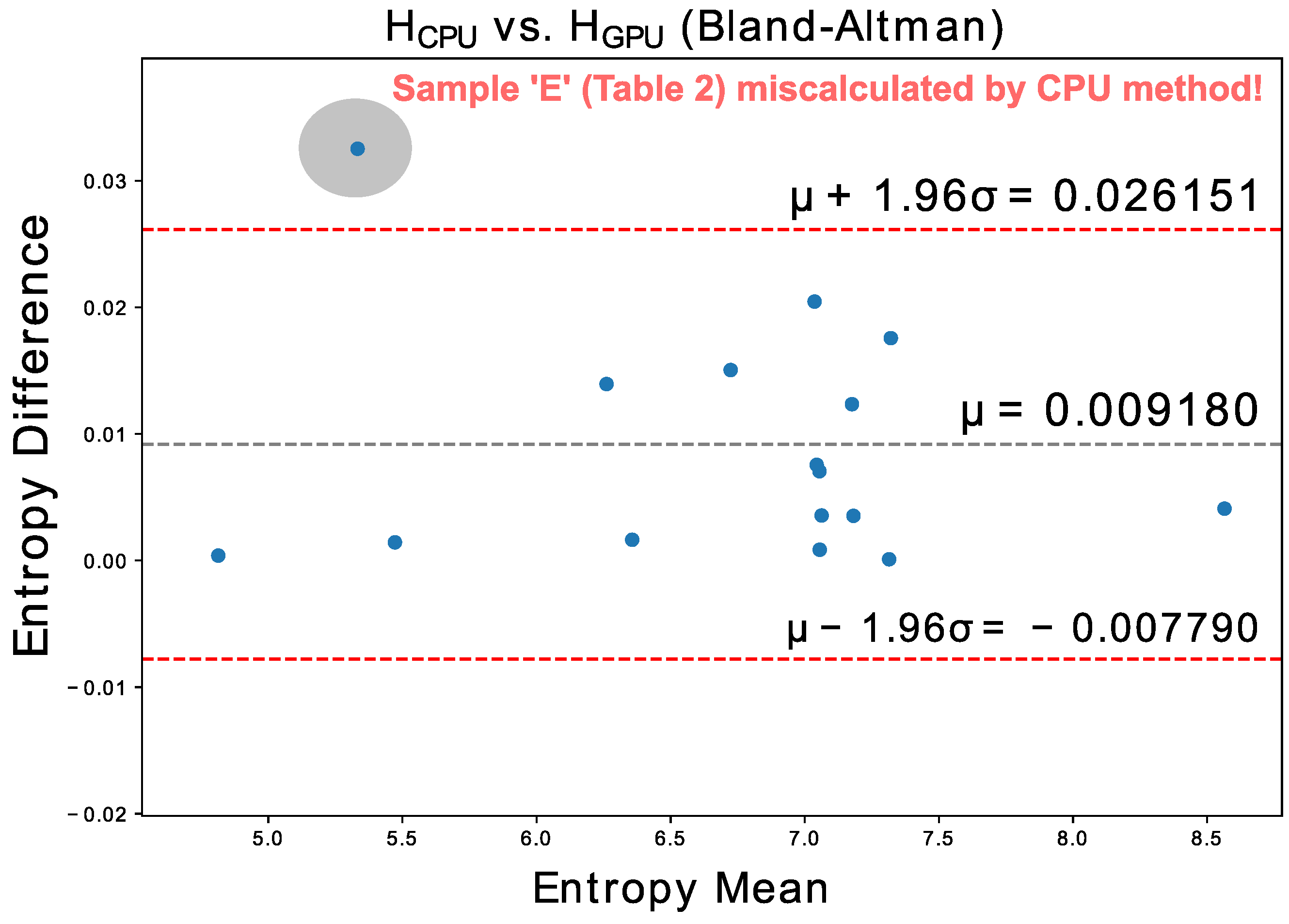
We performed an additional fifteen acquisitions with 1H and 31P probes in regions such as the cingulate cortex, occipital lobe, muscles, liver, and bone marrow; including several phantoms to test temporal stability. Their entropies, evaluated both with the CPU and GPU algorithms, are compatible according to the Bland-Altman plot presented in Figure 10.

For these sixteen samples the GPU algorithm run about 3.3 times faster than the CPU algorithm (even performing the brute force search, which is much more exhaustive), with the GPU being correct in all exams, and the CPU being wrong in one of them, that is, an error of 6.25% for a universe of 16 samples.

4. Discussion

We conclude that the advent of GPUs, with their massive parallel-processing capabilities, allows us to perform techniques that were impractical in the recent past, such as scanning all the possibilities of a phase space (including all the pivots). This opportunity translates into finding the best solution for the phase adjustment problem in Nuclear Magnetic Resonance spectroscopy.

In comparison to commercial software, where the pivots are set manually, the user needs to test thousands of pivot points to expand the search space—without the guarantee of finding the optimal results, since traditional CPU analysis suffers from risk of local minima stall, even with manually setting of the pivot.

In general, our GPU brute force search method works fine even with anomalous spectrum like multiplets and inverted peaks, since the ideal position of pivot can solve this issues by turn negative peaks into positive ones. Multiplets, on the other hand, could also be enhanced in further spectroscopy stages.

Some other possible aspects of the signal, such as overlapping peaks in the spectra, need to be processed in the later stages of the spectroscopy, using techniques other than phase adjustment, and were not within the scope of the present work.

Thus, by using brute force techniques in GPU technology, we developed a more robust method, which is capable of solving this optimization problem more efficiently and effectively, always finding a global minimum without the risk of stalling at local minima, as previous CPU-based methods were subject to.

References

- Ramin, S.A.L.; Tognola, W.A.; Spotti, A.R. Proton magnetic resonance spectroscopy: Clinical applications in patients with brain lesions. Sao Paulo Med. J. 2003, 121, 254–259. [Google Scholar] [CrossRef] [PubMed]
- Neff, B.; Ackerman, J.; Waugh, J. Fully automatic software correction of fourier transform NMR spectra. J. Magn. Reson. (1969) 1977, 25, 335–340. [Google Scholar] [CrossRef]
- Chen, L.; Weng, Z.; Goh, L.; Garland, M. An efficient algorithm for automatic phase correction of {NMR} spectra based on entropy minimization. J. Magn. Reson. 2002, 158, 164–168. [Google Scholar] [CrossRef]
- Keeler, J. Understanding NMR Spectroscopy; University of Cambridge: Cambridge, UK, 2004; Volume 1, Chapter 4; pp. 4.1–4.18. [Google Scholar]
- de Brouwer, H. Evaluation of algorithms for automated phase correction of NMR spectra. J. Magn. Reson. 2009, 201, 230–238. [Google Scholar] [CrossRef] [PubMed]
- Shannon, C.E. A mathematical theory of communication. Bell Syst. Tech. J. 1948, 27, 379–423. [Google Scholar] [CrossRef]
- Spicer, R.; Salek, R.M.; Moreno, P.; Cañueto, D.; Steinbeck, C. Navigating freely-available software tools for metabolomics analysis. Metabolomics 2017, 13, 106. [Google Scholar] [CrossRef] [PubMed]
- Weber, R.J.; Lawson, T.N.; Salek, R.M.; Ebbels, T.M.; Glen, R.C.; Goodacre, R.; Griffin, J.L.; Haug, K.; Koulman, A.; Moreno, P.; et al. Computational tools and workflows in metabolomics: An international survey highlights the opportunity for harmonisation through Galaxy. Metabolomics 2017, 13, 12. [Google Scholar] [CrossRef] [PubMed]
- Gómez, J.; Brezmes, J.; Mallol, R.; Rodríguez, M.A.; Vinaixa, M.; Salek, R.M.; Correig, X.; Cañellas, N. Dolphin: A tool for automatic targeted metabolite profiling using 1D and 2D 1 H-NMR data. Anal. Bioanal. Chem. 2014, 406, 7967–7976. [Google Scholar] [CrossRef] [PubMed]
- Alonso, A.; Rodríguez, M.A.; Vinaixa, M.; Tortosa, R.; Correig, X.; Julià, A.; Marsal, S. Focus: A Robust Workflow for One-Dimensional NMR Spectral Analysis. Anal. Chem. 2014, 86, 1160–1169. [Google Scholar] [CrossRef] [PubMed]
- van Beek, J.D. matNMR: A flexible toolbox for processing, analyzing and visualizing magnetic resonance data in Matlab®. J. Magn. Reson. 2007, 187, 19–26. [Google Scholar] [CrossRef] [PubMed]
- Tomasi, G.; Savorani, F.; Engelsen, S.B. icoshift: An effective tool for the alignment of chromatographic data. J. Chromatogr. A 2011, 1218, 7832–7840. [Google Scholar] [CrossRef] [PubMed]
- Lewis, I.A.; Schommer, S.C.; Markley, J.L. rNMR: Open source software for identifying and quantifying metabolites in NMR spectra. Magn. Reson. Chem. 2009, 47, S123–S126. [Google Scholar] [CrossRef] [PubMed]
- Gazziro, M. AutoML_GPU. 2024. Available online: https://github.com/mariogazziro/AutoML_GPU/tree/master/phase_adj (accessed on 17 January 2025).