Power-Hardware-in-the-Loop Simulation for Applied Science, a Review to Highlight Its Merits and Challenges

Abstract

The last thirty years have brought an evolution of electrical power systems. The integration of renewable energy and energy storage, dynamic loads, or distributed resources based on power electronics, including communications systems and protocols, is usual. Fortunately, technological advances have also brought tools to face the complex field of electrical component integration to the power system, such as the real-time power-hardware-in-the-loop (PHIL) simulation. This paper argues why PHIL simulation is a mighty tool for addressing intelligent design, modeling, and computing methods to address complex power systems. Nevertheless, any promising technology can be misunderstood, reducing its positive effect. This article uses two inverters connected to a microgrid to develop the steps from conceptualizing an idea to a PHIL simulation, highlighting the merits, drawbacks, and lessons learned. Two perspectives are developed. First, the multiple, even complex, details required for furnishing a PHIL simulation are described. Second, reflections on how PHIL simulations enhance the scientific impact of the research compared to offline simulations or scale prototypes are made, enabling the transition from academic to applied research to attend to the challenges of modern power systems. The successful results of the microgrid PHIL simulation are shown to prove the merits of this approach.

1. Introduction

Century XXI is the age of real-time simulation, which is conspicuously used in power system research and the development of new knowledge [1,2,3,4]. The current power systems are interconnected to myriads of power converters, which address multiple applications, including active filters, custom power devices, HVDC converters, induction motor drives, and, lastly, grid-forming inverters (GFMIs) and grid-following inverters (GFLIs) in microgrids. Fortunately, these developments are a consequence of a historic and ordered development of the electrification process [5,6].

Despite the high level and amount of research developed following the real-time simulation procedures, flawless results are only sometimes achieved for electrical facilities [7]. This is a typical situation when relatively new high technology advances into the main applications of a complex field such as modern power systems [4,8,9,10,11].

For instance, in [1], the authors present an interesting development of a Power-In-The-Loop (PHIL) simulation for a residential microgrid. However, software and hardware interconnection details need to be recorded to ensure the reproducibility of the experiments using real-time simulators.

Reference [12] is an excellent article that thoroughly shows the details of evaluating a commercial microgrid interconnection using PHIL simulation. Other papers carefully record the interconnection details associated with PHIL simulation [2,13,14]. This is relevant since it provides significant information for reproducing the PHIL simulation.

There are thesis works devoted mainly to interconnection schemes for different applications that are very valuable for consideration [15]. Likewise, there are multiple papers in the current and old state-of-the-art related to microgrids and PHIL simulations, as can be read in [16,17,18,19]. Previous articles reveal that real-time PHIL simulation can provide relevant conclusions with an enhanced approach to the real world and reduced costs.

The article [20] analyzes the capability of performing PHIL scenarios related to extreme conditions. The authors perform a PHIL simulation of a microgrid to be applied to a Lunar Habitat. Imagine the criticality of those kinds of results based on PHIL simulation. Another type of article that performs PHIL simulations to demonstrate the feasibility of implementing emergent developments can be consulted in [15,21] in which the authors pose the reaction of a microgrid against cyber-attacks, providing relevant results to be considered in that field of knowledge. This evolution has motivated the formulation of novel concepts of testing and prototyping, such as digital twins [22,23,24,25]. Consequently, with the development of technology, artificial intelligence also plays a role in the electrical world [26].

PHIL simulation is also a powerful tool for power electronics. It enables the assessment of converters by utilizing metrics derived from the actual device rather than relying on those provided by the models. In the article [27], the authors evaluate control algorithms for power electronics using statistical methods. PHIL simulation offers improved approximations, enhancing the study of the reliability of power electronics converters. However, achieving accurate results requires robust interconnection models that ensure the stability of the PHIL simulation. There is also ongoing research into automatic control schemes in the interconnection model to address this need [28,29,30,31].

Considering the vast amount of information related to real-time simulations and their different applications, this article aims to provide an organized insight by stages about building from model conceptualizations and offline simulations to real-time PHIL simulations considering the following bullets:

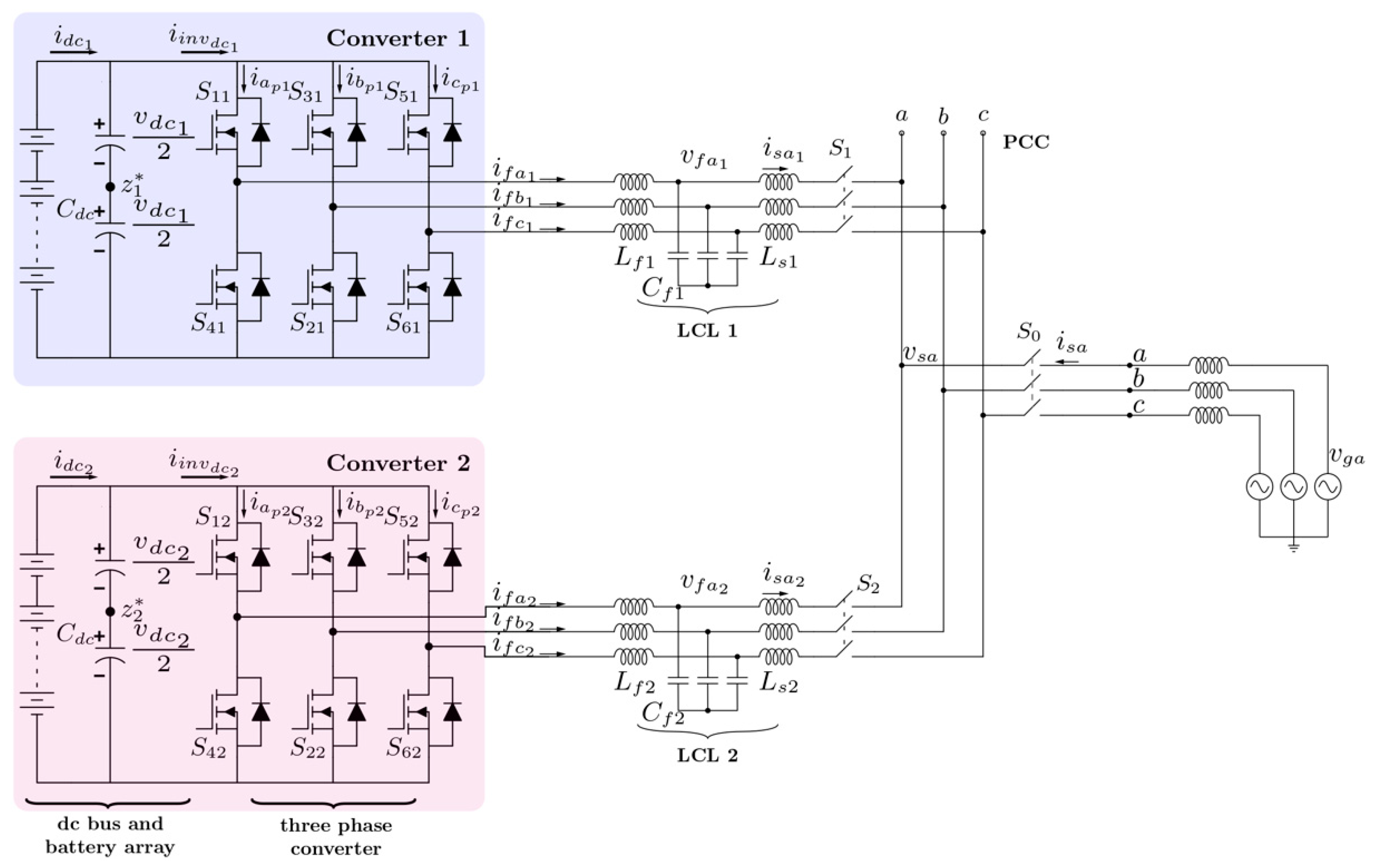
• A microgrid based on two inverters connected to an equivalent grid is used as a study case.
• Reflections from basic model conceptualization to be simulated offline are addressed.
• To aid in the process, considerations about the capability of the offline simulation to furnish the real-time simulation are argued.
• Insights on the relevant aspects of the implementation of the PHIL simulation are addressed and commented on.
• The advantages and drawbacks, as well as the lessons learned during the process, are discussed.
• The merits of PHIL simulation are explained by the results obtained using OPAL-RT-based microgrid experiments.

The reference [32] is a previous work where the author of this article actively participated in obtaining a microgrid result in PHIL simulations, and the reflections and insight obtained, as well as some results, are used to write this paper with a different scope.

Once the purpose of this article has been established, the following sections will be described: Section 2 is devoted to selecting the subject under study in this case, and it shall briefly describe the simulation setup based on the selected microgrid. Section 3 explains each stage of real-time simulation, from equations to PHIL simulation, reflecting on each stage’s merits and drawbacks, arguing the kind of research each stage permits, and the lessons learned. Finally, in Section 4, a discussion of the article is presented.

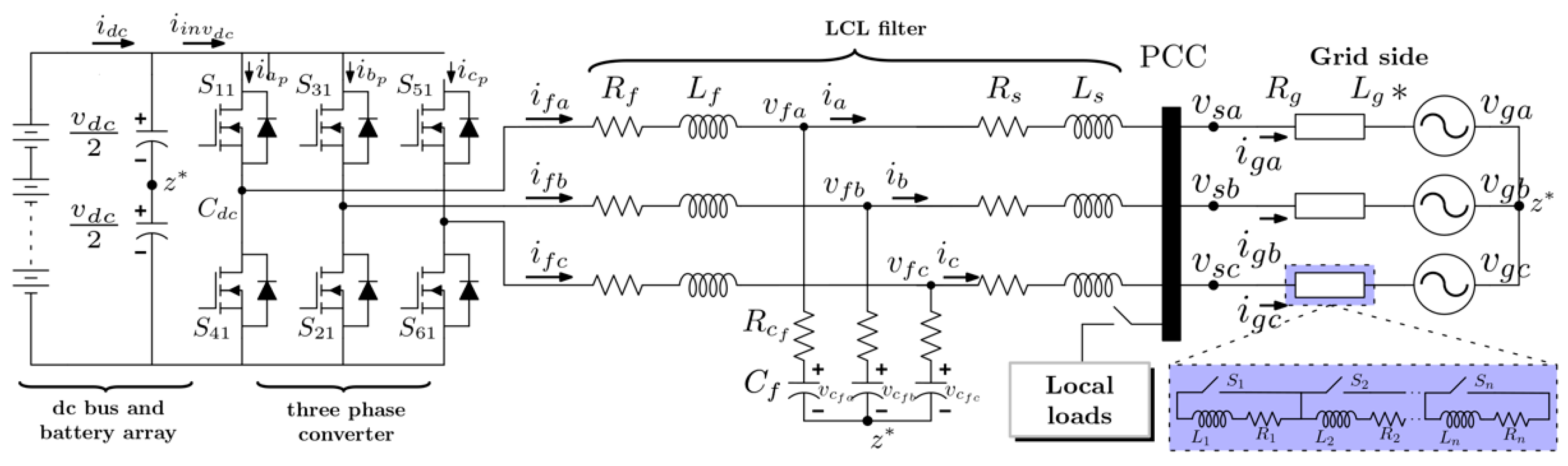
2. Selecting the Study Object

Real-time simulation should be seen as more than a powerful tool that can be mechanically used. Its capabilities permit it to conceive enhanced scenarios, demonstrating that basic research can advance faster toward applied research. Figure 1 introduces a flow diagram to describe the process from a conceptualized scientific idea to the real-time PHIL simulation. The flowchart presented in Figure 1 is valuable because it aids in conceptualizing real-time power-hardware-in-the-loop (PHIL) simulations for systems with complex, risky, or costly physical implementations. By following the steps outlined in the flowchart and utilizing real-time PHIL simulators based on platforms such as OPAL-RT, RTDS, Typhoon, DSpace, or any other accessible resources, researchers can enhance their work with improved demonstrations, approximations, and arguments that contribute to advancements in knowledge. This article focuses on the OPAL-RT platform, which is the laboratory’s available resource for conducting PHIL simulations. While this equipment represents a significant innovation for designing multiple tests and improving modeling, transitioning from mathematical conceptualization to operational PHIL formulation involves several key aspects worth addressing. These considerations will help new researchers learn and deepen their understanding of the real-time PHIL simulation platform they have at their disposal.

This diagram illustrates the flow alongside three main dotted blocks. The red dotted line shows those parts that can be simulated offline or in real time. The purple dotted line shows the part suggested for real-time simulation. The green dotted line shows the part that can be performed in real-time PHIL simulation. Each dotted colored box contains bullet points with comments that shall be developed in the following sections. From a scientific standpoint, any system can be a candidate to be tested by a real-time PHIL simulation. In the context of this article, the scenery selected to give details that explain the significance of the real-time PHIL simulation is a microgrid whose scheme is shown in Figure 2.

The microgrid settings were selected to demonstrate the integration capability of the PHIL simulation using OPAL-RT. Then, the parameters of the power inverter shown in Figure 2 are as follows:

• L_f1 = 1.15 mH, L_s1 = 393 µH, C_f = 4.7 µF;
• L_f2 = 3.33 mH, L_s2 = 532.5 µH, C_f2 = 10 µF;
• v_gx = 30 V_peak with x = a, b, c;
• v_dc = 120 V;
• f_n = 50 Hz, grid frequency;
• m_f = 41, frequency index modulation;
• f_sw = 2050 Hz, switching frequency;
• Step time = 20 µs; integration step.

The control objective of the microgrid, just for illustrative purposes, is the interchange of active, reactive, and apparent power between the inverters and the grid.

Figure 2 scheme shall be used for arguing purposes in the following sections, and the results of the PHIL simulation shall be shown in Section 3.4.

3. Stages of the Real-Time Simulation

As a general assumption, consider that all the following developments and comments refer to an OPAL-RT platform for real-time simulation.

3.1. Basic Concepts

At the beginning of the process, having the north well recognized on the horizon of the real-time simulation purpose is relevant. This means the following:

• Select the study object: The plant and its constitutive parts should already be selected and parameterized.
• Electrical specification of the system: The purpose of the plant should be established, preferably with a clear scope of the functions and operation modes related to a known specification or recommendation. This will allow for the establishment of clear control objectives.
• Decide the modeling; does it work for your purposes? This part is the beginning of reaching a PHIL simulation; therefore, although it does not provide different information than offline simulations, it permits the recognition of the initial real-time simulation problems to be overcome.

Figure 3 shows the general structure of the simulation at the first stage. The center of the figure is the plant, highlighted in green.

Once this plant has been selected, in this case, the inverters of the microgrid and their functions are established, and then the conceptualization of the modeling to be used as the first approach can be made. For instance, in this article, the plant is a three-phase power inverter modeled in state space. The modeling can consider delta, star, or single-phase per-phase modeling depending on the research objectives. On the left of Figure 3 is the block “control system”, highlighted in purple. Depending on the research purposes, that block can include any kind of controller, linear or non-linear, or intelligent controllers. On the right of Figure 3 is the block “User Interface”, where the calculus of references and signals deployment can be carried out.

In this simulation stage, the fundamental concepts can be conceptualized and formulated as a valuable piece of the program to be tested. Considering this standpoint, within the plant block, three space state models are selectable depending on the features of the desired simulation. The first one is obtaining a three-phase, delta-connected, state space model. The second is obtaining a three-phase, star-connected, state space model, and the final is obtaining a single-phase line to neutral state space model. Each one can provide different information according to the purpose of the experiment. For example, a star-connected model could be preferred if unbalanced conditions were considered in the formulation process. Another different situation can be formulated, for instance, if some kind of research is desirable to be addressed with special consideration to the decoupled response of each leg of the converter. In that case, a single-phase model for each phase can be better. In this way, this stage pretends to illustrate the relevance of building a solid base to stimulate the creative process of specialized research. Consider

Table 1. Merits and drawbacks of the stage 1, basic concepts.

Merits
Allows one to demonstrate the model’s feasibility. There is flexibility depending on the purpose of the research, so the modeling of each converter can be carried out in delta-connection, star-connection, or single-phase per phase. The average modeling can provide relevant information about the plant such as eigenvalues locus, stability of the system, bandwidth, and transitory response. Allows one to formulate, depending on the modeling structure, control schemes in a straightforward way. The simulation is relatively easy to perform.
Drawbacks
This simulation provides the lowest precision since it is based on a mathematical approximation.

, where the merits and drawbacks of this stage are summarized.

Lessons Learned of the Basic Concepts

In this research stage, the relevant aspect is to establish the scope and features of the plant to be addressed from a scientific standpoint. Nevertheless, offline simulation and real-time simulation will provide the same results. So, what is the purpose of real-time simulation in this stage? Which benefits come with real-time simulation?

To answer the questions, the researcher should consider that this is just the first stage of the journey; therefore, some aspects of the real-time simulation are convenient to consider at this stage. As suggestions, the researcher can consider the following:

• To make the simulation in discrete time instead of continuous time.
• To decide the time step, select a reasonable step considering that, eventually, the simulation will evolve into a PHIL simulation.
• If the real-time platform has input/output channels, try channeling some signals to test the simulator communication.
• If the real-time simulator has display tools, adjust the precision of the signal deployment to determine whether the result is according to the theory, not only with visual tools but also numerical ones.

3.2. Evolving to Platform Models

Once mathematical modeling has proven its merits and contributed to knowledge, the following step is evolving to use models based on components of the simulator, in this case, SIMULINK of MATLAB R2022a version. Figure 4 illustrates the concept. Observe that the modeling by equations has been changed for the modeling with components of Simulink.

The model simulation shown in Figure 4 is a better approach than the one presented in the previous stage. The three-phase converter has a MOSFET with turn-on resistance and drain-to-source saturation voltage parameters. Although it is not a complete model, it is a better approach since this block provides the switching effect. Also, inductors with parasitic resistances and capacitors with series resistances can be observed. Another contribution to approaching a realistic scenario is the grid impedance, which can be changed on the fly to test the system’s stability.

In conclusion, this stage represents an advance in the model approach, better results can be achieved, and the real-time simulation acquires advantages that will be summarized in

Table 2. Merits and drawbacks of stage 2, evolving to platform models.

Merits
Increased precision. The control schemes proposed in the previous stage face the switching behavior of the system. Therefore, some adjustments can be made. Discrete time and fixed time steps can be introduced.
Drawbacks
The model approach is limited to the software parameters.

.

Lessons Learned of Evolving to Platform Models

As in the previous stage, the simulation proposed in this stage can be performed offline, and the researcher will obtain the same findings as using a real-time simulation. The natural questions would be as follows: Why is it relevant to make real-time simulations? What can the researcher earn in this stage?

If the research aims to reach a PHIL simulation, it is central to build the complete concept of simulation part by part. Similarly to a building construction, the foundations are fundamental. From this point of view, the real-time simulation in this stage can help to decide, for instance, the time step to be used once the PHIL is built. Also, the formulation of the PWM technique and the channels to communicate the modulation index and the angle can be adjusted in this stage. Strategies for synchronizing the grid and inverter output voltage using PLLs can be tested at this stage. However, a crucial step can be implemented in this stage, making a more robust simulation. That step will be developed in the next stage.

In conclusion of this stage, it can be noticed that the power of the real-time simulation should be “dressed” carefully step by step for better results. At this point, the red-dotted line of the flow diagram of Figure 1 ends.

3.3. Preparing the Simulation for Hardware Interconnection

This stage is where the delays and relevant transfer functions are recommended to be included according to the diagram flow of Figure 1. Figure 5 illustrates the basic principle of interconnection between a simulation and hardware under test (HUT), considering the delays between both worlds. The circuit is based on the ideal transformer model, described in detail in [14,15,33,34]. Also, Figure 5 can be observed on the left of the simulation part, where z_s is the simulated equivalent circuit, and R_sens is a considerable resistance used for simulation stability. The interface algorithm considers, on the one hand, the delays due to the time step T_s, and the measurements delay T_M.

On the other hand, there are two transfer functions. The first one is filtering the sensed current, T_f being the filter bandwidth. This filter can be of first or second order, and the bandwidth depends on the complexity of the simulation and HUT, which is currently a research gap to be coped with. The second one is the amplifier transfer function, where T_A is the cut-off frequency of the power amplifier.

In the same way that the current filter, this transfer function can be modified for a second-order transfer function depending on the quality of the amplifier characterization. On the right of Figure 5 is the HUT, which is the hardware to be tested; in this case, an inductance z_r supplied by a voltage v_r is shown for illustrative purposes. Before an actual interconnection between HUT and a simulation, performing a simulation that includes the additional blocks presented in Figure 5 to the basic model is a good practice.

This results in an enhanced simulation of stage 2, which permits obtaining a deeper insight into the possible results of an actual implementation but also for posing research questions about different topics such as interconnection models, delays, the feasibility of step time, more complex equivalent circuits, etc. Using the scheme circuit of Figure 4 as a base, consider the simulation template in Figure 6. Observe from Figure 6 how the simulation template is growing with additional components regarding Figure 5 that permit a better approximation to the final PHIL simulation. The interface algorithm is the relevant block that improves the concept. Additionally, in the simulation block, a series of impedance switch-controlled enables testing with different equivalent grid circuits, putting the HUT to face enhanced scenarios and the interface algorithm under stability challenges. Regarding the amplifier transfer function, it is desirable to know or characterize it by testing to have a good approach to its performance. Analytically studying the additional blocks considered in this stage can represent a research topic to be addressed for improving the stability of more complex scenarios, as shown in [35]. This stage ends with the purple-dotted part of the flow diagram of Figure 1.

As final remarks of the stage, consider

Table 3. Merits and drawbacks of stage 3.

Merits
It permits one to evaluate the stability of the hardware interphase before an actual interconnection. It is a good practice when the HUT or the simulated equivalent system is programmed for the first time. An analytical study of the concatenated transfer functions can provide better insight to address a wide range of PHIL scenarios growing the scientific contributions of the research.
Drawbacks
The burden of the simulation increases. Does not provide insight about the sensors.

, which summarizes the merits and drawbacks.

Lessons Learned in Preparing the Simulation

A model interconnection simulation permits anticipating possible issues related to hardware performance, especially those related to stability. It also permits broad insight into possible experiments that can be implemented safely, contributing to the future good use of the power amplifier and hardware. Also, research focused on interconnection models can be studied analytically, opening research paths to follow.

Reporting the interconnection model with the filter tuning, delays, and amplifier transfer function should be a good practice in each article of PHIL simulation to ensure reproducibility and increase knowledge. If not, the simulation concept could be the same, but the results could differ.

3.4. Power-Hardware-in-the-Loop Simulation (PHIL)

This is the most sophisticated stage of the process, contributing the finest results and deeper insights from a scientific perspective. It corresponds to the green dotted line in Figure 1, corresponding to the PHIL simulation block. Consider Figure 7 to develop the arguments for this stage.

This PHIL stage is the most reliable way to formulate varied scenarios that typical laboratory facilities cannot cover.

As observed in Figure 7, the hardware under test is on the left side. The converters are Imperix modules PEB8024, and the filter is implemented using magnetic and air cores for the inductors and polypropylene capacitors. In addition, multiple current and voltage sensors are being used. All those circuits and components substitute the models used in the previous simulation stages.

This is the stage where all the analysis, control design, management proposals, protection criteria, signal reference construction based on hierarchical control objectives, etc., breaks the wall of mathematical approaches and faces the actual plant.

The following items are highlighted as good practices:

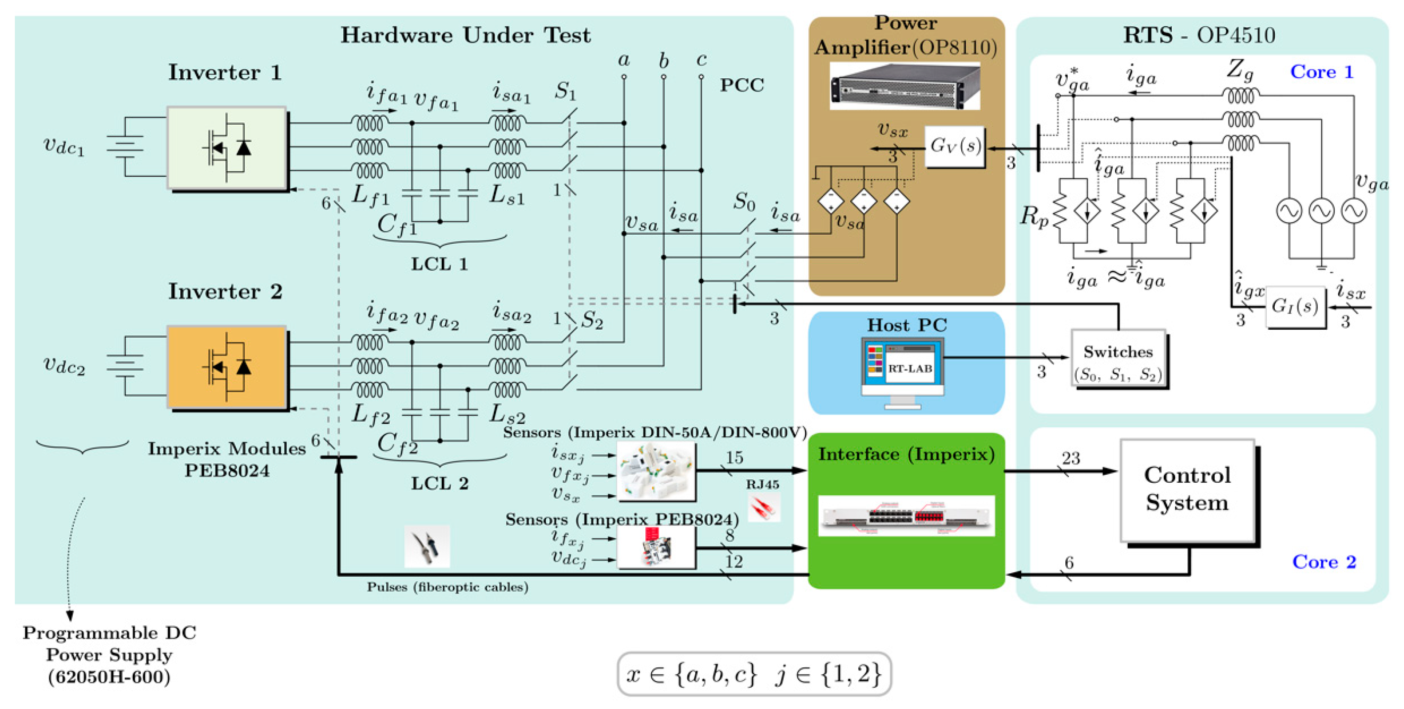
• To enhance this stage, the previous simulation steps were needed to tune the device regarding the interphase model, filters, and delays to improve this stage. Although it seems trivial, it is not; the power amplifier’s safety, the result’s quality, and the capability to disseminate reliable results are highly dependent on it. That is why it is highly recommended that the interconnection model be recorded in all the PHIL articles.
• Figure 7 shows multiple current and voltage sensors, and depending on the application, different sensed variables can interact with the simulation. Before any attempt at simulation, a meticulous sensor calibration process should be performed to ensure that the correct scaling has been used and the offsets have been eliminated to communicate the actual variables with the simulation.
• The power amplifier (OP8110 in this case) is the decisive device that empowers the PHIL simulation. From a practical standpoint, it permits bidirectional power flow between the HUT and the amplifier, considering any equivalent circuit model in the software. From the scientific viewpoint, the impact is much broader. Figure 7 shows a conceptualization of a microgrid with inverters that can operate in the grid forming or grid following mode for different purposes. Nevertheless, the simulation conceptualization can be of any other level of complexity. For instance, it can include the operation of protection devices, applications of distributed generation, virtual inertia converters, studies of controller schemes or hierarchical control of distributed energy resources, battery energy storage systems integrated into the facility, power systems analysis, smart-grid concepts, electric vehicles, communication protocols, and the developments of cyber-attack defense and a significant possibility of topics.
• The RTS-OP4510 device is the most elaborated expression of science, where researchers can develop their ideas, hypotheses, and experimentation to obtain high-quality results. Nevertheless, for this purpose, it is necessary to consider the following:
• The equivalent circuit interconnecting to the amplifier is programmed into the RTS-OP4510. Observe, from Figure 7 that the sensed currents $i_{sx}$ are the inputs of the transfer function $G_I\left(s\right)={\displaystyle \frac{1}{T_{fb}s+1}}$, where $T_{fb}={\displaystyle \frac{1}{2\pi f_{fb}}}$ and $f_{fb}$ is the bandwidth of the feedback filter. The output of the filter are the currents ${\widehat{i}}_{gx}$. As was said in the previous stage, the filter polynomial order and cut-off frequency are critical for the simulation stability and, consequently, for the amplifier safety.
• Also, Figure 7 shows that at the point of common coupling with the power amplifier, another transfer function $G_V\left(s\right)={\displaystyle \frac{1}{T_{bw}s+1}}{\mathrm{e}}^{s\left(T_{\mathrm{rts}}+T_{\mathrm{OP}8110}\right)}$ $T_{bw}={\displaystyle \frac{1}{2\pi f_{bw}}},f_{bw}=10 \mathrm{kHz}$, T_rts = 20 μs, is the time step of the real-time simulation. Selecting this time step depends on the computational capability. Of course, having a reduced time step is convenient, but then overruns are more likely. Therefore, the programmer should be efficient in their programming process. Therefore, the efficacy of the simulation is a parameter to be considered. An intrinsic delay of the power amplifier OP8110 is T_OP8110 = 8 μs.
• A great versatility is that users can leverage the cores of the RTS-OP4510 to organize resources better. In this case, the control system, where the control law is calculated, is hosted in a different core for better processing. The PWM switches control signals are interfaced through the inverters by an IMPERIX interface, as seen in Figure 7.
• There are several possibilities to calibrate and minimize the measurement errors of each sensor. As a suggestion, the user can program an FFT algorithm to decouple the DC from the AC part of the signals. Take a known signal from a controlled source and pass it across the sensor. In this way, the user can calibrate the offset and scale with the correct gains to ensure the proper value of the signals.

Before leaving the green-dotted line block of Figure 1, observe the inclusion of a block related to model interconnection research. This block represents an excellent opportunity to do deep research oriented to enhance the quality of possible scenarios to put under test, as some articles have shown [36,37,38]. When the HUT and the equivalent circuit to be programmed on the software side have high complexity, the previously explained bullets are likely insufficient. In that case, running analysis and algorithms to identify the equivalent circuit of the plant to analytically explore the stability region of the interconnection regarding the HUT operation can be required. Additionally, proposing and tuning closed-loop controllers for the interconnection algorithm is a fertile field of research to be explored. At the end of the flow diagram proposed in Figure 1, what results is a record of the PHIL simulation, obtaining all the possible information and results to enhance the research.

Figure 8 shows a photograph of the PHIL platform of simulation.

From Figure 8, the elements that constitute the PHIL simulation based on OPAL-RT can be seen. From the left to the right, the first element that can be seen is the power inverters. They are two three-phase inverters IMPERIX-based modules PEB8024, 1200 V, 36 A SiC MOSFETS. Following to the right, it can be observed the local loads are resistances used for heating with a capability of 1 kW at 120 V. The following elements are the LCL filters. A combination of magnetic and air cores for the inductors can be observed. This is because the magnetic core being available during the experiments was limited. The capacitors used were based on polypropylene 400 V. After that, the current DIN 50 IMPERIX (±50 A) and DIN 800 IMPERIX (±800 V) sensors are indicated using orange letters. Finally, the OPAL-RT device is connected to the hardware using red ethernet cables, which can be seen on the right.

Figure 9 shows a template used to connect the hardware and software to perform the PHIL simulation.

The blocks of Figure 9 are numbered according to their purpose as follows:

1. Inputs: The block OpComm receives all the measured signals required in the experiment.

2. Grid: This block contains three main blocks.

(a) Impedance, in that the block is programmed with a switch that changes the impedance of the modeled grid, considering a zero logic for a weak equivalent impedance (low short circuit capability) and one logic for a stiff equivalent impedance (higher short circuit capability).

(b) Interface Algorithm, in that block, is programmed as the model interface between the hardware under test and the model programmed into the OP4510. Also, in this sub-block, the filters required for providing stability are tuned and programmed. This is an interesting research gap where multiple groups are developing work [29,31,39,40] to improve the interface performance, extend the possible scenarios to be simulated, and guarantee better care of the power amplifiers.

(c) The OP8110 Interface Group Communication Block is intrinsic to the power amplifier provided by the OPAL-RT supplier. In this case, the power amplifier is built using switching-mode power supplies, but linear amplifiers and several power capabilities are also available.

3. Switches S0, S1, and S2: In this block, the label OpOutput provides the switches with information on the amplitude modulation index (ma) and switching frequency.

4. PLLs: In this block, there are two PLLs. The electrical angle can be obtained directly from power amplifier measurements v_gx (x ∊ {a, b, c}) or the voltages v_sx at the PCC. This offers additional flexibility for testing different control structures. The “OpInput” communication block receives signals from the input/output interface. In this case, the analog voltage outputs at the PCC are collected using the DIN-800V devices and the IMPERIX interface, and then passed to the OP4510 input/output interface through a DB37 connector.

5. Secondary control: This is an interesting block because it can develop the complete controller scheme concept for the different operation modes of the inverters, such as grid forming or grid following.

To illustrate the flexibility of the real-time PHIL simulation, consider the scopes shown in Figure 10, Figure 11, Figure 12 and Figure 13.

The scopes show some selected results for illustrating the several capabilities of obtaining scenarios. In this case, all the PHIL simulated scenarios are carried out using the inverters in the grid-following mode.

Figure 10 shows a steady-state result where inverter one contributes 12.25 VAR. In contrast, inverter two contributes 81.65 W. Figure 11 shows a decoupled transient state where only inverter one experiments with an active power step from 0 W to 45.19 W while the reactive power is maintained at 0 VAR. Inverter two is kept in a steady state with the active power at 117.8 W while the reactive power is at 0 VAR. Figure 12 and Figure 13 show the capability of contributing with apparent power. In Figure 12, inverter one contributes with a lead current (more capacitive), while inverter two has a lag current (more inductive). Figure 13 shows both inverters contributing to lag current (more inductive).

Lessons Learned of Power-Hardware-in-the-Loop Simulation

As can be seen in Figure 7, the converter controller is programmed in the second core of the RTS-OP4510. However, that controller can also be programmed in an external setup, exchanging signals with the simulation. Why did I not do that? The project scope was the same. Nevertheless, it is relevant to say that in terms of an actual application, industrial, for instance, the possibility of programming the controller using an actual industrial device increases tremendously the possibility of guaranteeing the success of implementing a concept in an actual application.

Table 4. Merits and drawbacks of stage 4.

Merits
PHIL simulation is the most realistic scenario, very near to an actual application. Grid equivalent circuits can be changed dynamically or can be modified according to specific requirements. HUT control schemes face more realistic circumstances. It opens ways for improving systems, but even better, to identify new challenges or research gaps.
Drawbacks
It requires very sophisticated training and time. It requires a skilled professional person dedicated entirely to manipulating the equipment. It is expensive equipment; therefore, the insurance and maintenance cost is expensive.

summarizes the merits and drawbacks of this stage as the authors conceptualized them.

4. Conclusions

PHIL simulation should be considered an influential way to reach the relevant research results. The research gap to be addressed should be established, the methodologies or possible new theories to be used identified, and the required work to advance from a conceptualized idea to formulate a clear scope of the research, respecting the scientific method, should be clear. Once the previous steps have been taken, taking advantage of the PHIL simulation concept will be more natural.

However, given the equipment described in Figure 7, the fundamental question is as follows: Is it only a powerful tool? Or does it empower scientific research?

After completing the learning curve for PHIL simulation in OPAL-RT, the findings have been multiple, varied, and enriching, which gave rise to this article, whose profile aims to be reflective but valuable for those who begin this learning curve.

In the initial stages, when a model is conceptualized for which a real-time PHIL simulation is to be performed, the results and conclusions that can be obtained from offline simulations and real-time model-in-the-loop (MIL) simulations are the same. It is common to ask the following question: What new knowledge do real-time MIL simulations provide? Why do real-time MIL simulations on expensive equipment such as OPAL-RT or RTDS? MIL simulation is the same approach as offline model simulation. Still, it provides the quality of programming the simulator with the requirements to eventually replace mathematical approximations with actual elements. Programming simulations with a fixed step and deciding on the constant integration step may seem trivial. Formulating a simulation that includes interconnection models, sensor delays, and the power amplifier transfer function, which also transmits and receives signals outside, can help the novice user better understand his simulator and avoid putting the amplifier’s safety at risk as much as possible.

The main merit that we have wanted to highlight with the flow chart is that the researcher, through a series of documented steps, can achieve a replacement of mathematical models with real plants, as in the case of the inverters presented in this article, and thus interact, in a flexible way, with network models that may not be available in a laboratory. This enriches the possibilities of carrying out applied research with an industrial approach in a safer way and with lower investment requirements in prototypes.

However, the flexibility required has an issue that is currently being investigated. That is, the integration of hardware into the simulation to interact with a complex network model, for example, where there is renewable and conventional energy, requires interconnection algorithms that guarantee the simulation stability and the amplifier safety. There are, therefore, efforts to approach interconnection algorithms from the perspective of automatic control and thus provide the system with more significant operating margins when faced with equivalent models or more extensive hardware requirements. This allows the conclusion that real-time simulation equipment should not be seen only as a tool for testing systems but as a beneficial scientific concept for taking mathematical conceptualizations to the field of formulations with actual equipment and thereby testing, with better results, advanced ideas of applied science. This article is intended to be a helpful guide that helps to ask the right questions in building a PHIL simulation. The correct answers will depend on the equipment type and the scope of the simulations to be carried out.

References

1. Ulerio, R.O.S.; Nowocin, J.K.; Smith, C.L.; Rekha, R.P.; Corbett, E.G.; Limpaecher, E.R.; LaPenta, J.M. Development of a Real-Time Hardware-in-the-Loop Power Systems Simulation Platform to Evaluate Commercial Microgrid Controllers. Technical Report. Available online: https://www.ll.mit.edu/sites/default/files/publication/doc/development-real-time-hardware-in-the-loop-power-systems-salcedo-ulerio-tr-1203.pdf (accessed on 4 November 2024).
2. García-Martínez, E.; Sanz, J.F.; Muñoz-Cruzado, J.; Perié, J.M. A Review of PHIL Testing for Smart Grids—Selection Guide, Classification and Online Database Analysis. Electronics 2020, 9, 382. [Google Scholar] [CrossRef]
3. Rathnayake, D.B.; Akrami, M.; Phurailatpam, C.; Me, S.P.; Hadavi, S.; Jayasinghe, G.; Zabihi, S.; Bahrani, B. Grid Forming Inverter Modeling, Control, and Applications. IEEE Access 2021, 9, 114781–114807. [Google Scholar] [CrossRef]
4. Kotsampopoulos, P.; Georgilakis, P.; Lagos, D.T.; Kleftakis, V.; Hatziargyriou, N. FACTS Providing Grid Services: Applications and Testing. Energies 2019, 12, 2554. [Google Scholar] [CrossRef]
5. Simões, M.G.; Ribeiro, P.F. Education in Electrification for Societal Sustainability: History and philosophy. IEEE Electrific. Mag. 2024, 12, 89–99. [Google Scholar] [CrossRef]
6. Simões, M.G. The Evolution of Electrification—From a Non-Plan Toward an Engineering Achievement—Early Years [History]. IEEE Electrific. Mag. 2024, 12, 92–96. [Google Scholar] [CrossRef]
7. Ghosh, A.; Zare, F. Control of Power Electronic Converters with Microgrid Applications; Wiley: Hoboken, NJ, USA, 2023; ISBN 978-1-119-81546-4. [Google Scholar]
8. Ismail, M.A.; Alfouly, A.; Hussein, H.S.; Hamdan, I. Hardware in the Loop Real-Time Simulation of Improving Hosting Capacity in Photovoltaic Systems Distribution Grid With Passive Filtering Using OPAL-RT. IEEE Access 2023, 11, 78119–78134. [Google Scholar] [CrossRef]
9. Sidorov, V.; Chub, A.; Vinnikov, D.; Lindvest, A. Novel Universal Power Electronic Interface for Integration of PV Modules and Battery Energy Storages in Residential DC Microgrids. IEEE Access 2023, 11, 30845–30858. [Google Scholar] [CrossRef]
10. Jain, R.; Sawant, J.R.; Pratt, A. A Power-Hardware-in-the-Loop (PHIL) Evaluation of Service Restoration With Networked Microgrids. In Proceedings of the 2024 IEEE Power & Energy Society General Meeting (PESGM), Seattle, WA, USA, 21–25 July 2024. [Google Scholar] [CrossRef]
11. Kikusato, H.; Ustun, T.S.; Suzuki, M.; Sugahara, S.; Hashimoto, J.; Otani, K.; Shirakawa, K.; Yabuki, R.; Watanabe, K.; Shimizu, T. Microgrid Controller Testing Using Power Hardware-in-the-Loop. Energies 2020, 13, 2044. [Google Scholar] [CrossRef]
12. Alzate-Drada, S.; Montano-Martinez, K.; Andrade, F. Energy Management System for a Residential Microgrid in a Power Hardware-in-the-Loop Platform. In Proceedings of the 2019 IEEE Power & Energy Society General Meeting (PESGM), Atlanta, GA, USA, 4–8 August 2019; pp. 1–5. [Google Scholar] [CrossRef]
13. Ceceña, A.A. Power Hardware-in-the-Loop Interfacing of Grid-Forming Inverter for Microgrid Islanding Studies. In Proceedings of the 2023 IEEE Power & Energy Society Innovative Smart Grid Technologies Conference (ISGT), Washington, DC, USA, 16–19 January 2023; pp. 1–5. [Google Scholar] [CrossRef]
14. Pratt, A.; Prabakar, K.; Ganguly, S.; Tiwari, S. Power-Hardware-in-the-Loop Interfaces for Inverter-Based Microgrid Experiments Including Transitions. In Proceedings of the 2023 IEEE Energy Conversion Congress and Exposition (ECCE), Nashville, TN, USA, 29 October–2 November 2023; pp. 537–544. [Google Scholar] [CrossRef]
15. Ren, W. Accuracy Evalaution of Power Hardware-in-the-Loop (PHIL) Simulation. Available online: https://www.proquest.com/openview/effd1ea0813a34dde56f0030feff5221/1?pq-origsite=gscholar&cbl=18750 (accessed on 24 October 2024).
16. Kothandaraman, S.R.; Malekpour, A.; Maigha, M.; Paaso, A.; Zamani, A.; Katiraei, A. Utility Scale Microgrid Controller Power Hardware-in-the-Loop Testing. In Proceedings of the IEEE Electronic Power Grid (eGrid), Charleston, SC, USA, 12–14 November 2018; IEEE: Piscataway, NJ, USA; pp. 1–6. [Google Scholar] [CrossRef]
17. Samano-Ortega, V.; Rodriguez-Estrada, H.; Rodríguez-Segura, E.; Padilla-Medina, J.; Aguilera-Alvarez, J.; Martinez-Nolasco, J. Power Sharing Control in a Grid-Tied DC Microgrid: Controller Hardware in the Loop Validation. Appl. Sci. 2021, 11, 9295. [Google Scholar] [CrossRef]
18. Vodyakho, O.; Edrington, C.S.; Steurer, M.; Azongha, S.; Fleming, F. Synchronization of three-phase converters and virtual microgrid implementation utilizing the Power-Hardware-in-the-Loop concept. In Proceedings of the 2010 Twenty-Fifth Annual IEEE Applied Power Electronics Conference and Exposition (APEC), Palm Springs, CA, USA, 21–25 February 2010; pp. 216–222. [Google Scholar] [CrossRef]
19. Nasab, M.R.; Cometa, R.; Bruno, S.; Giannoccaro, G.; Scala, M.L. Power Systems Simulation and Analysis: A Review on Current Applications and Future Trends in DRTS of Grid-Connected Technologies. IEEE Access 2024, 12, 121320–121345. [Google Scholar] [CrossRef]
20. Dow, A.R.R.; Darbali-Zamora, R.; Flicker, J.D.; Palacios, F.; Csank, J.T. Development of Hierarchical Control for a Lunar Habitat DC Microgrid Model Using Power Hardware-in-the-Loop. In Proceedings of the 2022 IEEE 49th Photovoltaics Specialists Conference (PVSC), Philadelphia, PA, USA, 5–10 June 2022; pp. 0754–0760. [Google Scholar] [CrossRef]
21. Colet-Subirachs, A.; Paradell, P.; Vasquez, J.L.; Dominguez-Garcia, J.L.; Pampliega, D.; Ramos, F.; Gallart-Fernandez, R. Cyberattack Mitigation in a Microgrid Environment: A Power-Hardware-in-The-Loop testing methodology. In Proceedings of the 2022 IEEE International Conference on Environment and Electrical Engineering and 2022 IEEE Industrial and Commercial Power Systems Europe (EEEIC/I&CPS Europe), Prague, Czech Republic, 28 June 2022–1 July 2022; pp. 1–6. [Google Scholar] [CrossRef]
22. Kasper, L.; Schwarzmayr, P.; Birkelbach, F.; Javernik, F.; Schwaiger, M.; Hofmann, R. A digital twin-based adaptive optimization approach applied to waste heat recovery in green steel production: Development and experimental investigation. Appl. Energy 2024, 353, 122192. [Google Scholar] [CrossRef]
23. Glass, P.; Di Marzo Serugendo, G. Coordination Model and Digital Twins for Managing Energy Consumption and Production in a Smart Grid. Energies 2023, 16, 7629. [Google Scholar] [CrossRef]
24. Shitole, A.B.; Kandasamy, N.K.; Liew, L.S.; Sim, L.; Bui, A.K. Real-Time Digital Twin of Residential Energy Storage System for Cyber-Security Study. In Proceedings of the 2021 IEEE 2nd International Conference on Smart Technologies for Power, Energy and Control (STPEC), Bilaspur, Chhattisgarh, India, 19–22 December 2021; pp. 1–6. [Google Scholar] [CrossRef]
25. Testasecca, T.; Lazzaro, M.; Sirchia, A. Towards Digital Twins of buildings and smart energy networks: Current and future trends. In Proceedings of the 2023 IEEE International Workshop on Metrology for Living Environment (MetroLivEnv), Milano, Italy, 29–31 May 2023; pp. 96–101. [Google Scholar] [CrossRef]
26. Sayed-Mouchaweh, M. (Ed.) Artificial Intelligence Techniques for a Scalable Energy Transition: Advanced Methods, Digital Technologies, Decision Support Tools, and Applications; Springer International Publishing: Cham, Switzerland, 2020; ISBN 978-3-030-42725-2. [Google Scholar] [CrossRef]
27. Szcześniak, P.; Grobelna, I.; Novak, M.; Nyman, U. Overview of Control Algorithm Verification Methods in Power Electronics Systems. Energies 2021, 14, 4360. [Google Scholar] [CrossRef]
28. Hoang, T.T.; Nair, N.-K.C. Advanced Approach for Stability Assessment of PHIL Setups Coupled by Clarke-Park Transform. In Proceedings of the 2023 IEEE Power & Energy Society General Meeting (PESGM), Orlando, FL, USA, 16–20 July 2023; pp. 1–5. [Google Scholar] [CrossRef]
29. Lundstrom, B.; Salapaka, M.V. Optimal Power Hardware-in-the-Loop Interfacing: Applying Modern Control for Design and Verification of High-Accuracy Interfaces. IEEE Trans. Ind. Electron. 2021, 68, 10388–10399. [Google Scholar] [CrossRef]
30. Upamanyu, K.; Narayanan, G. Improved Accuracy, Modeling, and Stability Analysis of Power-Hardware-in-Loop Simulation With Open-Loop Inverter as Power Amplifier. IEEE Trans. Ind. Electron. 2020, 67, 369–378. [Google Scholar] [CrossRef]
31. Constantine, J.; Lian, K.L.; Yang, N.-T. A New Interface for Power Hardware-in-the-Loop Simulation Using Nelder–Mead Algorithm Une nouvelle interface pour la simulation Hardware-in-the-Loop de puissance à l’aide de l’algorithme de Nelder-Mead. IEEE Can. J. Electr. Comput. Eng. 2025, 48, 10–18. [Google Scholar] [CrossRef]
32. Ruiz, Y.L.; Ramirez, J.S.; Nuñez, C.; Visairo, N. Preliminary Power Hardware in the Loop Simulation of a Microgrid Test Bench in OPAL-RT. In Proceedings of the CONCAPAN XLII, San José, Costa Rica, 27–29 November 2024. [Google Scholar]
33. Ojaghloo, B.; Gharehpetian, G.B. Power Hardware In The Loop Realization, Control and Simulation. Renew. Energy Power Qual. J. 2017, 1, 108–113. [Google Scholar] [CrossRef]
34. Tozak, M.; Taskin, S.; Sengor, I.; Hayes, B.P. Modeling and Control of Grid Forming Converters: A Systematic Review. IEEE Access 2024, 12, 107818–107843. [Google Scholar] [CrossRef]
35. Hatakeyama, T.; Riccobono, A.; Monti, A. Stability and accuracy analysis of power hardware in the loop system with different interface algorithms. In Proceedings of the 2016 IEEE 17th Workshop on Control and Modeling for Power Electronics (COMPEL), Trondheim, Norway, 27–30 June 2016; pp. 1–8. [Google Scholar] [CrossRef]
36. Lauss, G.; Strunz, K. Accurate and Stable Hardware-in-the-Loop (HIL) Real-Time Simulation of Integrated Power Electronics and Power Systems. IEEE Trans. Power Electron. 2021, 36, 10920–10932. [Google Scholar] [CrossRef]
37. Bigarelli, L.; di Benedetto, M.; Lidozzi, A.; Solero, L. Stability and Accuracy Evaluation of LCL Coupling Networks for PMSM Emulation PHIL. In Proceedings of the IEEE Energy Conversion Congress and Exposition (ECCE), Detroit, MI, USA, 9–13 October 2022; IEEE: Piscataway, NJ, USA; pp. 1–7. [Google Scholar] [CrossRef]
38. Ayasun, S.; Fischl, R.; Vallieu, S.; Braun, J.; Çadırlı, D. Modeling and stability analysis of a simulation–stimulation interface for hardware-in-the-loop applications. Simul. Model. Pract. Theory 2007, 15, 734–746. [Google Scholar] [CrossRef]
39. Rimorov, D.; Forbes, J.R.; Tremblay, O.; Gagnon, R. Robust Impedance Emulation for Transmission Line Interface in Power-Hardware-In-the-Loop Applications: Optimal Filter Approach. IEEE Open J. Ind. Electron. Soc. 2025, 6, 158–169. [Google Scholar] [CrossRef]
40. Hernandez-Alvidrez, J.; Darbali-Zamora, R.; Flicker, J.D.; Gurule, N.S. Testing Functional Capabilities of Commercial Grid Forming Inverters Using a Power Hardware-in-the-Loop Setup. In Proceedings of the 2024 IEEE 52nd Photovoltaic Specialist Conference (PVSC), Seattle, WA, USA, 9–14 June 2024; pp. 0759–0765. [Google Scholar] [CrossRef]
Figure 1. Flow diagram of the proposed process for PHIL simulation.
Inventions 10 00019 g001
Figure 2. Microgrid scheme used as an object of study.
Inventions 10 00019 g002
Figure 3. The general structure of the real-time simulation.
Inventions 10 00019 g003
Figure 4. The inverter circuit of the real-time simulation.
Inventions 10 00019 g004
Figure 5. Ideal transformer interconnection model.
Inventions 10 00019 g005
Figure 6. Simulation template of one inverter.
Inventions 10 00019 g006
Figure 7. PHIL simulation of the AC microgrid under study.
Inventions 10 00019 g007
Figure 8. A photograph of the microgrid PHIL simulation based on the OPAL-RT.
Inventions 10 00019 g008
Figure 9. PHIL simulation template using OPAL-RT.
Inventions 10 00019 g009
Figure 10. Steady state. Inverter 1: P = 0 W, Q = 12.25 VAR; inverter 2: P = 81.65 W, Q = 0 VAR.
Inventions 10 00019 g010
Figure 11. Transient state. Inverter 1: P from 0 W to 45.19 W, Q = 0 VAR. Steady state. Inverter 2: P = 117.8 W, Q = 0 VAR.
Inventions 10 00019 g011
Figure 12. Steady State. Inverter 1: S = 141.60 VA more capacitive current. Inverter 2: S = 265.19 VA more inductive current.
Inventions 10 00019 g012
Figure 13. Steady State. Inverter 1: S = 155.60 VA. Inverter 2: S = 181.35 VA. Inverter 2: S = 265.19 VA. Both inverters with more inductive currents.
Inventions 10 00019 g013