Abstract
Predictive maintenance in industrial machinery relies on the timely detection of component faults to prevent costly downtime. Rolling bearings, being critical elements, are particularly prone to defects such as outer race faults and ball spin defects, which manifest as characteristic vibration patterns. In this study, we introduce a novel bearing vibration dataset collected on a testbench under both constant and variable rotational speeds (0–5000 rpm), encompassing healthy and faulty conditions. The dataset was used for failure classification and further enriched through feature engineering, resulting in input features that include raw acceleration, signal envelopes, and time- and frequency-domain statistical descriptors, which capture fault-specific signatures. To quantify prediction uncertainty, two different approaches are applied, providing confidence measures alongside model outputs. Our results demonstrate the progressive improvement of classification accuracy from 87.2% using only raw acceleration data to 99.3% with a CNN-BiLSTM (Convolutional Neural Network–Bidirectional Long Short-Term Memory) ensemble and advanced features. Shapley Additive Explanation (SHAP)-based explainability further validates the relevance of frequency-domain features for distinguishing fault types. The proposed methodology offers a robust and interpretable framework for industrial fault diagnosis, capable of handling both stationary and non-stationary operating conditions.
1. Introduction
Modern industrial machinery is increasingly complex, necessitating proactive strategies to ensure reliability and minimize downtime. Predictive maintenance has emerged as a key solution that exploits sensor data and Machine Learning (ML) models, enabling early detection of potential faults. Consequently, it reduces unplanned downtime and optimizes maintenance schedules, extending the operational lifespan of equipment while reducing costs [1].
Recent advances in ML have significantly improved Fault Diagnosis and Prognosis (FDP) [2]. By analyzing large volumes of sensor data, ML algorithms can detect patterns and anomalies indicative of component failures. This allows for both real-time detection and predictive insights, supporting optimized maintenance schedules and improved overall machine reliability.
Among critical components, rolling bearings are particularly prone to faults such as wear, misalignment, and ball defects [3]. Failure of these elements can propagate severe damage throughout machinery, making real-time monitoring essential [4]. Vibration signals, temperature fluctuations, and other performance indicators provide rich information for assessing bearing health, detecting early-stage faults, and informing timely maintenance decisions.
This work is an extension of the paper “A Novel Benchmark for Fault Detection in Rolling Bearings Using CNNs and Monte Carlo Dropout” [5]. Building upon the dataset introduced in the conference paper, we develop a classification framework based on different neural network architectures with white-box feature selection informed by domain knowledge to operate both in constant and variable speed conditions. Features include raw accelerations, envelopes, and statistical and spectral descriptors. To increase trust in predictions, Monte Carlo (MC) dropout is applied for uncertainty quantification.
The remainder of this paper is structured as follows: Section 2 describes the problem and the challenges of bearing fault detection. Section 3 details the experimental setup, dataset creation, feature extraction, and model architectures. Section 4 presents classification results, model comparisons, and explainability analyses. Finally, Section 5 concludes the study and outlines directions for future research.
2. Problem Description
Bearings are critical components in many industrial machines, experiencing wear and tear throughout their operational life. Over time, this wear can result in increased vibrations, causing different faults, and finally leading to failures and costly downtime [6]. To prevent these scenarios, the health of the bearings must be continuously monitored using sensors, i.e., accelerometers, in order to analyze real-time acceleration data. This, combined with a proactive maintenance approach, could lead to early identification of failures, allowing for programmed interventions to prevent more severe damage.
2.1. Physical Mechanisms of Rolling Bearing Faults
Rolling element bearings are composed of an inner race, an outer race, rolling elements (balls or rollers), and a cage. Localized defects typically initiate as pits or spalls on one of these elements and, as each rolling element passes over the damaged zone [7]. These defects produce distinct vibration signatures, which are determined by the kinematics of the rolling elements and the spatial relationship between the defect and the load zone. For faults located on the outer race, the damage remains stationary relative to the radial load, resulting in each rolling element generating an impact of similar amplitude as it traverses the defect. This process produces a nearly periodic train of impulses at the Ball Pass Frequency Outer Race (BPFO), with its harmonic series clearly observable in both the vibration envelope and the demodulated spectrum. In contrast, defects on rolling elements generate a different signature. Here, the defect rotates with the ball and enters the load region only intermittently, leading to amplitude-modulated bursts centered at the Ball Spin Frequency (BSF) with characteristic sidebands at the Fundamental Train Frequency (FTF). Inner-race defects display hybrid characteristics, producing impulses at the Ball Pass Frequency Inner Race (BPFI) as the rotating defect aligns with the load direction once per shaft revolution. These defects also induce shaft-speed sidebands due to periodic variations in the dynamic transfer path [8,9]. These classical analytical bearing models, when combined with modern cyclostationary-based interpretations, account for periodic impulses, modulation sidebands, and resonance-rich transients in measured vibration signals [7,10,11]. Consequently, such physics-based understanding underpins the diagnostic interpretation and feature design utilized in the present study.
2.2. Signal Characteristics and Feature Foundations for Fault Diagnosis
Low computing burden and straightforward interpretability make time- and frequency-domain indicators essential for rolling–bearing condition monitoring. The Root Mean Square (RMS) metric is widely used as an energy-based severity indicator for time, which becomes more excited by fault-induced impacts. This behavior is consistently studied in both industrial and controlled degradation studies. Higher-order statistics, such as kurtosis, skewness, and crest factors, have also demonstrated strong effectiveness in identifying early-stage localized defects [12]. However, in multiscale fault-severity analyses, alternative metrics such as the Energy Index (EI), which compare segmental and global RMS levels, have been suggested due to the known non-monotonicity of kurtosis at advanced deterioration stages [13]. Frequency-domain analysis, however, provides a direct mapping between bearing kinematics and spectral content, enabling the identification of characteristic fault frequencies together with their modulation-induced sidebands. Spectral decomposition, which is performed using band-pass filtering, Hilbert transform demodulation, and decomposition, extracts low-frequency fault signatures embedded within excited higher-frequency resonances [14,15]. In addition to introducing adaptive demodulation band selection, Hilbert–Huang–based demodulation, and cyclostationary estimators have advanced the extraction of repetitive transient patterns under realistic industrial operation [16].
The analysis of bearing data and detection of possible faults is a time-dependent challenge, consisting of a time series classification problem. In recent years, ML and Deep Learning (DL) methods have been increasingly applied to tackle this challenge [5,17]. These techniques have proven to be effective in extracting meaningful patterns from complex vibration data, offering a powerful tool for fault diagnosis.
A wide range of methodologies has been developed over the past decade to address bearing fault detection, starting from more traditional machine learning techniques based on decision trees [18,19], support vector machines (SVMs) [20,21] and K-Nearest Neighbors (KNN) [22,23], to more recent methods, in the DL area, like CNNs [24,25], LSTMs [26,27], and Recurrent Neural Networks (RNNs) [28] to improve diagnostic accuracy and robustness. The main characteristics and results of these studies are summarized in Table 1.

Table 1.
State-of-the-art in bearing fault classification.
In this study, we also propose using MC Dropout [35] to estimate uncertainty in deep learning model predictions, building on techniques commonly used in explainable AI [36], to better understand the reliability of the model’s predictions. MC Dropout is a form of approximate Bayesian inference that enables uncertainty estimation during the inference phase by applying dropout at test time, which is typically only used during training.
In standard neural networks, dropout randomly disables a fraction of neurons during training to prevent overfitting. However, by applying dropout during testing, the model effectively generates a distribution of predictions, allowing us to quantify uncertainty. Specifically, by performing multiple stochastic forward passes with dropout, we can approximate the predictive distribution and estimate the uncertainty in the model’s predictions.
The main idea behind MC Dropout, as shown in Figure 1a is that by performing multiple forward passes with different dropout masks, we can treat these different predictions as samples from the posterior distribution of the model. This allows the model to not only output predictions, but also provide a measure of confidence.
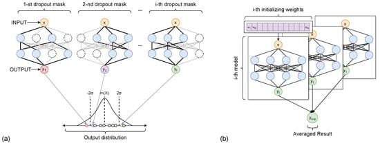
Figure 1.
Uncertainty quantification methods. (a) Monte Carlo Dropout: x is the given input, and are the outputs generated by applying n different dropout masks that form the final distribution. (b) Deep Ensemble: multiple models are independently trained with different initializations and combined at inference. The diversity among models enables improved accuracy and uncertainty estimation.
Ensemble learning [37] represents another widely used approach for estimating predictive uncertainty in deep learning models, commonly referred to as Deep Ensembles. Unlike MC Dropout, which relies on stochastic forward passes of a single neural network, Deep Ensembles employ multiple independently trained models, each initialized with different random weights and often trained using shuffled subsets of the training data [38]. The diversity among ensemble members arises from variations in initialization and training dynamics, which lead the models to converge to different local minima in the loss landscape. A graphical representation of this process is shown in Figure 1b.
Each model within the ensemble is typically trained using standard loss functions, such as Mean Squared Error (MSE) for regression tasks or Categorical Cross-Entropy for classification, without explicitly modeling uncertainty during training. In this standard setup, uncertainty estimation emerges naturally during inference, where the predictions of all ensemble members are aggregated, commonly by averaging their output probabilities, to obtain the final prediction. The variance among the individual model outputs reflects the epistemic uncertainty of the model: if all models yield similar predictions, the variance is low, indicating high confidence; conversely, large disagreement among models corresponds to higher uncertainty.
In more advanced formulations, probabilistic loss functions (e.g., those based on likelihood maximization or Bayesian principles) can be employed during training to capture not only epistemic but also aleatoric uncertainty—that is, uncertainty inherent in the data itself. However, such probabilistic training remains an extension beyond the standard Deep Ensemble framework.
3. Methodology
3.1. Experimental Setup
To create the dataset that we used in this paper, we used the ISE OneX Test Bench, shown in Figure 2a, which is a platform designed for simulating and evaluating the performance of rotating machines under different conditions, such as imbalances or defective components. The test bench includes a Siemens brushless AC motor powered by a 230 V, 50/60 Hz supply with a maximum current of 3 A. The motor’s nominal power is 0.2 kW, with a standard speed of 3000 rpm and a maximum speed of 5000 rpm. Its nominal torque is 0.64 Nm (maximum 1.91 Nm), with three replaceable rolling bearings, identified (by the arrows) as 1,2,3 in Figure 2b, and two discs integral with the rotation axis. The test bench operates within a temperature range of +5 °C to +40 °C and can handle humidity levels up to 50% at +40 °C. For monitoring purposes, it is equipped with various sensors to track and analyze the machine’s behaviors and performance degradation under various malfunctioning conditions.
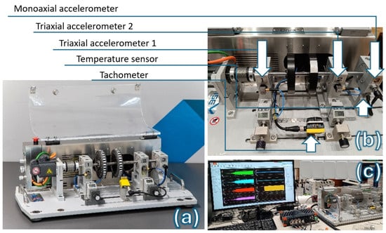
Figure 2.
ISE OneX test-bench platform for evaluating the performance of rotating machines under different conditions (a). Integrated sensors with OneX test bench for monitoring (b). Experimental setup to measure the vibration using healthy and faulty bearings using 8-channel SIRIUSi data acquisition system (c).
As shown in Figure 2b, the test bench is equipped with different sensors. For vibration analysis, the bench includes two triaxial accelerometers manufactured by PCB PIEZOELECTRONICS placed on the bearings housing (1 and 2). These accelerometers have a sensitivity of 100 mV/g and are capable of detecting vibrations in all three axes. Additionally, an axial sensor from PCB PIEZOELECTRONICS with a sensitivity of 100 mV/g is used on bearing 3 for further vibration analysis. A retroreflective mode tachometer from Banner Engineering is used to monitor the speed of the rotating motor axis, providing precise speed control with a resolution of 1 rpm. A temperature sensor is placed on bearing 3 to measure temperature variations, with an accuracy of ±0.1 °C.
The test bench includes several test functionalities to simulate different mechanical issues and assess the system’s response under various fault conditions. Imbalance simulation is achieved by adding or removing weights from the test bench’s rotating disks, allowing for a test of the system’s reaction to static and dynamic imbalances. Bearing wear is simulated by replacing healthy bearings with faulty bearings, enabling the analysis of system behavior when components are worn. The test bench also allows for the simulation of loose machine structures by adjusting its feet, which helps study the impact of loose components on performance. Additionally, both horizontal and vertical misalignments can be simulated by adjusting the positioning of the motor and bearings, enabling the evaluation of how misalignment affects machine operation. Figure 2c shows our experimental setup used to measure the vibration using healthy and faulty bearings. An 8-channel SIRIUSi data acquisition system, manufactured by DEWEsoft® (Trbovlje, Slovenia), is utilized to acquire signals. With the introduction of native integrated electronic piezoelectric (IEPE) mode, the module supports DC or AC mode input coupling with 0.16 Hz high-pass filter for low ranges (0.3 Hz for 100 V range). It features a dual 24-bit Delta-sigma ADC with a sampling rate of 200 kS/s for each channel. A summary of the sensors mounted on the testbench is shown in Table 2.
Table 2.
Specifications of sensors and DAQ used in the experimental test bench. “–” are used when data is not available.
3.2. Dataset
The vibration signals analyzed in this work were acquired using two triaxial accelerometers, with a sampling frequency of , under different bearing conditions. The experimental campaign includes both healthy bearings and bearings with two distinct types of faults. The first fault type is the Ball Pass Frequency Outer (BPFO) race, which corresponds to localized damage on the outer race of the bearing. Such defects typically lead to periodic impacts every time a rolling element passes over the fault, producing strong and characteristic frequency components. The second fault type is the Ball Spin Frequency (BSF), which arises from a defect on a rolling element (ball). In this case, the defect produces modulated vibration patterns, which are generally weaker and less periodic than BPFO, but still diagnostically relevant.
To train our models, two subsets of data were considered.
- Constant speed: this subset comprises 48 processes, of which 12 correspond to healthy bearings, 12 to BSF faults, and 24 to BPFO faults. During each process, the rotating speed was kept constant throughout the entire recording. The dataset includes 8 processes for each speed level in the range , ensuring an even distribution across operating speeds.
- Variable speed: this subset extends the constant-speed dataset by including an additional 12 processes in which the rotational speed increases continuously from 0 to . As shown in Figure 3, around 30 s were dedicated to each speed step. This configuration better reflects real-world scenarios, where rotating speed may vary during operation, thus providing the model with more realistic training data.
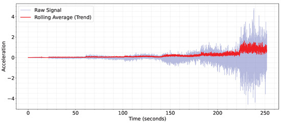 Figure 3. Visualization of speed steps in variable speed processes.
Each subset of the dataset was divided into training, validation, and test sets using an initial 60%-20%-20% split. Specifically, the constant speed phase included 28 processes for training, 10 for validation, and 10 for testing, while the variable speed phase comprised 36, 12, and 12 processes, respectively. This splitting procedure ensured that each subset was independent, with no process appearing in more than one subset. The original class distribution, in which the BPFO class contained twice as many samples as either the BSF or healthy classes, was preserved. To mitigate the effects of this class imbalance, a second, balanced version of the dataset was generated by downsampling the majority class to match the number of samples in the minority classes. This approach facilitates model training under conditions that minimize bias toward any particular fault type.
3.3. Feature Selection
The selection of features used as input for our models was performed gradually, with the goal of improving performance, and was guided by the specific challenges of fault detection and classification, as detailed in Section 4. The process leading to the final feature set can be divided into three main stages: (i) acceleration-only features, (ii) acceleration with envelope information, and (iii) statistical and spectral features in the time and frequency domains.
As described in Section 3.1, the testbench used for the creation of the dataset is equipped with two triaxial accelerometers. Consequently, the first set of features consisted of raw vibrational data along the x, y, and z axes for both bearings, capturing acceleration (m/s2) at each sampling instant, as can be seen in Figure 4. The raw data were segmented into windows of length 1000, resulting in an input tensor of shape , where the six channels correspond to the three axes from each sensor.
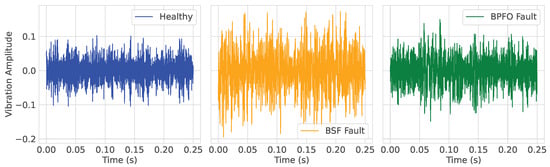
Figure 4.
Acceleration data for a sample of each class in the dataset.
While raw acceleration captures instantaneous vibrations, it is often insufficient to fully characterize fault-related phenomena, as different fault types may not be clearly distinguishable in the raw time-domain signal. To address this, the second feature set includes the signal envelope for each axis and each bearing, thereby providing information on amplitude modulations, as shown in Figure 5. The envelope of a signal is typically obtained by means of the analytic signal, defined as
where denotes the Hilbert transform. The envelope is then
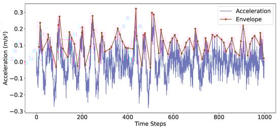
Figure 5.
Example of acceleration and envelope on one axis.
This smooth curve outlines the amplitude variations over time, effectively suppressing the high-frequency oscillations. Studying the envelope is crucial for condition monitoring because many mechanical anomalies (e.g., bearing defects, misalignments) manifest primarily as changes in amplitude rather than frequency [39,40]. The inclusion of these features doubled the dimensionality of the input, yielding a final tensor of shape .
To further improve model accuracy, we carried out an additional round of feature engineering aimed at identifying features with higher discriminative power. In this step, we explored non-linear transformations in both the time and frequency domains, while time-domain features capture overall signal behavior through statistical descriptors, the frequency domain is particularly important in ball bearing fault prediction because defects often generate characteristic vibration patterns at specific frequencies (e.g., fault frequencies linked to bearing geometry). These patterns are not always evident in the raw time signal but become more distinct once transformed into the frequency spectrum.
As a result, the final feature set combines time-domain statistical descriptors with frequency-domain characteristics, allowing us to better highlight differences between healthy and faulty conditions, as illustrated in Figure 6.
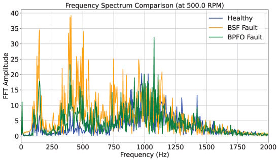
Figure 6.
Frequency between 0 and 2000 Hz for each class in the dataset.
For each axis, the following features were computed:
- Root Mean Square (RMS): quantifies the signal’s power, defined for a window asAn increase in RMS typically indicates higher energy in the vibration, often associated with faults.
- Crest Factor (CF): ratio of the maximum amplitude to the RMS, highlighting impulsive events:
- Kurtosis (): a normalized fourth central moment, capturing the “peakedness” of the distribution:where and are the mean and standard deviation, respectively. High kurtosis is a strong indicator of early-stage bearing faults.
- Skewness (): a measure of distribution asymmetry, given byDeviations from zero may signal asymmetric defect-induced vibrations.
- Spectral Peaks: the ten dominant frequency components were extracted from the magnitude spectrum of the Fast Fourier Transform (FFT). For each segment of length , the FFT is computed asand the largest ten magnitudes are retained as features, representing recurring periodicities linked to mechanical faults.
Combining these features results in 14 features per axis, leading to a total of 84 features per window across the six channels. A summary of all features used during the three steps is shown in Table 3.
Table 3.
Summary of extracted features for bearing fault diagnosis.
3.4. Models
The modeling approach was designed to evolve in parallel with the feature selection process. The models were built gradually, starting with simpler constant-speed measurements, where operating conditions are more stable. Once satisfactory performance and reliability were achieved, variable-speed measurements were introduced, allowing the models to adapt to non-stationary dynamics and enabling the refinement of both the architecture and its hyperparameters.
First, a CNN trained exclusively on acceleration-based features was developed to establish a baseline architecture. CNNs are feed-forward neural networks that employ convolutional filters to learn local patterns within structured data. By sharing weights across spatial or temporal dimensions, they efficiently detect translation-invariant features while maintaining a manageable number of parameters. This makes them particularly effective for vibration signals, where localized oscillatory patterns often correspond to specific fault conditions. Nonetheless, their limited capacity to model long-term temporal dependencies reduces their suitability for scenarios involving non-constant system behaviour, in which local feature extraction alone is insufficient.
The CNN was subsequently retrained with the inclusion of the envelope features, and later with a balanced version of the dataset obtained through undersampling to ensure all fault classes were equally represented. At each stage, the model was fine-tuned to maintain stable training behavior and achieve consistent benchmark performance. This progressive refinement led to a CNN architecture composed of three 1D convolutional blocks, each followed by max pooling and dropout layers to reduce dimensionality and mitigate overfitting. The convolutional filters, with a kernel size of 5, were designed to capture local variations in the vibration signal. The extracted feature maps were then flattened and passed through a fully connected layer before classification via a softmax output layer. The final structure of the CNN model is summarized as follows:
- Conv1D (128 filters, kernel size 5) + MaxPooling1D (pool size 3) + Dropout (0.5)
- Conv1D (64 filters, kernel size 5) + MaxPooling1D (pool size 3) + Dropout (0.5)
- Conv1D (32 filters, kernel size 5) + MaxPooling1D (pool size 3) + Dropout (0.5)
- Flatten + Dense(32, ReLU) + Dropout (0.5)
- Output: Dense (num_classes, Softmax)
With the addition of variable speed runs, the modeling framework was extended to include a hybrid architecture combining convolutional and recurrent layers. The CNN–BiLSTM model first employs convolutional and pooling layers to extract and compress local features, followed by a bidirectional Long Short-Term Memory (BiLSTM) layer that captures temporal relationships in both forward and backward directions. In doing so, it addresses the baseline CNN’s limitations by incorporating long-range temporal context that is necessary under non-constant operating conditions, combining it with spatially localized features extracted by convolutional layers. Dropout layers are used after both convolutional and recurrent stages to reduce overfitting. The structure of the CNN–BiLSTM model is summarized as follows:
- Conv1D (32 filters, kernel size 5) + MaxPooling1D (pool size 2)
- Conv1D (64 filters, kernel size 5) + MaxPooling1D (pool size 2) + Dropout (0.5)
- Bidirectional LSTM (64 units) + Dropout (0.5)
- Output: Dense (num_classes, Softmax)
These two architectures were selected to explore the benefits of combining convolutional and recurrent processing in a unified framework. Each model underwent a pre-training phase for hyperparameter tuning to identify the best-performing configuration.
Finally, to further enhance robustness and generalization, a Deep Ensemble learning strategy was applied to the best model identified in the previous step. Multiple instances of the model were trained with different random initializations, and their predictions were aggregated at inference time. Ensemble learning reduces variance, improves stability, and mitigates overfitting, while retaining the modeling advantages of the underlying architecture.
4. Results
This section presents the classification results obtained across all experimental settings. Alongside the proposed architectures, we also report results obtained using standard deep-learning baselines (LSTM, BiLSTM, ResNet, and Transformer) to provide a clear comparison and contextualize the gains achieved by the hybrid and convolutional approaches. To ensure a fair and unbiased comparison across all model families, we performed systematic hyperparameter tuning using Keras Tuner, applying the same search strategy and comparable search budgets (15 configurations, 30 epochs each) to both the baseline and proposed models. This procedure guarantees that each architecture is evaluated under well-optimized configurations, addressing concerns regarding model selection and hyperparameter fairness. For each experimental setting, we highlight the most relevant trends and discuss how different model families respond to variations in signal representation, class distribution, and operating speed.
4.1. Classification
4.1.1. Stage 1: Constant-Speed Evaluation
Table 4 summarizes the performance obtained when training exclusively on acceleration signals under constant-speed conditions. The results reveal a clear hierarchy among the tested architectures. Pure recurrent models (LSTM and BiLSTM) exhibit the lowest performance, reflecting their limited ability to extract meaningful fault-related patterns solely from raw vibration data. The CNN model, by contrast, achieves substantially higher accuracy (87.2%), highlighting the importance of convolutional filtering for capturing local temporal dependencies. The Transformer model also demonstrates competitive performance (96.6%), indicating that attention-based mechanisms can effectively model long-range interactions even in the absence of additional signal transformations. The CNN-BiLSTM architecture achieves near-perfect classification (99.4%), benefiting from the complementary strengths of convolutional feature extraction and bidirectional temporal modeling. ResNet attains the highest accuracy (99.9%), confirming the effectiveness of deep residual representations for fault classification under stationary operating conditions.
Table 4.
Accuracy comparison on Constant Speed using only acceleration. Best results are in bold.
The inclusion of envelope features (Table 5) leads to substantial improvements for most architectures. CNN performance increases to 97.0%, illustrating the relevance of demodulated vibration information for fault detection. Both CNN-BiLSTM and ResNet achieve nearly perfect scores, underscoring their ability to capitalize on the enriched representation. Interestingly, the Transformer exhibits a decrease in performance compared with the raw-acceleration setting, suggesting that its attention mechanisms may not benefit as directly from envelope information or may require additional feature tuning.
Table 5.
Accuracy comparison on Constant Speed using acceleration and envelope. Best results are in bold.
When the dataset is balanced to mitigate class imbalance (Table 6), its impact on the models is heterogeneous. CNN and ResNet maintain near-perfect accuracy, demonstrating strong generalization capability regardless of class distribution. In contrast, recurrent models (LSTM and BiLSTM) experience a significant degradation in performance, dropping to approximately 60% accuracy. This indicates a strong dependence on the original class priors and a limited ability to generalize when these priors are equalized, but also the need for more training data with respect to convolutional models. A plausible explanation for this drop is that recurrent models rely more strongly on temporal dependencies, which become less distinctive once class frequencies are equalized, rendering them more sensitive to changes in data distribution. CNN-BiLSTM also suffers a notable decrease, although it still outperforms the purely recurrent architectures.
Table 6.
Accuracy comparison on Constant Speed after balancing the dataset. Best results are in bold.
4.1.2. Stage 2: Variable-Speed Evaluation
The introduction of variable-speed data (0–5000 RPM) poses a more challenging classification scenario due to nonstationary effects. As shown in Table 7, all models exhibit reduced performance compared with the constant-speed case. Nonetheless, CNN-BiLSTM remains the best-performing architecture (93.7%), demonstrating resilience to temporal variability and speed-dependent spectral shifts. CNN also maintains strong results, whereas ResNet, despite its excellent performance under constant-speed conditions, shows a more pronounced drop, suggesting that its deep convolutional filters are less invariant to speed-induced distortions. Transformer and LSTM again yield the lowest accuracy values, reflecting limited adaptability to highly variable input dynamics.
Table 7.
Accuracy comparison on Variable Speed using acceleration and envelope. Best results are in bold.
4.1.3. Stage 3: Feature Engineering and Ensemble Learning
The adoption of advanced time- and frequency-domain descriptors (Table 8) significantly enhances performance across nearly all architectures. CNN attains 95.8% accuracy, confirming the benefit of engineered features instead of raw time-series representations. BiLSTM and especially CNN-BiLSTM show substantial gains, with the latter achieving 99.0%, indicating that hybrid architectures can effectively integrate both learned and handcrafted representations. ResNet also improves markedly, reaching 98.1%, which suggests that engineered spectral indicators mitigate the sensitivity of convolutional filters to speed-induced variability.
Table 8.
Accuracy comparison on Variable Speed using advanced feature extraction. Best results are in bold.
The Deep Ensemble approach, consisting of training five CNN-BiLSTM models and averaging their outputs, achieves the highest overall performance, reaching 99.3% accuracy, recall, and F1-score. This result highlights the advantages of model averaging in reducing variance, increasing robustness, and producing more stable predictions under real-world, variable-speed operating conditions.
Overall, the results clearly demonstrate that convolution-based architectures, especially the CNN-BiLSTM approach, when combined with engineered features or ensemble learning offer superior generalization and robustness across both constant-speed and variable-speed operating conditions.
4.2. Uncertainty Estimation
To enhance the interpretability and reliability of the model’s predictions, we implemented two complementary approaches to quantify uncertainty: MC Dropout and Deep Ensemble learning. Both methods allow the user to go beyond single-point predictions by providing not only an expected output but also a measure of confidence in the prediction.
MC Dropout involves enabling dropout during inference, a mechanism typically used only during training. By performing multiple stochastic forward passes for the same input, the network effectively produces a distribution of outputs. In our experiments, we generated 100 predictions per input sample. Each forward pass randomly deactivates a fraction of neural connections, creating slightly different models and thus capturing model uncertainty. From these 100 outputs, we compute the mean prediction and the standard deviation , representing the confidence of the network. Correct predictions generally show a low standard deviation (high confidence), while incorrect or ambiguous predictions exhibit higher dispersion. This allows end users to define thresholds on to trigger alarms or request human intervention, mitigating the risk of blind reliance on the model.
As illustrated in Figure 7, the uncertainty metric effectively differentiates between reliable and uncertain predictions. For a correct classification, the mean prediction is strongly concentrated on the correct class, and the standard deviation is nearly zero, signifying high confidence and robustness. Conversely, for a misclassified sample, the mean prediction is distributed across multiple classes (BSF has the highest mean probability, but is not the true class), and the large vertical error bars clearly indicate a high standard deviation . This correlation between high and misclassification confirms the value of using uncertainty to enhance the trustworthiness of the AI system, particularly when dealing with complex, non-stationary data.
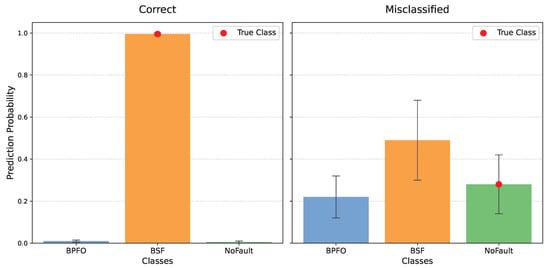
Figure 7.
Predictions made using MC Dropout approach on two test samples.
In addition to MC Dropout, we applied a Deep Ensemble strategy, combining predictions from multiple independently trained CNN-BiLSTM models. Each model produces its own output for a given input, and the ensemble prediction is obtained by averaging these outputs. Similar to MC Dropout, the standard deviation across the ensemble serves as an uncertainty measure, highlighting cases where the models disagree.
The ability of Deep Ensembles to provide reliable measures of predictive uncertainty is demonstrated by examining the probability distributions of predictions for correctly classified and misclassified samples. Figure 8 and Figure 9 present boxplots of the ensemble prediction probabilities under these two scenarios, allowing for a direct comparison of confidence levels and dispersion across classes.
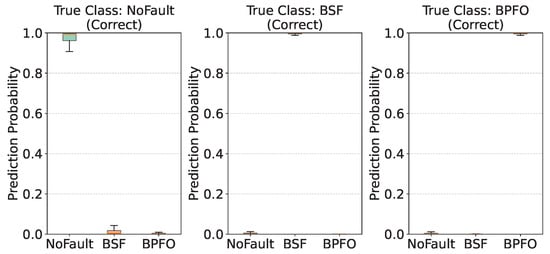
Figure 8.
Uncertainty distribution in correctly classified samples for each class using Deep Ensemble.

Figure 9.
Uncertainty distribution in misclassified samples for each class using Deep Ensemble.
Figure 8 illustrates the prediction distributions when the ensemble correctly identified the true class. In these cases, the predicted probability for the correct class is highly concentrated, with the median probability lying effectively at 1.0 across all three true classes. This indicates an ensemble prediction of high confidence. Moreover, the boxplots for the true class are extremely narrow, revealing minimal variance in the predictions among ensemble members. Such a low level of dispersion demonstrates consistent agreement across the ensemble and reflects an extremely low epistemic uncertainty. In practice, this consistency signifies that the ensemble classification is not only correct but also highly robust and trustworthy.
In contrast, Figure 9 depicts prediction distributions for samples that the ensemble misclassified. Unlike the sharp concentration observed for correct classifications, the distributions here display a much wider spread, with visibly larger interquartile ranges and greater overall variability. This increased dispersion corresponds to high predictive uncertainty, arising from disagreement among the ensemble members. Thus, high variance effectively serves as a built-in alert mechanism, signalling instances where the model is less reliable and where human review may be required.
Another key feature of the misclassified cases is the splitting of probability mass across multiple classes. For example, in the case of samples truly belonging to the BSF class but incorrectly classified, the ensemble’s probability mass was concentrated instead around the NoFault class, with a median predicted probability of approximately 0.63. Similarly, for true BPFO samples, the ensemble often assigned the highest probability to NoFault, with a median around 0.61. In both cases, the true class probability was not only lower but also subject to greater uncertainty (e.g., BSF samples had a median predicted probability for their true class of only 0.25). Such behaviour highlights how uncertainty manifests in practical error cases: the ensemble struggles to reach consensus, spreading its predictions across competing classes.
4.3. Explainable AI
To further increase the transparency of the model’s decision-making process, moving the system toward a “grey-box” approach, we utilized Shapley Additive Explanations (SHAP). Based on cooperative game theory, SHAP is a model-agnostic method that assigns an importance value (the SHAP value) to each feature, quantifying its contribution (positive or negative) to the final prediction for a given sample, relative to the average model output.
The SHAP analysis provides global insights into which features were most influential in achieving the final ensemble accuracy of 99.3% (Table 8). The results are presented in two summary plots, grouping features by bearing and by feature type.
Figure 10 provides a high-level comparison of the feature importance aggregated by the sensor location: ACC1 All Features (Bearing 1) versus ACC2 All Features (Bearing 2). In a SHAP summary plot, features are ranked by the average magnitude of their impact, and the color represents the feature’s actual value (red for high, blue for low).
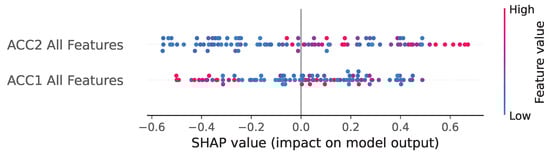
Figure 10.
SHAP analysis at bearing level.
The plot indicates that, across the entire dataset, features from ACC2 All Features have a consistently greater overall impact on the model’s prediction than those from ACC1. This suggests that the vibrational characteristics measured at the second bearing position were slightly more discriminative for fault diagnosis; indeed, it is where the faulty bearing was placed in our measurements.
A more granular breakdown is presented in Figure 11, which groups the features into their specific domain categories: Time Features (RMS, Crest Factor, kurtosis, skewness) and Frequency Features (spectral peaks).
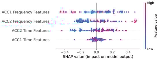
Figure 11.
SHAP analysis at feature level.
This analysis strongly validates the feature engineering strategy detailed in Section 3.3 and the performance results in Section 4.1:
- Dominance of Frequency Features: the ACC1 Frequency Features and ACC2 Frequency Features groups exhibit the largest SHAP value magnitudes. This confirms that the spectral components, which directly correspond to the physical fault frequencies (BPFO and BSF), are the primary drivers of the model’s high diagnostic accuracy. The model correctly prioritizes these domain-expert-derived features to distinguish between different fault types.
- Role of Time-Domain Features: while significant, the ACC1 Time Features and ACC2 Time Features groups show a comparatively lower overall impact. This indicates that traditional time-domain statistical descriptors, such as kurtosis, play a necessary but secondary role. They likely contribute to detecting the existence of an impulsive event (early-stage fault detection) and general severity (via RMS), but the frequency features are essential for accurate classification of the fault type.
By correlating the high SHAP values associated with the frequency-domain features with the spectral density analysis shown in Figure 12 and Figure 13, restricting the comparison to processes operating at 500 RPM to ensure coherence, we observe that the model’s decision boundary is primarily influenced by signal magnitude within the structural resonance bands. Figure 12 reveals a multimodal distribution shared by all three classes in the 500 Hz and 800–1000 Hz regions, reflecting the inherent structural resonances of the machinery. In contrast, the faulty classes exhibit an additional spectral component in the 300–400 Hz band that is absent in the healthy state.
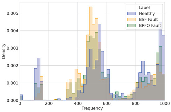
Figure 12.
Analysis of dominant frequencies in processes operating at 500 RPM.
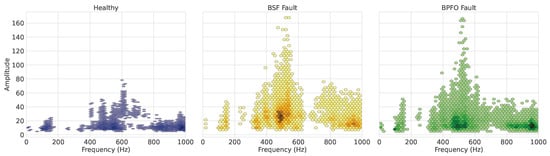
Figure 13.
Analysis of signal amplitude in processes operating at 500 RPM.
Although the frequency locations of the dominant peaks substantially overlap across classes, Figure 13 indicates that signal amplitude serves as the key discriminative factor. The healthy class is characterized by low-magnitude vibrations across all resonance bands, whereas both fault conditions display a pronounced increase in spectral energy. In particular, the BSF class shows the highest concentration of spectral density in the 500 Hz band, suggesting that this fault induces a narrowband excitation that strongly couples with the machine’s natural frequency. Conversely, the BPFO class exhibits a broader distribution of high-energy peaks within the 400–600 Hz range, consistent with the more impulsive, wide-band excitation typically associated with outer-race defects.
4.4. Model Training and Inference Performance
Table 9 summarizes the computational characteristics of the evaluated models on the extended dataset using the complete feature set, reporting their training time, inference time, and number of trainable parameters. Overall, ResNet and the CNN variants, show the lowest computational cost, fast inference and relatively small parameter counts. Recurrent models exhibit higher training and inference times, particularly the bidirectional variants, which roughly double the computational load compared to their unidirectional counterparts. The Transformer model presents the highest training time among the deep architectures, reflecting its increased complexity despite a moderate parameter count.
Table 9.
Summary of model computational metrics.
5. Conclusions
In this study, we introduced a new rolling bearing vibration dataset that captures healthy and faulty conditions under both constant and variable speeds, including ball pass frequency outer race and ball spin frequency defects. Using this dataset, we developed a CNN-based fault classification framework enhanced with white-box feature selection, incorporating raw acceleration, envelope, and time- and frequency-domain statistical descriptors.
Experimental results demonstrate that raw acceleration signals alone provide sufficient information to distinguish healthy from faulty bearings (87.2% accuracy) under constant speed, but additional features are essential for accurately classifying fault types. Incorporating envelopes improves performance conditions (97.0%), while balancing the dataset further increases accuracy to 99.9%.
Under variable-speed conditions, classification complexity increases, highlighting the need for robust architectures; a CNN-BiLSTM hybrid with advanced features achieves 98.7%, and a Deep Ensemble strategy reaches 99.3% accuracy.
Moreover, MC Dropout and Deep Ensemble effectively quantifies prediction uncertainty, offering confidence measures that can guide maintenance decisions. SHAP analysis was used to confirm the dominance of frequency-domain features in fault discrimination, validating the grey-box approach. Overall, the proposed methodology provides a robust, interpretable, and high-performing framework for industrial predictive maintenance.
Future research will pursue several complementary directions aimed at enhancing the performance and generalization capabilities of the proposed model. A primary focus will be the development of an improved version of the dataset, incorporating more heterogeneous data, including additional defect types as well as the same defects exhibited at varying levels of severity. This expanded dataset is expected to enable the model to capture subtle variations in defect patterns and improve robustness across a wider spectrum of operational conditions. Subsequently, the model will be evaluated under real-world conditions, providing critical insights into the model’s ability to generalize beyond the controlled laboratory environment used during training.
On the methodological front, future work will explore alternative deep learning architectures, including attention-based models beyond the transformer architectures already tested. Additionally, domain adaptation techniques, such as Domain-Adversarial Neural Networks (DANNs), will be investigated to facilitate knowledge transfer across datasets with differing characteristics, improving performance especially on smaller datasets, tackling the problem of costly data acquisition campaigns.
Author Contributions
Conceptualization, L.M., P.E., and L.C.; Methodology L.M., P.E., and A.M.; Supervision L.C. All authors have read and agreed to the published version of the manuscript.
Funding
This study was carried out within the MICS (Made in Italy—Circular and Sustainable) Extended Partnership and received funding from Next-Generation EU (Italian PNRR—M4 C2, Invest 1.3—D.D. 1551.11-10-2022, PE00000004). CUP MICS D43C22003120001.
Data Availability Statement
The raw data supporting the conclusions of this article will be made available by the authors on request.
Conflicts of Interest
The authors declare no conflicts of interest.
References
- Cristaldi, L.; Esmaili, P.; Gruosso, G.; La Bella, A.; Mecella, M.; Scattolini, R.; Arman, A.; Susto, G.A.; Tanca, L. The mics project: A data science pipeline for industry 4.0 applications. In Proceedings of the 2023 IEEE International Conference on Metrology for eXtended Reality, Artificial Intelligence and Neural Engineering (MetroXRAINE), Milano, Italy, 25–27 October 2023; IEEE: New York, NY, USA, 2023; pp. 427–431. [Google Scholar]
- Vashishtha, G.; Chauhan, S.; Sehri, M.; Zimroz, R.; Dumond, P.; Kumar, R.; Gupta, M.K. A roadmap to fault diagnosis of industrial machines via machine learning: A brief review. Measurement 2025, 242, 116216. [Google Scholar] [CrossRef]
- Rehman, A.U.; Jiao, W.; Jiang, Y.; Wei, J.; Sohaib, M.; Sun, J.; Rehman, K.U.; Chi, Y. Deep learning in industrial machinery: A critical review of bearing fault classification methods. Appl. Soft Comput. 2025, 171, 112785. [Google Scholar] [CrossRef]
- Afshar, M.; Heydarzadeh, M.; Akin, B. A comprehensive investigation of fault signatures and spectrum analysis of vibration signals in distributed bearing faults. IEEE Trans. Ind. Appl. 2024, 61, 515–526. [Google Scholar] [CrossRef]
- Martiri, L.; Esmaili, P.; Cristaldi, L. A Novel Benchmark for Fault Detection in Rolling Bearings Using CNNs and Monte Carlo Dropout. In Proceedings of the 2025 IEEE International Workshop on Metrology for Industry 4.0 & IoT (MetroInd4.0 & IoT), Castelldefels, Spain, 1–3 July 2025; pp. 462–466. [Google Scholar]
- Esmaili, P.; Cristaldi, L. Health indicator analysis in terms of condition monitoring on brownfield cnc milling machines using triaxial accelerometer. IEEE Sens. Lett. 2024, 8, 6008404. [Google Scholar] [CrossRef]
- Randall, R.B.; Antoni, J. Rolling element bearing diagnostics—A tutorial. Mech. Syst. Signal Process. 2011, 25, 485–520. [Google Scholar] [CrossRef]
- Althubaiti, A.; Elasha, F.; Teixeira, J.A. Fault diagnosis and health management of bearings in rotating equipment based on vibration analysis—A review. J. Vibroeng. 2022, 24, 46–74. [Google Scholar] [CrossRef]
- Esmaili, P.; Cristaldi, L. Health indicator effectiveness in localized fault diagnosis: Rolling bearing elements. In Proceedings of the 2024 IEEE International Workshop on Metrology for Industry 4.0 & IoT (MetroInd 4.0 & IoT), Firenze, Italy, 29–31 May 2024; pp. 552–556. [Google Scholar]
- Antoni, J. Cyclostationarity by examples. IEEE Trans. Instrum. Meas. 2016, 65, 1256–1264. [Google Scholar] [CrossRef]
- He, W.; Shen, Q.; Sun, S. Envelope analysis-based diagnosis of bearing defects under variable speed conditions. IEEE Trans. Ind. Electron. 2016, 63, 5682–5692. [Google Scholar]
- Song, S.; Wang, W. Early Fault Detection of Rolling Bearings Based on Time-Varying Filtering Empirical Mode Decomposition and Adaptive Multipoint Optimal Minimum Entropy Deconvolution Adjusted. Entropy 2023, 25, 1452. [Google Scholar] [CrossRef]
- Sandoval Núñez, D.A.; Leturiondo, U.; Vidal, Y.; Pozo, F. Entropy Indicators: An Approach for Low-Speed Bearing Diagnosis. Sensors 2021, 21, 849. [Google Scholar] [CrossRef]
- Yang, X.; Yang, J.; Jin, Y.; Liu, Z. A New Method for Bearing Fault Diagnosis across Machines Based on Envelope Spectrum and Conditional Metric Learning. Sensors 2024, 24, 2674. [Google Scholar] [CrossRef] [PubMed]
- Ruiz-Sarrio, J.E.; Antonino-Daviu, A.; Martís, C. Localized Bearing Fault Analysis for Different Induction Machine Start-Up Modes via Vibration Time–Frequency Envelope Spectrum. Sensors 2024, 24, 6935. [Google Scholar] [CrossRef] [PubMed]
- Tang, S.; Yuan, S.; Zhu, Y. Cyclostationary Analysis towards Fault Diagnosis of Rotating Machinery: Review, Advances, and Challenges. Processes 2020, 8, 1217. [Google Scholar] [CrossRef]
- Martiri, L.; Esmaili, P.; Cristaldi, L. A Convolutional Neural Network for CNC Milling Machines Processes Classification. In Proceedings of the 2024 IEEE International Conference on Metrology for eXtended Reality, Artificial Intelligence and Neural Engineering (MetroXRAINE), St Albans, UK, 21–23 October 2024; IEEE: New York, NY, USA, 2024; pp. 634–639. [Google Scholar]
- Wan, L.; Gong, K.; Zhang, G.; Yuan, X.; Li, C.; Deng, X. An efficient rolling bearing fault diagnosis method based on spark and improved random forest algorithm. IEEE Access 2021, 9, 37866–37882. [Google Scholar] [CrossRef]
- Hang, Q.; Yang, J.; Xing, L. Diagnosis of rolling bearing based on classification for high dimensional unbalanced data. IEEE Access 2019, 7, 79159–79172. [Google Scholar] [CrossRef]
- Janjarasjitt, S. Investigating the Effect of Vibration Signal Length on Bearing Fault Classification Using Wavelet Scattering Transform. Sensors 2025, 25, 699. [Google Scholar] [CrossRef]
- Jabbar, A.; D’Elia, G.; Cocconcelli, M. Distribution Reshaping Transformation for Bearing Fault Diagnosis in Independent Cart Systems. IEEE Access 2025, 13, 200403–200430. [Google Scholar] [CrossRef]
- Wang, H.; Yu, Z.; Guo, L. Real-time online fault diagnosis of rolling bearings based on KNN algorithm. In Proceedings of the 2019 4th International Seminar on Computer Technology, Mechanical and Electrical Engineering (ISCME 2019), Chengdu, China, 13–15 December 2019; Journal of Physics: Conference Series. IOP Publishing: Bristol, UK, 2020; Volume 1486, p. 032019. [Google Scholar]
- Lu, Q.; Shen, X.; Wang, X.; Li, M.; Li, J.; Zhang, M. Fault diagnosis of rolling bearing based on improved VMD and KNN. Math. Probl. Eng. 2021, 2021, 2530315. [Google Scholar] [CrossRef]
- Zhao, B.; Zhang, X.; Li, H.; Yang, Z. Intelligent fault diagnosis of rolling bearings based on normalized CNN considering data imbalance and variable working conditions. Knowl.-Based Syst. 2020, 199, 105971. [Google Scholar] [CrossRef]
- Zheng, X.; Liu, X.; Zhu, C.; Wang, J.; Zhang, J. Fault diagnosis of variable speed bearing based on EMDOS-DCCNN model. J. Vib. Eng. Technol. 2024, 12, 7193–7207. [Google Scholar] [CrossRef]
- Guo, Y.; Mao, J.; Zhao, M. Rolling bearing fault diagnosis method based on attention CNN and BiLSTM network. Neural Process. Lett. 2023, 55, 3377–3410. [Google Scholar] [CrossRef]
- Öcalan, G.; Türkoğlu, İ. Diagnosis of Bearing Faults Under Variable Speed Conditions Using Deep Learning. Veri Bilim. 2025, 8, 1–10. [Google Scholar]
- Liu, H.; Zhou, J.; Zheng, Y.; Jiang, W.; Zhang, Y. Fault diagnosis of rolling bearings with recurrent neural network-based autoencoders. Isa Trans. 2018, 77, 167–178. [Google Scholar] [CrossRef] [PubMed]
- Bearing Data Center. Bearing Data Center Website. 2019. Available online: https://engineering.case.edu/bearingdatacenter (accessed on 13 November 2025).
- Nectoux, P.; Gouriveau, R.; Medjaher, K.; Ramasso, E.; Chebel-Morello, B.; Zerhouni, N.; Varnier, C. PRONOSTIA: An experimental platform for bearings accelerated degradation tests. In Proceedings of the IEEE International Conference on Prognostics and Health Management, PHM’12, Denver, CO, USA, 18–21 June 2012; pp. 1–8. [Google Scholar]
- Jabbar, A.; Cocconcelli, M.; D’Elia, G.; Borghi, D.; Capelli, L.; Cavalaglio Camargo Molano, J.; Strozzi, M.; Rubini, R. MOIRA-UNIMORE Bearing Data Set for Independent Cart Systems. Appl. Sci. 2025, 15, 3691. [Google Scholar] [CrossRef]
- Daga, A.P.; Fasana, A.; Marchesiello, S.; Garibaldi, L. The Politecnico di Torino rolling bearing test rig: Description and analysis of open access data. Mech. Syst. Signal Process. 2019, 120, 252–273. [Google Scholar] [CrossRef]
- Lee, J.; Qiu, H.; Yu, G.; Lin, J.; Services, R.T. Bearing Data Set. IMS, University of Cincinnati. NASA Prognostics Data Repository, NASA Ames Research Center, Moffett Field, CA. 2007. Available online: https://phm-datasets.s3.amazonaws.com/NASA/4.+Bearings.zip (accessed on 13 November 2025).
- Huang, H.; Baddour, N. Bearing vibration data collected under time-varying rotational speed conditions. Data Brief 2018, 21, 1745–1749. [Google Scholar] [CrossRef]
- Gal, Y.; Ghahramani, Z. Dropout as a bayesian approximation: Representing model uncertainty in deep learning. In Proceedings of the International Conference on Machine Learning. PMLR, New York, NY, USA, 19–24 June 2016; pp. 1050–1059. [Google Scholar]
- Abdar, M.; Pourpanah, F.; Hussain, S.; Rezazadegan, D.; Liu, L.; Ghavamzadeh, M.; Fieguth, P.; Cao, X.; Khosravi, A.; Acharya, U.R.; et al. A review of uncertainty quantification in deep learning: Techniques, applications and challenges. Inf. Fusion 2021, 76, 243–297. [Google Scholar] [CrossRef]
- Ganaie, M.A.; Hu, M.; Malik, A.K.; Tanveer, M.; Suganthan, P.N. Ensemble deep learning: A review. Eng. Appl. Artif. Intell. 2022, 115, 105151. [Google Scholar] [CrossRef]
- Mohammed, A.; Kora, R. A comprehensive review on ensemble deep learning: Opportunities and challenges. J. King Saud Univ. Comput. Inf. Sci. 2023, 35, 757–774. [Google Scholar] [CrossRef]
- Areias, I.A.d.S.; Borges da Silva, L.E.; Bonaldi, E.L.; de Lacerda de Oliveira, L.E.; Lambert-Torres, G.; Bernardes, V.A. Evaluation of current signature in bearing defects by envelope analysis of the vibration in induction motors. Energies 2019, 12, 4029. [Google Scholar] [CrossRef]
- Randall, R.B.; Antoni, J.; Chobsaard, S. The relationship between spectral correlation and envelope analysis in the diagnostics of bearing faults and other cyclostationary machine signals. Mech. Syst. Signal Process. 2001, 15, 945–962. [Google Scholar] [CrossRef]
Disclaimer/Publisher’s Note: The statements, opinions and data contained in all publications are solely those of the individual author(s) and contributor(s) and not of MDPI and/or the editor(s). MDPI and/or the editor(s) disclaim responsibility for any injury to people or property resulting from any ideas, methods, instructions or products referred to in the content. |
© 2025 by the authors. Licensee MDPI, Basel, Switzerland. This article is an open access article distributed under the terms and conditions of the Creative Commons Attribution (CC BY) license (https://creativecommons.org/licenses/by/4.0/).