Fast Infrared Detector for Time-Domain Astronomy

Abstract

Multi-messenger astronomy and time-domain astronomy are strongly linked even if they do not have the same objectives. Multi-messenger astronomy is an astrophysical observation approach born by the simultaneous, even if casual, detection of a few events discovered up to now. In contrast, time-domain astronomy is a recent technological trend that aims to make observations to explore the sky not with imaging, astrometry, photometry or spectroscopy but through the fast dynamic behavior of celestial objects. Time-domain astronomy aims to detect events on a temporal scale between seconds and nanoseconds. In this paper, a time-domain infrared fast detector for ground-based telescopes is proposed. This instrument can be useful for multi-messenger observations, and it is able to detect fast astronomical signals in the order of 1 ns. It is based on HgCdTe photoconductors, but the InAsSb photovoltaic detector has also been tested. The detection system designed to detect fast mid-infrared bursts includes trigger modules, an off-line noise-canceling strategy, and a classifier of the transients. Classification is derived from the analysis of fast instabilities in particle circular accelerators. This paper aims to be a preliminary feasibility study.

1. Introduction

Electromagnetic transients (i.e., electromagnetic signals that emerge rapidly over a relatively short time, less than a few seconds) from cosmic sources provide a wealth of information about astrophysical objects. Their observations in different electromagnetic ranges constitute an important part of modern astrophysical research such as, for example, the case of fast radio bursts [1,2]. Moreover, Hauser and Dwek [3] analyzed the cosmic infrared background discovering radio–infrared background connection. In fact, data from the IRAS (InfraRed Astronomical Satellite) revealed a remarkable correlation between radio and infrared (IR) fluxes from galaxies, stretching over four orders of magnitude in IR flux density [4].

Following these studies, an instrument based on a time-resolved mid-infrared (mid-IR) detector, developed for diagnostics in accelerator physics, is proposed for applications in time-domain and multi-messenger astronomy to acquire fast mid-IR bursts. In the next sections, the proposal of a temporal device for astronomy is presented as a design study about an ultra-fast IR time-resolved detector suitable for ground-based telescopes. The objective of this article is to shortly present a scientific scenario, preliminary design concepts and tests to be evaluated for a following feasibility study report.

Implementation of the detection system in the focal plane of a reflecting telescope will be used to search for possible astronomical fast infrared bursts (FIRBs). FIRBs are astronomical events that have been relatively understudied, often due to the lack of appropriate tools for observation and analysis. Being based on a telescope, the instrument will also be capable of identifying the direction of the source of bursts, particularly useful in multi-messenger astronomy.

Section 1.1, “A new astronomy”, presents a short introduction to multi-messenger and time-domain astronomy. This is to insert the proposal in a scientific scenario to justify R&D for the instrument under study.

The instrument’s basic design concepts for approaching the objective are presented in Section 2. DAFNE (Double Annular Φ-Factory for Nice Experiments), a lepton circular accelerator and e+/e- collider of the Istituto Nazionale di Fisica Nucleare (INFN) hosted at the Laboratori Nazionali di Frascati (LNF), is briefly introduced. Some aspects of diagnostics for charged particle accelerators are presented together with an introduction on how to characterize fast instabilities of the e+/e- beams acquired using the diagnostic devices. The infrared beamline SINBAD, emitting pulsed synchrotron radiation, has been used for testing the front-end of the detection system.

Time-resolved infrared detection is analyzed in Section 3. The project is based on the evaluations of HgCdTe and InAsSb semiconductor technologies. The implementation is discussed including design activities, circuits developed, ground-based telescope options and design blocks.

Test and performance results are described in Section 4. The results of the tests carried out at the LNF are reported with an analysis of detector performance.

Further design aspects for the final implementation are presented in the same chapter about other important telescope features:

• An analysis of different algorithms proposed for generating automatic triggers to enable data acquisition;
• Programs developed for emulating astronomical bursts with the goal of generating a preliminary database of possible transients;
• Software tools developed for burst classification by using pattern recognition (PR) techniques developed for artificial intelligence (AI);
• Considerations about the possible noise-canceling strategy;
• Considerations about the future use of artificial neural networks for pattern recognition.

A general discussion of the critical aspects of the experiment is reported in Section 5.

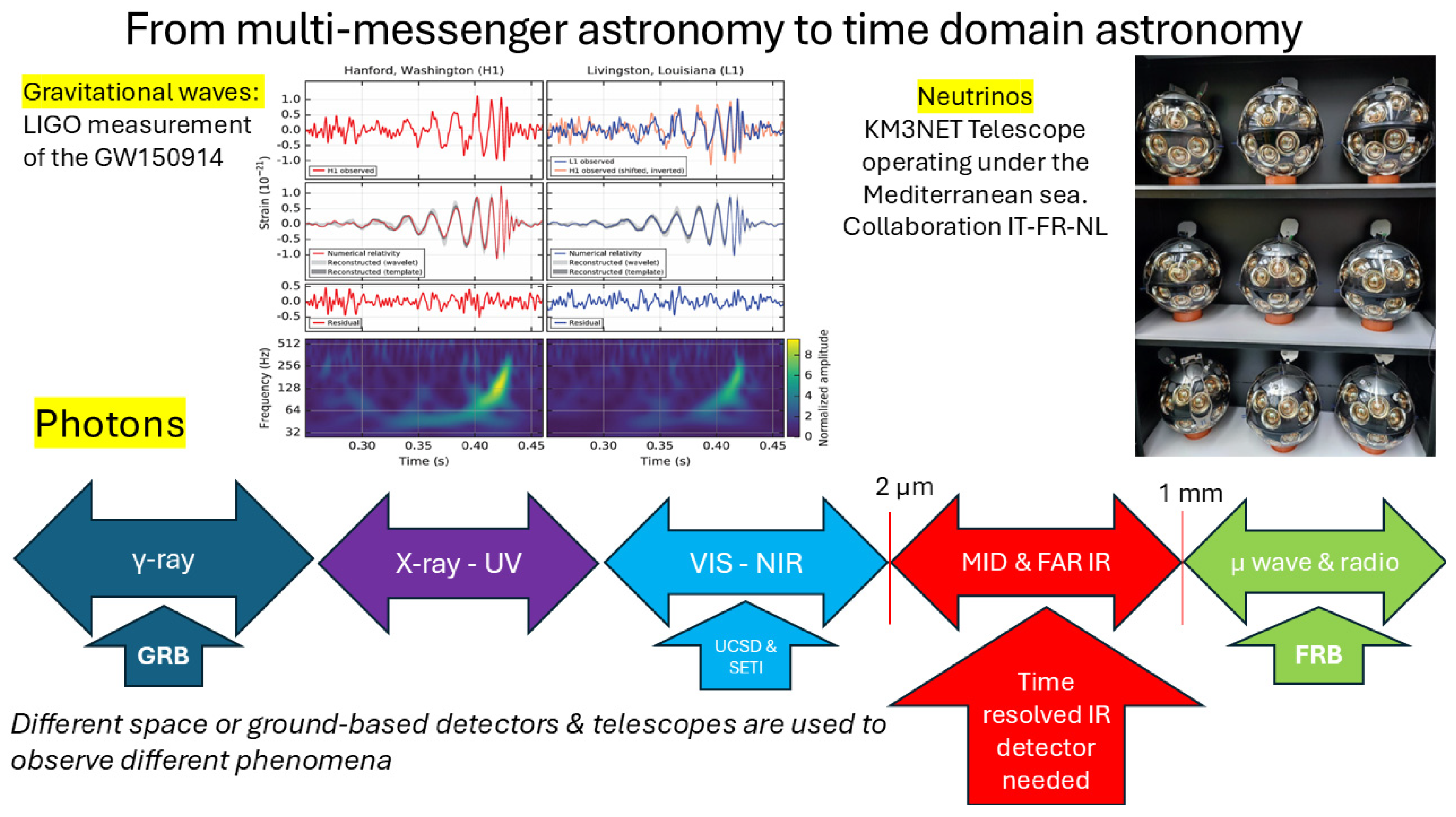
1.1. A New Astronomy

After Galileo, the evolution of astronomical knowledge has been profoundly related to the instruments used. The increasing acceleration of the number of discoveries that has occurred in recent decades requires new approaches to design detection systems. Gravitational wave telescopes, gamma-ray burst monitors and fast radio burst telescopes have raised great interest in multi-messenger and time-domain astronomy. In the following discussion, some considerations are presented with the aim of justifying the proposal of an innovative ground-based telescope dedicated to temporal and directional observations of fast astronomical events in the middle infrared spectrum.

1.1.1. Fast Radio Bursts

Fast Radio Bursts (FRBs) are very interesting astronomical transients. An astronomical transient is broadly defined as any event that appears and fades on a time scale observable by humans [5] or smaller. A FRB is a radio frequency transient lasting between a fraction of a millisecond and 3 s. Many FRBs oscillate around 1400 MHz; some have been detected at lower frequencies in the range of 400–800 MHz [6]. Given their implied small emitting regions and large distances [7,8], FRBs should be generated by perfect point sources and still appear point-like when they arrive in the Milky Way [9].

Up to 2019, FRBs had only been detected in the radio band; no contemporaneous infrared signal had been observed, while few cases of simultaneous optical, X-ray or gamma-ray flash had been detected [10,11,12].

In 2019, there were at least 55 published progenitor theories for FRBs. No dominant theory has emerged about the sources of FRBs in the recent literature, where many different interpretations of these phenomena have been proposed. Possible sources of fast bursts, radio or infrared [13] are collected and discussed in the web catalog https://frbtheorycat.org and in the Transient Name Server https://www.wis-tns.org/ (both sites accessed on 7 May 2025).

Among the many hypotheses, it is worth mentioning the transition from black hole to white hole hypothesized by Hal Haggard and Carlo Rovelli in 2015, based on considerations of the quantum nature of General Relativity in the article “Black Hole Fireworks: Quantum-gravity Effects Outside the Horizon Spark Black to White Tunnelling” [14]. Another article, “Fast Radio Bursts and White Hole Signals” by Barrau, Rovelli, and Vidotto [15], states the following:

“A strong explosion in a small region should emit a signal with a wavelength of the order of the size of the region or somehow larger and convert some fraction of its energy in photons. Therefore, it is reasonable to expect an electromagnetic signal emitted in the infrared from this scenario:

λ predicted ≥ 0.02 cm.”

A wavelength of 200 µm is not that far from the operative range of the detector proposed in this research. Carlo Rovelli, in a private communication [16], did not exclude cases with shorter λ in the mid-infrared, but he stated that calculations should be made.

As a conclusion to this section, the possible models proposed for the explanation of FRBs can in many cases be revised or adapted for astronomical photons of different energy, for example, in the infrared range. This could be the case of the model proposed for white holes [17,18].

1.1.2. Time-Domain Astronomy

Considering that time-domain astronomy spans over time scales from a few seconds to 1 ns (2–3 s to 10⁻⁹ s), dedicated detectors for telescopes need to be designed [19]. Furthermore, different types of systems are necessary to observe gravitational waves (GWs), neutrinos and photons in different ranges of the electromagnetic spectrum (see Figure 1). In fact, the present research is focused on the mid-infrared (mid-IR) part of the electromagnetic spectrum: more exactly, from 2 to 12 μm wavelength.

Lastly, in the time-domain astronomy research, the Einstein Probe (EP), launched on 9 January 2024 and entering the operational phase starting around mid-June of 2024, must not be forgotten. The EP, not to be confused with the NASA’s Einstein Observatory, is an X-ray space telescope mission by the Chinese Academy of Sciences (CAS) in partnership with the European Space Agency (ESA) and the Max Planck Institute for Extraterrestrial Physics (MPE) dedicated to time-domain high-energy astrophysics [20]. The primary goals are “to discover high-energy transients and monitor variable objects”. EP mission objectives are “searching the Universe for cosmic variable objects and transient phenomena shining in X-ray light”.

Figure 1. Time-domain astronomy involves gravitational waves, neutrinos and electromagnetic radiations in all energy ranges. Top left image credit: Abbott et al. 2016, [21]. Top right image credit: https://web.infn.it/ (accessed on 7 May 2025).

Figure 1. Time-domain astronomy involves gravitational waves, neutrinos and electromagnetic radiations in all energy ranges. Top left image credit: Abbott et al. 2016, [21]. Top right image credit: https://web.infn.it/ (accessed on 7 May 2025).

1.1.3. Directionality of the Detection

The Einstein Telescope, a proposed third-generation GW observatory [22], is explicitly designed with features to better identify the astronomical coordinates of the GW source. The importance of this feature is such that it deeply influences the very design of the observatory, based on two interferometers with L-shaped arms or a triangular scheme with three arms. Considering the interest in identifying the direction of bursts, it is useful to design a direction pointing device.

To summarize, multi-messenger astronomy pushes technology toward new detectors with directional capability and temporal response in the order of µs or ns. In the infrared range, the technologies implemented up to now do not really seem suitable to approach this type of objective. A completely different type of approach and detection system is necessary to search for ultra-fast infrared bursts (see Figure 2).

2. Instrument Design Basic Concepts

2.1. The Interstellar Medium as a Particle Accelerator

Enrico Fermi was the first scientist to describe the Interstellar Medium (ISM) as an accelerator of charged particles. He proposed mechanisms that are now called Fermi’s First and Second accelerator laws, hence the idea of applying the technology of diagnostic devices developed for particle accelerators to astronomical observations for detecting fast bursts and transients.

In order to design a new type of astronomical detector in the mid-infrared range, the experience gathered in the lepton beam diagnostics for circular particle accelerators can be useful. In the jargon of accelerator physics, diagnostic devices integrating over time to take images of beams are called transverse, while those acquiring in the time domain are called longitudinal [23,24]. For longitudinal devices, the time delay of a charged particle bunch is referred to as the accelerator master clock. In a first approximation, one bunch, containing typically 10⁷–10¹⁰ particles, is considered rigid in its center of mass. Hence, longitudinal diagnostic devices need to acquire only the time position of the barycenter of each single bunch versus the expected bucket position. A bucket is an electromagnetic potential well, moving close to the light speed. A bucket may contain a bunch of particles or may be empty.

2.2. DAFNE and SINBAD

At the LNF of the INFN, DAFNE, an electron/positron circular accelerator and collider operating since 1998 [25], is available for pulsed synchrotron light experiments. The accelerator is composed of a linac (linear accelerator), a damping ring, transfer lines, two main rings, two interaction regions and several UV, X and IR beamlines. The two main rings have a length of 97.6 m, with 510 Mev energy, 368.667 MHz radio frequency (f_RF) and 120 buckets. In the interaction regions, positron and electron bunches collide at an energy of 1.02 GeV in the mass center. Although the energy of DAFNE is fixed, beamlines are available for experiments with photons of different energies.

A time-domain (or longitudinal) detection system to be implemented for astronomical observations using ground-based telescopes or scientific balloons has been tested at SINBAD [26], the infrared light beamline [27] of DAFNE. At SINBAD, the electron beam, stored in a ring, emits bunches of infrared photons generated by synchrotron acceleration from a dipole-bending electromagnet connected to a pipe of a few meters through an exit port. The electron beam is split into bunches by the radiofrequency system that restores energy losses, and, as consequence, emitted synchrotron light is also pulsed in a 2.7 ns period (=1/f_RF). In reality, the charge is distributed only in a small part of the bucket, and, consequently, the rise time and fall time of the infrared signal are ≤ 1 ns. This is a very useful feature for testing fast, time-resolved detectors.

2.3. Diagnostics for Circular Accelerators

To be operative, a circular particle accelerator needs many diagnostic devices. Some devices work in transverse and others work in longitudinal or time-domain mode with different goals. The electron beam image, acquired by integrating visible light using a synchrotron light monitor, does not show any presence of bunches. On the contrary, a high-frequency oscilloscope displays particle bunch signals from electromagnetic pickups connected to the instrument inputs as shown in Figure 3. The oscilloscope shows the amplitude of the two beams, positrons (in red) and electrons (in blue), versus time. Figure 3 highlights the separation in bunches made by the radio frequency system. The 2.7 ns distance between the buckets corresponds to the radio frequency period.

2.4. Particle Beam Fast Instabilities

The stored particle beam can suffer from many types of instabilities. In this article addressed to astrophysics, the interest in beam instabilities is due to the fact that their behavior is similar to astronomical transients. From the point of view of diagnostics for the accelerators, it is important to acquire fast instability behavior with the goal of characterizing and classifying it, as well as to measure, if possible, the growth rate [28]. In a storage ring, it is necessary to control and/or mitigate the instabilities of the beam, which is split into bunches of charged particles [29].

A time-domain or longitudinal diagnostic device for particle accelerators is usually designed by sampling the analog signals coming from electromagnetic or optical pickups at a frequency inversely correlated to the bunch distance. Each bunch usually has a Gaussian shape in the three dimensions, horizontal, vertical and longitudinal planes, even with different sizes. Note that, to correctly maintain synchronization with the phase of the bunches, the source of the sampling frequency must be the same as that of the machine master clock. This is to avoid undesired and inevitable instrumental phase shifts.

The information acquired by sampling the analog signal in correspondence to the barycenter of each bunch will be the quantity of charge and the oscillation amplitude with respect to the equilibrium point in the three dimensions, longitudinal, horizontal and vertical. This implies that three detection systems are necessary; but, with the perspective of the present astrophysical telescope design project, only the longitudinal or temporal oscillations are considered. A phase detector is used to acquire longitudinal signals. The phase difference is measured with respect to the accelerator master clock. For each dimension, the instability growth rate will be calculated by acquiring the difference from the rest position of each bunch in a convenient number of turns. This is similar to considering n harmonic oscillators described by n ordinary differential equations (ODEs) of a second order, as expressed in Formula (1):

d²τ_n/dt² + 2 ∗ d_r ∗ dτ_n/dt + ω_s² ∗ τ_n = F

(1)

where

• τ = the difference in time with respect to the rest position;
• n = the bunch number;
• d_r = the radiation damping factor = 1/(growth rate);
• ω_s = the angular frequency of the synchrotron oscillations;
• F = the force generating the instability effect.

In a storage ring, it is also possible to measure the “modal” growth rate given that in a circular accelerator the number of modes is correlated with the number of buckets (called the harmonic number). Formula (2) can be used to calculate the number of buckets in a storage ring, considering that the leptons are relativistic and travel nearly at the light speed:

N_b = R_L ∗ f_RF/c

(2)

where

• N_b = number of buckets;
• R_L = ring length;
• f_RF = radio frequency;
• c = speed of light.

For DAFNE, the following applies:

N_b = (97.6 m ∗ 368.667 MHz)/(299 792 458 m/s) = 120 buckets

However, the concept of modal growth rate does not seem so easily applicable to the astrophysical transient case. In fact, the number of modes is probably unknown or extremely large. A theoretical model will be necessary, but after the acquisition of real transients.

Since, from an astrophysical point of view, the interest is measuring the growth rate of instability, calculation of the growth coefficient versus time of the beam considered as a whole, omitting any modes, is sufficient to characterize this behavior. In reality, approximation using the harmonic oscillator model could also be inadequate for astrophysical signals. In the software to emulate transients (see Section 4.4.1), several cases are considered: square/exponential, single pulse and pulse train, Gaussian and triangular shapes, noise in the absence of a real signal and no signal.

2.5. Trigger to Record the Instabilities

Given that the data memory cannot be infinite, it is also necessary to define a starting signal for the data acquisition, called the “trigger”.

In diagnostics for a particle accelerator, the trigger can be the following:

• Generated by the machine master clock;
• Generated by bunch injection into the ring;
• Correlated with arising instability.

Case 3 requires a smart approach for trigger generation. It must be underlined that, in a particle storage ring, a beam instability can be excited in various ways. For example, the simplest way is turning off the bunch-by-bunch feedback that controls the coupled bunch oscillations [28]. Alternatively, it is possible to vary the current of an electromagnet or excite the beam with white noise or sinusoidal signals.

In addition, in a circular collider, an instability can also occur or be damped by shifting the orbits of the two beams at the collision point [30]. Synchrotron oscillations produce time arrival differences with respect to the master clock.

All of these possible ways to excite instability can be correlated with using a dedicated pulse generator equipped with an auxiliary trigger output.

Considering the case of detecting fast astronomical signals, the problem is much more complex because a master clock does not exist and the sampling frequency should vary based on the type of event. However, there is a maximum reasonable value for the sampling frequency based on the detection system bandwidth and capability. Considering the Nyquist–Shannon sampling theorem and searching for signals with 1 ns rise time, the sampling frequency must be at least 4 Gsamples/s.

For astronomical events, the choice of trigger is more complicated to avoid wasting data memory or operator time. The design of the trigger for the telescope will be discussed in Section 4.3.

2.6. How to Identify the Instability Source

There is no simple recipe for identifying the source of an instability in a circular accelerator; however, measuring the growth rate and identifying the excited mode can help pinpoint the source. The puzzle can be solved because a circular accelerator is a human creation made by a finite number of pieces. The number of oscillating modes, if the bunch is rigid, will be equal to the number of buckets, so it is a finite number. Practically, mechanical and thermal inspections can be carried out to understand if there is any broken or critical part. The growth rate is an important clue. Theoretical or numerical electromagnetic models of each piece of the storage ring are used to evaluate their contribution to instability. This is performed by means of a quantity called “machine impedance” [31,32].

Comparing fast instabilities in circular accelerators to fast transients observed in astronomy can be thought of as an analogy. Both phenomena can be acquired, recorded and analyzed to identify possible types and localization of the source by knowing the rise time, shape and amplitude of the observed transient signal.

3. Time-Resolved Infrared Detection

3.1. Basics of the Project

Designing an infrared telescope to search for fast astronomical transients requires a different approach from standard infrared telescopes. First, the signal cannot be integrated; it has to be acquired in real time and in single shot. This excludes bolometers or similar integrating devices, as well as multi-pixel detectors that are intrinsically slower because they have to manage a large flux of data to be stored in memory. Considering signals with a rise time of the order of 1 ns brings the design choice in the direction of a detector based on a single pixel with time-resolved capability. In addition, another identical detector, dedicated to acquiring environmental and instrumental noise (the “dark” signal or D signal), is implemented in the design to avoid recording insignificant signals. The dark signal detection system must be identical to the detection system used for the astronomical signal (A signal), avoiding a different detectivity in the device bandwidth, both within and outside the mid-infrared range considered (2–12 µm). In fact, commercial product data sheets often indicate the detector specifications in the frequency bandwidth that is declared operative, but they do not explain what happens outside the operative range. The second detector implemented for acquiring the D signal is convenient for evaluating noise that affects the astronomical signal both in and outside the operative bandwidth in real time.

3.2. Synchrotron Radiation Infrared Beamline

The SINBAD beamline is available to test detectors for fast infrared signals with a 1 ns rise time. It is a good choice, even if it has limitations due to some difference in the expected astronomical signals.

The need to have infrared light pulsed with a 1 ns rise time and fall time is satisfied because each bunch of charged particles emits pulsed infrared radiation through synchrotron acceleration. The particle bunch has a Gaussian shape and, to be stable, must be shorter than the 1.35 ns half-period of the bucket. However, even if the timing structure of the photons emitted through synchrotron acceleration corresponds to the timing structure of the particle bunches, the photons emitted by SINBAD are spread in a large energy range, while the electrons have a much smaller energy spread. Also, the IR light intensity versus wavelength varies during the unavoidable beam current variations [27].

The JWST MIRI, like many other telescopes, has available bandpass filters with wide and narrow bandwidths that are selected during data taking. On the contrary, during data collection with SINBAD, it was not possible to apply any filter in the infrared range. This fact entails some limitations in the tests carried out. In fact, the SINBAD beamline emits infrared photons with a wide energy spread, including sub-mm photons, too. As a consequence, it is very difficult to be sure that the detector does not acquire noise or spurious signals outside the 2–12 µs bandwidth considered. In Section 4.5, a discussion on noise-canceling strategy is reported. In addition, other tests, performed by putting the photoconductor inside the DAFNE hall where the particle beams are circulating, have demonstrated that strong radiofrequency fields can produce coherent and incoherent noise that produces undesired effects outside the declared operative frequency bandwidth of photodetectors.

3.3. HgCdTe Detectors

In recent years, the research on HgCdTe (or MCT, mercury cadmium telluride) semiconductors for infrared photodetectors made great technological progress [33,34,35]. However, fast, time-resolved detection systems have not been considered really useful for astronomy, because experiments were mainly oriented to integrate signals rather than for time-domain detection.

HgCdTe is a chemical compound of cadmium telluride (CdTe) and mercury telluride (HgTe) with a tunable bandgap energy, spanning the short waves to the very long waves in the infrared region. CdTe is a semiconductor with a bandgap of approximately 1.5 eV at room temperature. HgTe is semimetal, and its bandgap energy is zero. Mixing these two substances allows one to obtain any bandgap between 0 and 1.5 eV. Solid solutions of Hg_1–xCd_xTe are widely used for the development of infrared photoelectronic devices. The amount of cadmium in the alloy can be chosen to match the optical absorption of the material to the desired infrared wavelength, and the x factor reports the percentage of CdTe vs. HgTe in the solid solution. In photodetectors based on MCT, both materials of a small composition, with x ≈ 0.2–0.3, and wider-band compositions, with x ≈ 0.5–0.7, are currently used, as in the present experiment.

For the objective of the proposed telescope, major advances have been made in MCT detectors with time-resolving capability and devices operating at room temperature, with improvements in characteristics [36]. Other tested technological solutions are based on InAsSb and they are discussed in Section 3.4.

MCT time-resolved photodetectors can reproduce a fast rise time and fall time of infrared signals. MCT photodetectors can be photoconductive or photovoltaic, but photovoltaic devices have a slower response for technological reasons. The room temperature-operating feature is a relatively new and very important characteristic. Previous infrared devices needed to be cooled to maintain a low level of thermal noise in the semiconductor. In the following sections, tests are reported to validate the room temperature performance by making a comparison between cases, with or without the Peltier’s cells.

Studies about the application of time-resolved MCT mid-IR photodetectors in diagnostics for accelerator physics have been carried out at the infrared beamline of the DAFNE electron ring [37,38].

To summarize, photodetectors based on semiconductor technologies can be proposed for fast astronomical transients. The required main features are as follows:

• Fast response to the inputs, in the order of 1 ns.
• Good specific detectivity D* and responsivity R in the mid-IR range selected for the telescope (2–12 µm) where D* is defined as

  D* = ((A ∗ Δf)^1/2/NEP),

  where A is the active detector area, Δf is the frequency interval and NEP is the Noise-Equivalent Power.
  The photodetector responsivity R is given in Ampere per incident radiant power (A/W) units and is

  R = (η ∗ q)/(h ∗ f)

  where η is the quantum efficiency, q is the electron charge, h is the Plank constant and f is the frequency of the optical signal.
• Low noise.
• Operating at room temperature (preferably): this feature makes a ground-based telescope more compact and easily transportable, even if the use of Peltier’s cells would be a practical solution.

Furthermore, the detection system should be as compact as possible for use as a mobile or transportable device and for easy placement in the focal plane of the telescope.

The HgCdTe detectors tested are photoconductors made by VIGO Photonics S.A. [39] that have been chosen because they accomplish the required specifications in terms of detectivity and frequency response at room temperature (see Figure 4). In addition, photoconductors have a faster rise time than photovoltaic devices.

The VIGO PC series consists of 1.0–12.0 µm HgCdTe ambient-temperature photoconductive detectors that feature uncooled IR photoconductive detectors. The devices are optimized for maximum performance at λ_opt. Performance at low frequencies is reduced due to 1/f noise. The 1/f noise corner frequency increases with the cut-off wavelength.

The Vigo Catalog includes photovoltaic, photoelectromagnetic and photoconductor devices. However, considering the need for time-resolved detection with a 1 ns rise/fall time, the photoconductors are the best choice. The spectral response detectivity D* versus wavelength of the PC10.6 photoconductor is shown in Figure 4.

It is worth noting that even if the PC10.6 device has been declared to have a detectivity peak at 10.6 µm, the real peak seems to be between 7 and 9 µm. However, the shape of the response curve is spread from 1 to 12 µm.

3.4. InAsSb Detectors

Another semiconductor technology, based on InAsSb, has been evaluated. The working range is usually considered more suitable for wavelengths shorter than 5 µm, in near-infrared (NIR), but recent progresses by many producers has extended the working range to mid-IR. Indeed, as shown by the Hamamatsu data sheet of the P13894 series products [40], the detection seems to be as good as that of HgCdTe technology. The spectral operating range is between 2.5 µm and 11 µm. InAsSb photodetectors have the advantages of being less expensive and made by substances that are environmentally compatible with the RoHS Directive. From the point of view of ambient temperature, it must be noted that the detector’s performance works better at −30 °C than at 25 °C or 60 °C.

4. Tests and Results

In July 2021, the author of the present paper proposed, as the principal investigator, the FAIRTEL (Fast InfraRed TELescope) experiment to the National Scientific Commission 5 (CSN5) of the Italian National Institute of Nuclear Physics (INFN). Based on previous experiments carried out on IR diagnostics for accelerator physics, the FAIRTEL experiment aims to build a detection system designed for ground-based astronomy observations. The detection system aims to be able to detect fast and ultra-fast mid-infrared astronomical transients or bursts. The experiment wishes to place the detector in the focal plane of a reflecting telescope, such as Ritchey–Chrétien or Cassegrain. The choice of a reflecting telescope is mainly due to the fact that it makes the focusing operation easier. The implementation of scientific balloons has been considered as well.

4.1. Front End Analog Module

Using photoconductors, a transimpedance circuit is necessary to adapt the electrical signal from current to voltage. This conversion is necessary for using voltage amplifiers working at a radio frequency. A high frequency bias-tee has been used to implement the transimpedance circuit to interface with the voltage amplifier. Circuits for a single-pixel and multi-pixel front end have been designed and tested at the LNF at the SINBAD beamline [41,42,43].

For the multi-pixel detection, the PCB, with dimensions of a cellular phone (7 × 14 cm), can host up to 19 pixels with the TO-39 case, a transistor package.

The PCB designed at the LNF can allow the placement of up to 19 pixels, all used in time-domain mode, not for imaging. They are put in two parallel connections on the board to increase the two output signals (A and D). Alternatively, 19 single outputs can also be generated using a flat connector with 20 pins × 3 lines. Each pixel corresponds to a PC-10.6 photoconductor, with the TO-39 package, while the BNC0type package is incompatible with the PCB even if it is electrically identical. The analog front end, including a transimpedance circuit, is completed by an external amplification stage. RF amplifiers with bandwidths up to 4 GHz are implemented. The analog front end is the most critical part of the telescope for transients. Astronomical data are recorded by a fast data acquisition system that needs a trigger module and off-line post-processing software, described in the following sections.

4.1.1. Test Carried Out at SINBAD

At the infrared SINBAD beamline, front end circuits have been tested to accomplish the specification required by the project. Figure 5 shows an oscilloscope plot, where the MCT detector signal (cyan trace; 2 mV per division) is amplified by 20 dB, reproducing the infrared light pulse train corresponding to the electron bunch train signal from an electromagnetic pickup (yellow trace of the oscilloscope). The red trace shows the machine master clock used as a trigger. The difference in phase is not meaningful, because it is due to different lengths in the signal paths.

4.1.2. Performance of HgCdTe Detectors

To evaluate performance versus temperature, tests were carried out to compare the behavior of the VIGO detectors both at room temperature (RT) and at lower temperatures. This was performed using two Peltier cells as a sandwich, with the device in the middle. No difference was found in the noise level, showing that cooling is not necessary for this series of HgCdTe detectors.

In summary, using pulsed synchrotron light from SINBAD, several detectors and amplifiers were evaluated. HgCdTe photoconductors, even with different active areas or packages, showed excellent time-resolved performance, with fast light IR pulses of a 1 ns rise time. The only drawback was that the transimpedance circuit ruled out the use of the detector in the low frequency band of the transient, below ~10 kHz.

The evaluation of detector detectivity was carried out using infrared synchrotron light of the SINBAD beamline. The photon source comes from a bending magnet with a magnetic field of 1.2 T. The energy of the emitted photons has a large spread, well outside the detector’s detectivity, specified by a maker from 2 to 12 μm in wavelength. The photon beam divergence is 17 mrad (horizontal) × 35 mrad (vertical). The declared photon FLUX is 10¹³ photons/s × 0.1% bandwidth, as reported by the beamline specifications [26]. The SINBAD photon flux is calculated as a total beam current of 2 A, which is usually the maximum stored current of the electron beam. However, time-resolved detectors, unlike bolometers and similar integrating devices, are sensitive to the IR pulses emitted by each electron bunch in each turn, not to the total beam current. Some calculations are required.

The DAFNE harmonic number is 120, but to avoid the ion trapping effect, some buckets are left empty, storing usually in the ring a train of 100 bunches (Nb) followed by a gap of 20 empty slots. Hence, each bunch emits 10¹³/100 = 10¹¹ photons per second.

The 10¹¹ ph/s value must be divided by the revolution frequency f_REV; that is

f_REV = ~368 MHz/120 = 3.067 MHz

because the signal acquisition is made for one bunch in one turn. The result is that 32 k photons are emitted per each bunch, with a current of 20 mA in each turn and 3.2 k photons with a bunch current of 2 mA.

The measurements are taken during the electron/positron collisions, with a bunch current between 2 and 20 mA. In this range of bunch current, the detector signal is correctly displayed and measured (peak–peak voltage) using the oscilloscope. The performance, in terms of sensibility to the pulse, was found to be between 3.2 k and 32 k photons × 0.1% bw (δλ/λ) without saturation or distortion.

For a bunch of 2 mA, a peak-to-peak signal of 2 mV was measured after 20 dB voltage amplification, which corresponds to a 0.2 mVpp detector output without any amplification.

Considering the realistic possibility for the engineered system to use an 80 dB amplification stage equivalent to a 10 k linear gain, the detection system shall be sensitive to 1 photon for 0.1% of the infrared bandwidth (δλ/λ) by using the needed 80 dB amplification.

Furthermore, as reported in [19], the rise and fall time for three bunches of the electron beam were measured using the uncooled IR photoconductor detector PC10.6-R005. The rise time and fall time of the IR signals were about 0.7 and 1 ns, respectively. The bunch current was ~14 mA. The signal was acquired from the pulsed IR synchrotron light, converted into electricity by the HgCdTe detector and amplified. To make this measurement, the signal was amplified using a 40 dB voltage amplifier with 10 kHz–4 GHz bandwidth.

4.1.3. Performance of InAsSb Detector

For comparison, a photovoltaic detector, based on a different and cheaper technology, an InAsSb semiconductor, was tested. Being photovoltaic, it does not require the transimpedance circuit and, for this reason, it can work at extremely low frequency. As a drawback, the photovoltaic technology shows smaller detectivity, about one third of the photoconductor, and more noise (10–20% more). The smaller signal response required the use of two 35 dB amplifiers for a total voltage gain of 70 dB to reach an amplitude at the level obtained using the MCT detector with a 20 dB amplification.

To try to decrease the thermal noise, the detector was put between two Peltier cells without obtaining appreciable improvement of the signal-to-noise ratio. This was carried out by using two Peltier cells as a sandwich with the device in the middle. No difference was found in the noise level, showing that cooling is not necessary for RT (room temperature) detectors.

The rise time and fall time of the photovoltaic detector, shown in Figure 6 (cyan trace), are less performant than the ones of MCT detectors. Testing the InAsSb photovoltaic detector at the synchrotron beamline and implementing the amplification stage using MiniCircuit ZFL1000-LN produces the result, in terms of time-domain response, shown in Figure 6. The photovoltaic device cannot compete with the HgCdTe photoconductor: only the envelope of the bunch train is visible, and separation between the bunches cannot be acquired. Furthermore, the signal is much noisier, as is evident in Figure 6, and the signal output amplitude, even after an amplification stage of 70 dB, is small.

However, the InAsSb photodetector can be useful in searching for slower astronomical transients, in the order of seconds or milliseconds, because this photovoltaic technology does not need the bias-tee circuit that acts as a high-pass filter.

4.2. Data Acquisition System

A state-of-the-art, though commercial, data acquisition system was planned for the final configuration. The analog-to-digital converters (ADCs) for digital acquisition have to be at least two, but preferably four: two ADCs for the A (astronomical) and D (dark) signals, one for the trigger, and one for a test input. ADCs with 12/14/16 bits are necessary to have an adequate dynamic range > 72dB, ruling out 8/10 bits converters.

The ADC sampling clock frequency should preferably be changeable by the operator. To acquire signals with a 1 ns rise time, a 4 GHz analog bandwidth and 10 Gsamples/s are desirable to best overcome and manage the Shannon–Nyquist sampling theorem in the acquisition system.

The module can be implemented by programming a dedicated data acquisition system. A very good solution, which satisfies specifications, is the ADQ7DC digitizer by Teledyne [44] with the following requested features: 10 samples/s; 14-bit vertical resolution; and two channels at 5 GSPS or one channel at 10 GSPS.

4.3. Trigger

Other modules have been developed to complete the design of the FAIRTEL telescope for the final implementation. Software programs have been written for the trigger module simulator, the burst emulator and the burst classifier.

At the present stage of the project, all the programs used for the trigger simulator, the FIRB emulator and the FIRB classifier are implemented by GNU Octave [45]. Used for scientific computing and numerical computation, it is mostly compatible with MATLAB, developed by MathWorks, Inc. [46]. As part of the GNU Project, GNU Octave is free software under the terms of the GNU General Public License.

In a subsequent future engineering phase, the trigger algorithms that need to react immediately to any incoming event should be written in C/C++ as procedural language or using VHDL/Verilog in case of implementation with a FPGA (Field-Programmable Gate Array).

4.3.1. Trigger Module Design

Triggers are necessary to record only astronomical transients presenting potential interest. They have to be analyzed offline, avoiding flooding real-time processing unit(s) and data memory. In fact, the acquisition system should always be running, but data recording should start only when one of the trigger modules enables it.

To better explain this point, it is useful to do some calculations. Supposing, for example, a FIRB of one second. The analog to digital conversion can be performed at 12 or 14 or 16 bits, which are all recorded as two bytes for the sample. Hence, storing 10 Gsamples/s for two channels in the memory requires 0.04 terabytes of memory space per second.

Without a reasonable trigger to enable data recording, in 24 h, the stored data would amount to 3456 terabytes, and in one year, it would amount to more than one million terabytes. The conclusion is that a trigger module is mandatory to start data logging.

To summarize, different types of triggers for starting data acquisition have to be implemented. First, for testing the devices at SINBAD or in the laboratory, the trigger will be one of the following:

• The machine master clock from the accelerator timing system during data collection at the infrared beamline.
• The sync output from a pulse generator in the case of signal simulation.

For astronomical observations, the situation is more complicated and requires alternative approaches that briefly can foresee the following:

• A trigger threshold level selected by the operator.
• A smart automatic trigger generated by the astronomical signal or by a comparison between the astronomical signal and the dark signal. It can be implemented in different ways that are discussed below. Basically, the software module must be designed to calculate a movable threshold level that, when exceeded, enables the trigger for data acquisition.
• A trigger forced by a command from the operator.
• An external trigger coming from other astronomical systems operating for multi-messenger astronomy.
• A self-diagnostics trigger via a pulse generator for testing purposes.

The threshold level must be extrapolated based on the environmental noise and thermal noise levels acquired by the dark signal detector, while making a comparison with the astronomical signal. The trigger threshold value, computed from the dark signal, must be averaged and updated in a short temporal range. A variable gain that can be applied to the background fit by the operator for increasing system flexibility is foreseen.

The Fermi-GBM detector provides a powerful example of triggers with 28 algorithms currently installed. In fact, Fermi-GBM Triggering Operations can be used as an example for developing trigger modules. However, note that FERMI-GBM has multiple detectors, while the FAIRTEL telescope has only one astronomical detector. The trigger starts when two or more detectors exceed a preset and adjustable threshold specified in units of the standard deviation of the background rate. The background rate is the average rate accumulated over the previous 17 s, excluding the most recent 4 s. Furthermore, the acquisition system can manage several timescales, from 16 ms to 8.192, with 28 algorithms installed [47].

In the FAIRTEL project, triggers for data acquisition activate the start of data recording; however, the size of the record file has to be determined, too. The number of samples in each record can be chosen through selection in one of three ways:

• Fixed data length based on the operator choice;
• Data record length limit based on technological considerations about the available data memory;
• Threshold comparison of the input value based on a percentage of trigger threshold (considering if the transient is terminated).

4.3.2. Trigger Modules

Given that the FAIRTEL telescope does not have multiple detectors like Fermi-GBM, it is necessary to compute the difference between the background fit for the A (astronomical) signal and the D (dark) signal in real time. To analyze the behavior of the smart trigger module, a software trigger simulator (trigger.m) has been written in OCTAVE language. Four smart triggers are simulated. Note that in all cases, the operator is asked for the number of loops for more simplicity. This is just to make the simulation reasonable, while, in the real procedure, the program runs forever.

The TRG1 smart trigger procedure will do the following:

• Select the trigger threshold value manually by operator.
• If the A signal is >threshold, start recording the acquisition.

The TRG2 smart trigger procedure will do the following:

• For every time slot, compute the D signal background average.
• Apply a gain factor to the D signal average to obtain the trigger threshold. The gain should be evaluated by the operator, but it is 1 by default. The gain factor should take care of the possible hardware discrepancy of the semiconductors or external noise.
• If the A signal is >threshold, start recording the acquisition.

The TRG3 smart trigger procedure will do the following:

• For every second, compute the A and D background average or fit in the last second.
• Calculate the average of the last five fits for both the A and D inputs.
• Evaluate the difference between the A- and D-averaged background.
• Apply a gain factor [0:2] to the difference result to obtain the trigger threshold. The gain should be evaluated by the operator, but it is 1 by default. The gain factor has to take care of the possible hardware discrepancy of the semiconductor.
• If the A signal is >threshold, start recording the acquisition.

The TRG4 smart trigger procedure will be as follows:

• For every time slot, compute the D background average.
• Add a delta value to the D average to obtain the trigger threshold.
• If the A signal is >threshold, start the recording of the acquisition.

4.4. Pattern Recognition Software for Transient Classification

The data acquisition system is completed by implementing dedicated software based on “standard” artificial intelligence (AI) techniques, more specifically pattern recognition (PR) techniques, an important branch of AI [48,49,50,51]. This approach is necessary because astronomical IR transients would most likely be extremely rare, with an unknown shape and rise time. The trigger module will select events that will be recorded together with observation data: time label and telescope pointing direction in equatorial coordinates in Epoch J2000.0. This ensures a stable database that can be analyzed for years. The transients will be stored to be evaluated offline by the classifier using both visual inspection and an automatic pattern recognition procedure. This approach keeps in mind the fast instability classification and analysis techniques used for lepton circular accelerators. In order to design a realistic classifier, it is necessary to preliminarily create a database including samples with different features.

4.4.1. Fast IR Burst Emulation

Testing of the FIRB classifier requires a database that is generated with an emulator, given that there are still no astronomical data. The emulator, written in a procedural language, is able to create a database of one-dimensional tracks (quantized amplitude versus discrete time) containing some of the possible foreseen transients with different degrees of noise and jitter and different values of amplitude, growth rates and shapes. A large database can easily be generated with the emulator.

The first provisional list of transient models is the following: single square pulse, pulse trains (variable or fixed amplitude and frequency, length, etc.) and other shapes like Gaussian, triangular, exponential, etc. The effect of a burst with an exponential growth rate is equalized to that of a square pulse because, from the detector’s point of view, the effect is to produce a very similar rise in the signal. Just as explained in Section 2.6, “How to identify the instability source” in a storage ring, knowing the characteristics of the burst does not allow us to easily identify the astronomical source but can provide clues about it.

To create a realistic database to be used to test the classifier, a transient emulator program FIRB_emulator.m, (Fast InfraRed Burst emulator) has been developed using Octave.

The identification of the possible astronomical sources generating fast infrared bursts will be investigated offline. Hence, the amplitude, shape, rise time and pulse repetition of prototypes for the transients have been generated with and without noise using algorithms in the emulator. This approach aims to create a database of various valid models used for training and testing the classifier. Each pattern is stored in a text-formatted file with each file name reporting the creation time. This allows us to easily manage each file in the database. Graphic pattern plots in .tiff format have been stored, too.

Filenames have the format year-month-day-hour-minute-second.txt, for example, “2024-7-31-18-0-36.txt”, reporting the file creation time. Other useful information about the event will be stored in a parallel text file with the same name but with a different extension (.info). The .info file includes pointing values in equatorial coordinates for Epoch J2000.0. This enables standardization of the data format. Other useful information to be stored in the .info file includes sampling frequency, operator name (if any), weather conditions, possible multi-messenger data links, comments and other information.

Several examples of patterns inserted in the database are shown in Figure 7. A first pattern, recorded as 2024-7-31-17-44-48.txt, reports a single square pulse with random noise. The amplitude is in mV versus the sample number. The sampling interval will be included in the .info file. In this way, all the plots do not define the temporal scale to maintain the best data flexibility in case of varying sampling frequency.

Random noise in each pattern can be added at the creation time with different amplitudes by changing the noise gain. The RAND function returns a vector with random elements uniformly distributed on the (0, 1) interval, which, after multiplication by the chosen noise gain, is added to the pattern created.

A second pattern (stored as 2024-7-31-13-13-20.txt) presents a train with ten squared pulses with noise. The number of pulses can be modified in the program as well as the number of samples.

In addition to square pulses, records of other types of acquired data are also present in the database and recognized by the classifier. Files 2024-7-31-18-24-20.txt and 2024-7-31-13-15-46.txt are Gaussian patterns without and with noise.

File 2024-7-31-18-0-36.txt (and .tiff) contains just uniform noise. The record has been inserted in the database because it presents a situation that can often be found by chance or mistake.

In Figure 7, in the top right corner, pattern 2024-7-31-18-15-49.txt and .tiff has a triangular shape. Even if a triangle can seem, at first look, too simple of a mathematical pattern, it can be a useful prototype to describe transients with slow and regular rise times that could be found.

4.4.2. Fast IR Burst Classification

After generating the pattern database, the burst classifier program was written and tested. The classifier is implemented using procedural approach software (Octave) but, differently from the previous emulator program, it can also be implemented using artificial neural networks (ANNs) with machine learning (ML) capability. The ML approach, still not implemented, is discussed in the following Section 4.6.

The FIRB_classifier.m program consists of three main steps:

• Ask the operator for the file name and read the selected record from the database, evaluating any possible format error. If the data format is correct, go to the next point.
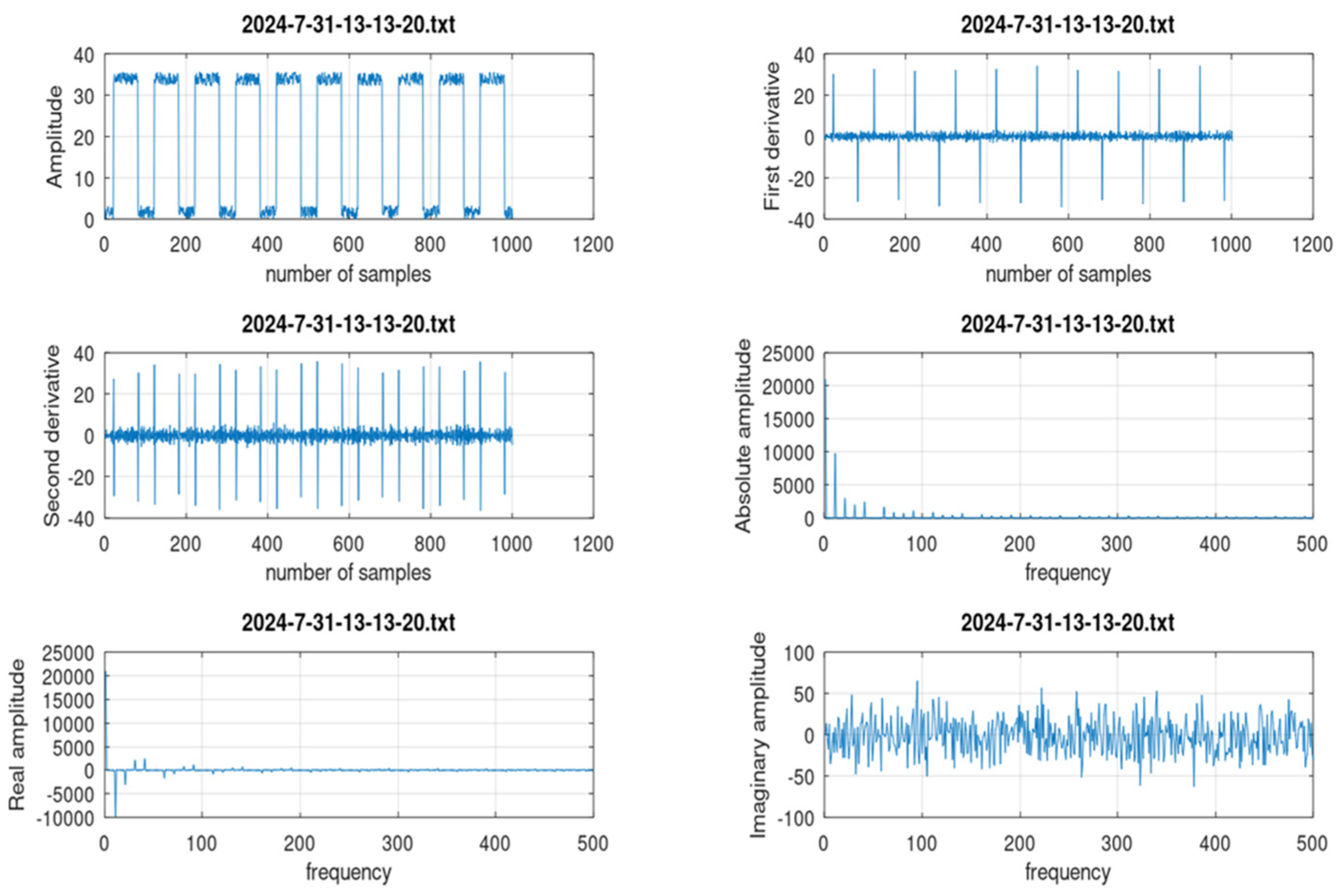
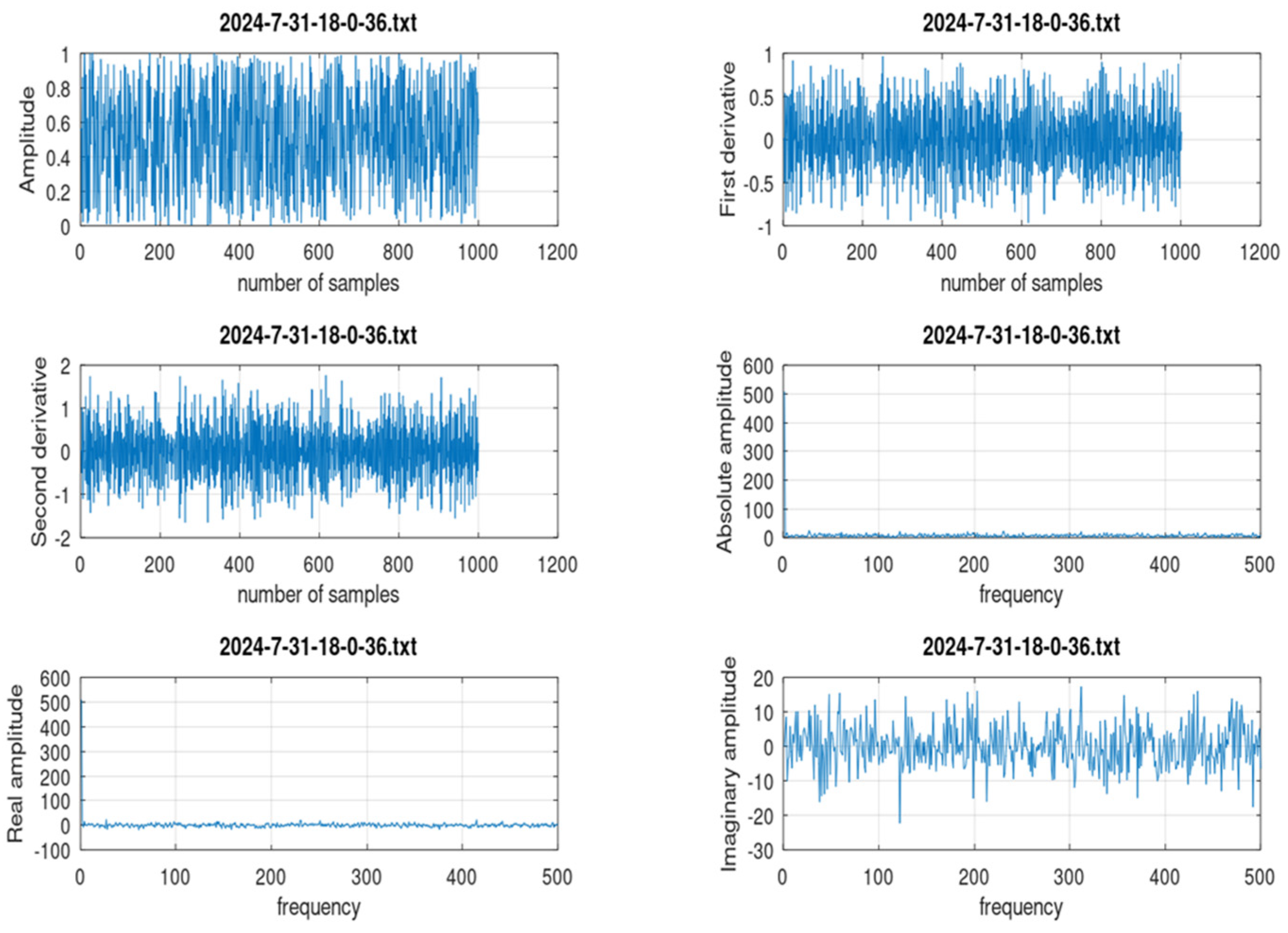
• Make a general analysis of the data of each transient, presenting a visual inspection in the time domain and the frequency domain.
• Classify the transient based on the amplitude and the growth rate.

The procedural approach manages “symbols” using “syntactic” rules to classify the signals based on their shapes [52]. This method is based on theorical considerations developed by pattern recognition (PR) techniques.

Briefly, every pattern has a meaning in a specific context. Astronomical transients, after recording, become patterns in a database. Patterns under investigation can be grouped into separated clusters in order to classify them. One or more clusters correspond to a class in which the peculiar features are determined and identified. A class should correspond to a specific astrophysical phenomenon, as a final goal.

PR techniques can be implemented with symbolic and procedural language or alternatively using ANNs after a preliminary ML stage.

The main difference in these two approaches is the training phase. By using the procedural language, the main “supposed” features are embedded in the program through the implementation of pattern characteristics by the programmer before writing the PR classification program. On the contrary, the ANN/ML approach needs a large database to start the machine learning training phase. For these reasons, the development of a PR procedural program is more suitable in a preliminary phase, when few or no data are available. The firb_classifier.m program was written to input evidence of the difference in shape between astronomical bursts with the aim of separating them in classes. However, on a long-term basis, the syntactic/procedural approach is more rigid and requires future adjustments, while the ANN/ML allows an evolution of PR performance when a large database is available. A database of at least four hundred records is needed for ML.

Visual inspection is easily achieved using the procedural approach while neural networks show results without clarifying reasons for the classification, so using both techniques in parallel is preferable. Note that the time-domain subplots (see the following figures) seem to be more useful than the frequency-domain subplots, but by expanding the database, the frequency-domain characteristics should become more important.

A comment on classification: the first data file analyzed was 2024-7-31-17-44-48.txt, containing a single square pulse. The classifier program prepared a figure that was stored in the database (see Figure 8). The figure highlights the main feature of the transient for visual inspection by the astronomer.

The classifier-plotted time-domain behavior (left/up) in mV, first derivative (right/up), second derivative (left/mid), absolute amplitude in the frequency domain after a Fast Fourier Transform (right/mid), real amplitude in the frequency domain after a FFT (left/down) and imaginary amplitude in frequency domain after a FFT (right/down) are shown in Figure 8. The main features of the transient retrieved from the database are illustrated in a single plot that summarizes useful information to be evaluated by the astronomer.

In addition, in the command window of the program, classification is reported as follows:

******** CLASSIFICATION ***********************
Single transient found!
Compute growth rate (%)	growth_rate = 91.035
Class:	Very fast transient or exponential growth
Transient_amplitude_mV =	30.325
>>

The program results are as follows: a single transient with an amplitude of 30.325 mV and a 91.035% growth rate, which corresponds to the “very fast transient or exponential growth” class with a 30.3 mV signal amplitude, was found. To identify single or multiple transients, an algorithm based on the change in the sign of the first derivative is implemented.

To calculate the percentage growth rate, the formula used is as follows:

• Subtract value x from value x + 1 (corresponding to xprime); this corresponds to the derivative of x because Δt = 1. Then, take the maximum value.
• Divide the results by the maximum value of x.
• To turn that into a percent increase, multiply the results by 100.

See Formula (3):

growth_rate = (max(xprime)/max(x)) ∗ 100

(3)

This classification is based on the growth rate value in percentage (0:100). The amplitude of the burst is reported, too.

The second data file analyzed was 2024-7-31-13-13-20.txt, with a square pulse-train pattern. The classifier program prepared a figure that was stored in the database (see Figure 9). The figure highlights the main feature of the transient for visual inspection by the astronomer. The classifier-plotted time-domain behavior (left/up) in mV, first derivative (right/up), second derivative (left/mid), absolute amplitude in the frequency domain after a Fast Fourier Transform (right/mid), real amplitude in the frequency domain after a FFT (left/down) and imaginary amplitude in the frequency domain after a FFT (right/down) are depicted in Figure 9. In this way, the main features of the transient retrieved from the database are illustrated in a single plot that summarizes useful information to be evaluated by the astronomer.

In addition, in the command window of the program, classification is reported as follows:

******** CLASSIFICATION ***********************
Pulse train found!	num_of_pulses = 10
Compute growth rate (%)	growth_rate = 95.842
Class:	Very fast transient or exponential growth
Transient_amplitude_mV =	30.329
>>

The program results are the following: multiple pulse-train transients with a 95.842% growth rate, which corresponds to the “very fast transient or exponential growth” class with 30.3 mV signal amplitude, were found. Multiple transients were identified with the algorithm based on the first derivative behavior. The number of pulses was identified, and they were 10 in this case.

The third data file analyzed was 2024-7-31-18-0-36.txt, containing only uniform random noise without useful signals. The classifier program prepared a figure that was stored in the database (see Figure 10). The figure highlights the main feature of the transient for visual inspection by the astronomer.

The classifier-plotted time-domain behavior in mV (left/up), first derivative (right/up), second derivative (left/mid), absolute amplitude in the frequency domain after a Fast Fourier Transform (right/mid), real amplitude in the frequency domain after a FFT (left/down) and imaginary amplitude in frequency domain after a FFT (right/down) are depicted in Figure 10.

In addition, in the command window of the program, classification is reported as follows:

******** CLASSIFICATION ***********************
No signal
>>

The program result is as follows: no signal found, corresponding to the “no signal” class.

The amplitude and growth rate were not computed.

The fourth data file analyzed was 2024-7-31-18-15-49.txt, containing a signal with a triangular shape and added noise. The classifier program prepared a figure that was stored in the database (see Figure 11). The figure highlights the main feature of the transient for visual inspection by the astronomer. The classifier-plotted time-domain behavior in mV (left/up), first derivative (right/up), second derivative (left/mid), absolute amplitude in the frequency domain after a Fast Fourier Transform (right/mid), real amplitude in the frequency domain after a FFT (left/down), imaginary amplitude in the frequency domain after a FFT (right/down) are shown in Figure 11.

In addition, in the command window of the program, classification is reported as follows:

******** CLASSIFICATION ***********************
Single transient found!
Compute growth rate (%)	growth_rate = 0.2940
Class:	Very Slow growth rate or triangular shape
Transient_amplitude_mV =	504.75
>>

The program results are as follows: a single transient with a growth rate of 0.2940% and an amplitude of 504.75 mV was found. The signal found corresponds to the “very slow growth rate or triangular shape” class.

4.5. Noise-Canceling Approach

Noise filters can be inserted into the classifier module, but a noise-canceling strategy has some drawbacks. First, it does not seem practicable to apply on rough data coming from the analog to the digital converter because the fast throughput would be limited by software filters with the effect of delaying data during memory storage (technological reason). As a consequence, it can be implemented only in the offline classifier. The second issue is that the noise-canceling module would change the signal bandwidth because it works as a low-pass filter, introducing the risk of losing important features of the transient (astronomical reason). However, in the offline classifier, a noise filter routine can be easily inserted, for example, by using the following formula, Formula (4), which assumes a window of 7 adjacent values contributing to correct the input value x_n by weighting 3 input values before and 3 input values after:

y_n = Σ(x_n − 3 + x_n − 2 + x_n − 1 + x_n + x_n + 1 + x_n + 2 + x_n + 3)/7

(4)

where the resulting output value is y_n. The window, which in this case is (−3,+3), can have variable length but must always maintain the symmetry around the n value.

A further improvement to the formula could consist of differently weighting the adjacent values by applying correction factors of 20%, 50% and 80% for the samples before x_n and 80%, 50% and 20% for the samples after x_n [52].

A second approach to noise management consists of offline sample-by-sample subtraction of the D trace from the A signal, making the astronomical transient record cleaner. Through implementing noise-canceling routines in offline database analysis, the risk of processing delays in software modules becomes less significant (the technological objection falls away).

4.6. Artificial Neural Network

Upgrading the project, the FIRB classifier can be implemented using artificial neural networks (ANNs). The transient records, once stored, can be analyzed offline using machine learning (ML), based on an ANN inference engine and classified by measuring features, segmenting them in clusters and expressing probability values [53,54]. Deep learning (DL) is a step ahead of ML and allows computational models composed of multiple processing layers to learn representations of data with multiple levels of abstraction [55,56]. ML applications in astronomy are growing in number [57,58].

The interest in developing a future version of a classifier based on ANN as an alternative to the procedural approach is keen and, from a long-term perspective, can add value to the studies. ML can be supervised or unsupervised. Supervised learning makes a labeled data set that is used to help tune the algorithm with the goal of creating a map that links inputs to outputs. In unsupervised learning, no labels are provided, and the goal is to discover hidden patterns, allowing the data to speak for itself. Given that the supervised approach would be similar to classic pattern recognition based on procedural language, the major interest is in unsupervised ML. There is no predefined class (label), and this can help develop new ideas about astronomical events under investigation.

However, in this preliminary phase of the research, there is no chance to implement an ML system. It needs a neural network with four or five layers, including two or three hidden layers. The unknown behavior of the hidden layers could make more the evaluation complicated, with few patterns in the database in the preliminary data acquisition phase. On the other hand, if a larger database becomes available, the ML approach will become very interesting. However, ML requires a training phase before starting the analysis of astronomical tracks. ML training cannot be based only on the database generated with the software emulator.

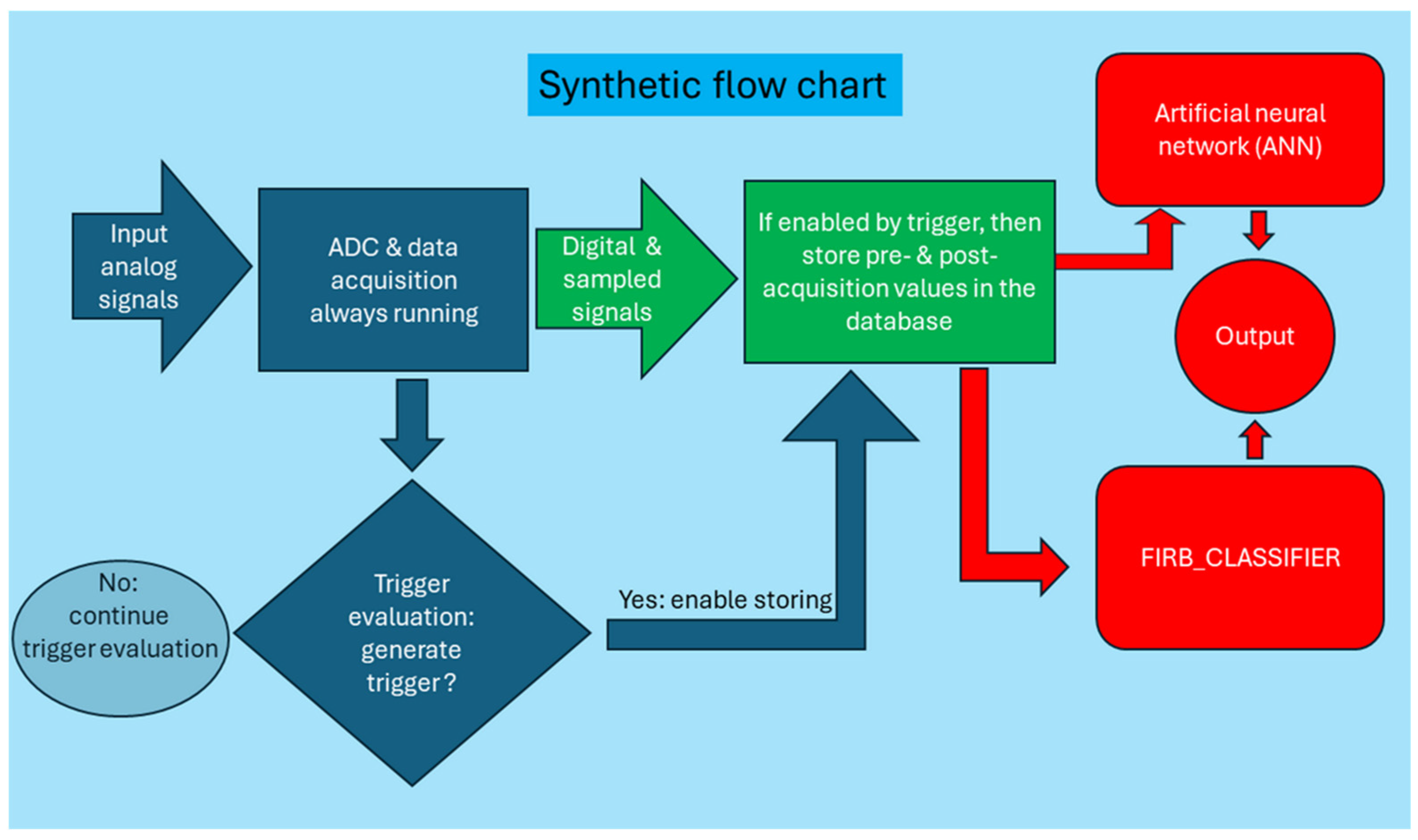
4.7. Flow Chart of the Software Modules

A summary of the concepts presented in this chapter is sketched in the flow chart in Figure 12, which includes all the modules discussed.

5. Discussion

5.1. The Project FAIRTEL

A new ultra-fast time-resolved mid-IR detection system for ground-based telescopes based on HgCdTe semiconductors has been proposed with the objective of searching for possible astronomical fast mid-infrared bursts (FIRBs). It is a directional instrument, and this feature can be useful for observations in areas of multi-messenger and time-domain astronomy.

The main elements of the instrument are as follows:

• A reflecting ground-based telescope (Cassegrain or Ritchey–Chrétien) with a main mirror and a minimum diameter of 400 mm, dedicated to the experiment for a long enough period of time.
• An infrared time-resolved detector comprising just one “A” astronomical pixel (or, as an alternative, seven “A” pixels in parallel) that is able to acquire fast signals with a rise time of the order of 1 ns, based on diagnostics developed for lepton storage rings; the detector will be put in the focal plane of the telescope to convert mid-IR light to electric analog signals. One “D” pixel (or, as an alternative, up to 12 pixels in parallel) are also foreseen for detecting background.
• Analog circuits (bias-tee, printed circuit board put in parallel 7 A + 12 D detectors and amplifiers with a gain of 80 dB) to adapt the analog signal to the digital acquisition system.
• A digital acquisition system sampling at least at 4 Gsamples/s and storing data when enabled by the trigger module; to have a good dynamic range, conversion from analog to digital using 12/14/16 bits is required.
• A module with different types of triggers generated automatically using a dedicated real-time module to record only interesting events without the need of operator intervention and to avoid overloading the database memory.
• Offline programs for data evaluation and classification by implementing pattern recognition (PR) capability from artificial intelligence (AI) techniques. This is to analyze and classify the records in the database. A program emulating the possible transients to test the classifier performance has been developed and used to generate a database of possible shapes of the fast infrared bursts. The FIRB classifier has been developed using an approach derived from beam diagnostics for fast instabilities in lepton storage rings. The transient classification is performed by displaying the signal shape in the time domain with first and second derivatives, as well as in the frequency domain, and measuring the growth rate and amplitude of transients.

Comments on each item are as follows.

Items 2 and 3 are the analog front end of the experiment and also the most critical points. They have been tested successfully using pulsed IR synchrotron light at the LNF of INFN. The most important result is in the statement that follows:

“Considering the realistic possibility, for the engineered system, to use an 80 dB amplification stage, that it is equivalent to a 10 k linear gain, the detection system shall be sensitive to one photon for 0.1% of the infrared bandwidth (δλ/λ) by using the needed 80 dB amplification.”

Items 1 and 4 require a high budget (and telescope usage time), but basically, they do not foresee demanding R&D activities.

The trigger module, in item 5, has been simulated using Octave programs. In the final version, the code should be rewritten using a faster programming language like C/C++ or, in the case of implementation for a FPGA, using VHDL or Verilog.

Item 6, offline post-processing software to emulate and to classify the astronomical infrared bursts, has been developed using procedural programming language (Octave). For the classifier, a possible alternative approach for implementing the pattern recognition module could be based on machine learning techniques and artificial neural networks. This approach is foreseen for in future development because it needs to collect a much larger database.

5.2. Toward a Feasibility Study

In summary, a preliminary design for a fast middle-infrared ground-based telescope, working to obtain time-domain signals, has been discussed, with an evaluation of performance. Note that other infrared telescopes, such as, for example, the JWST, work to obtain images and spectrographs, not ultra-fast time-domain signals. Photometry also requires signal integration. A comparison can be made with reference to fast time-domain detection systems in radio wave, visible, near-IR, gamma ray and gravitational wave observatories: detectors able to work in a time scale of 1 ns do not appear to be currently in progress.

The work conducted is a step toward a feasibility study. True astronomical tests should help provide more detail for the design. The objective is to place the mid-IR detector in the focal plane of a ground-based reflecting telescope, such as a Cassegrain or a Ritchey–Chrétien.

Alternatively, for observing low-frequency signals in the range between a few Hz and mHz, another technology, an InAsSb photovoltaic semiconductor by Hamamatsu, has been tested. It has a less performant rise time, around 20 ns, and it requires more gain, needing an amplification of at least 70 dB to observe a minimum useful signal. However, photovoltaic detectors can be used for low-frequency signals.

References

1. Lorimer, D.R.; Bailes, M.; McLaughlin, M.A.; Narkevic, D.J.; Crawford, F. A bright millisecond radio burst of extragalactic origin. Science 2007, 318, 777–780. [Google Scholar] [CrossRef] [PubMed]
2. Popov, S.B.; Postnov, K.A.; Pshirkov, M.S. Fast radio bursts. Physics-Uspekhi 2018, 61, 965. [Google Scholar] [CrossRef]
3. Hauser, M.G.; Dwek, E. The Cosmic Infrared Background: Measurements and Implications. Annu. Rev. Astron. Astrophys. 2001, 39, 249–307. [Google Scholar] [CrossRef]
4. Helou, G. The Interpretation of Modern Synthesis Observations of Spiral Galaxies; Duric, N., Crane, P.C., Eds.; Astronomical Society of the Pacific: San Francisco, CA, USA, 2001; Volume 275, pp. 125–133. [Google Scholar]
5. Platts, E. Computational Analysis Techniques Using Fast Radio Bursts to Probe Astrophysics. Ph.D. Thesis, University of Cape Town, Cape Town, South-Africa, 2012. Available online: http://hdl.handle.net/11427/33921 (accessed on 25 May 2024).
6. Petroff, E.; Hessels, J.W.T.; Lorimer, D.R. Fast radio bursts. Astron. Astrophys. Rev. 2019, 27, 4. [Google Scholar] [CrossRef]
7. Michilli, D.; Seymour, A.; Hessels, J.W.T.; Spitler, L.G.; Gajjar, V.; Archibald, A.M.; Bower, G.C.; Chatterjee, S.; Cordes, J.M.; Gourdji, K.; et al. An extreme magneto-ionic environment associated with the fast radio burst source FRB 121102. Nature 2018, 553, 182–185. [Google Scholar] [CrossRef] [PubMed]
8. Tendulkar, S.P.; Bassa, C.G.; Cordes, J.M.; Bower, G.C.; Law, C.J.; Chatterjee, S.; Adams, E.A.K.; Bogdanov, S.; Burke-Spolaor, S.; Butler, B.J.; et al. The host galaxy and redshift of the repeating fast radio burst FRB 121102. Astrophys. J. 2017, 834, L7. [Google Scholar] [CrossRef]
9. Rane, A.; Lorimer, D. Fast Radio Bursts. J. Astrophys. Astron. 2017, 38, 55. [Google Scholar] [CrossRef]
10. Scholz, P.; Bogdanov, S.; Hessels, J.W.; Lynch, R.S.; Spitler, L.G.; Bassa, C.G.; Bower, G.C.; Burke-Spolaor, S.; Butler, B.J.; Chatterjee, S.; et al. Simultaneous X-ray, gamma-ray, and radio observations of the repeating fast radio burst FRB 121102. Astrophys. J. 2017, 846, 80. [Google Scholar] [CrossRef]
11. Hardy, L.K.; Dhillon, V.S.; Spitler, L.G.; Littlefair, S.P.; Ashley, R.P.; De Cia, A.; Green, M.J.; Jaroenjittichai, P.; Keane, E.F.; Kerry, P.; et al. A search for optical bursts from the repeating fast radio burst FRB 121102. Mon. Not. R. Astron. Soc. 2017, 472, 2800–2807. [Google Scholar] [CrossRef]
12. Farah, W.; Flynn, C.; Bailes, M.; Jameson, A.; Bannister, K.W.; Barr, E.D.; Bateman, T.; Bhandari, S.; Caleb, M.; Campbell-Wilson, D.; et al. FRB microstructure revealed by the real-time detection of FRB170827. Mon. Not. R. Astron. Soc. 2018, 478, 1209–1217. [Google Scholar] [CrossRef]
13. Burgay, M. Fast Radio Bursts-Mysterious Probes of the Universe. In Proceedings of the Talk for the GSSI Astroparticle Colloquia, L’Aquila, Italy, 18 November 2020. [Google Scholar]
14. Haggard, H.M.; Rovelli, C. Black Hole Fireworks: Quantum-gravity Effects Outside the Horizon Spark Black to White Tunnelling. Phys. Rev. D 2015, 92, 104020. [Google Scholar] [CrossRef]
15. Barrau, A.; Rovelli, C.; Vidotto, F. Fast radio bursts and white hole signals. Phys. Rev. D 2014, 90, 127503. [Google Scholar] [CrossRef]
16. Rovelli, C. (Aix Marseille Universite, CNRS, Marseille, France). Personal communication, 2024.
17. Rovelli, C. Relatività Generale; (It. tr. Pietropaolo Frisoni from General Relativity); Adelphi Edizioni: Milano, Italy, 2021; p. 163. ISBN 978-88-459-3608-1. [Google Scholar]
18. Rovelli, C. Buchi Bianchi; Adelphi Edizioni: Milano, Italy, 2023; p. 144. ISBN 978-88-459-3753-8. [Google Scholar]
19. Drago, A.; Bini, S.; Guidi, M.C.; Marcelli, A.; Bocci, V.; Pace, E. A Proposal for a Fast Infrared Bursts Detector. J. Instrum. 2024, 19, P05027. [Google Scholar] [CrossRef]
20. Chen, Y.; Sun, X.; Li, Z.; Wang, C.; Zhang, C.; Sun, S. Detection system of the lobster eye telescope with large field of view. Appl. Opt. 2022, 61, 8813–8818. [Google Scholar] [CrossRef]
21. Abbott, B.; Abbott, R.; Abbott, T.D.; Abernathy, M.R.; Acernese, F.; Ackley, K.; Adams, C.; Adams, T.; Addesso, P.; Adhikari, R.X.; et al. (LIGO Scientific Collaboration and Virgo Collaboration). Observation of Gravitational Waves from a Binary Black Hole Merger. Phys. Rev. Lett. 2016, 116, 061102. [Google Scholar] [CrossRef]
22. Branchesi, M.; Maggiore, M.; Alonso, D.; Badger, C.; Banerjee, B.; Beirnaert, F.; Belgacem, E.; Bhagwat, S.; Boileau, G.; Borhanian, S.; et al. Science with the Einstein Telescope: A comparison of different designs. J. Cosmol. Astropart. Phys. 2023, 2023, 68. [Google Scholar] [CrossRef]
23. Sands, M. The Physics of Electron Storage Rings: An Introduction; Technical Rep. SLAC-R-121; SLAC: Stanford, CA, USA, 1970. [Google Scholar]
24. Chao, A.W.; Tigner, M. Handbook of Accelerator Physics and Engineering; World Scientific Publishing, Co.: Singapore, 1999; ISBN 9810235003. [Google Scholar]
25. De Santis, A.; Alesini, D.; Behtouei, M.; Bilanishvili, S.; Bini, S.; Boscolo, M.; Buonomo, B.; Cantarella, S.; Cardelli, F.; Ciarma, A.; et al. DaΦne Run for the Siddharta-2 Experiment. In Proceedings of the IPAC’23, 14th International Particle Accelerator Conference, Venice, Italy, 7–12 May 2023; Available online: https://accelconf.web.cern.ch/ipac2023/pdf/MOPL085.pdf (accessed on 7 May 2025).
26. INFN, Laboratori Nazionali di Frascati. DAΦNE-LIGHT Synchrotron Radiation Facility. Available online: http://dafne-light.lnf.infn.it/ (accessed on 1 September 2024).
27. Guidi, M.C.; Piccinini, M.; Marcelli, A.; Nucara, A.; Calvani, P.; Burattini, E. Optical performances of SINBAD, the Synchrotron Infrared Beamline At DAΦNE. J. Opt. Soc. Am. A 2005, 22, 2810–2817. [Google Scholar] [CrossRef]
28. Prabhakar, S. New Diagnostics and Cures for Coupled-Bunch Instabilities. Ph.D. Thesis, Stanford University, Stanford, CA, USA, 2000. [Google Scholar]
29. Laclare, J.L. Bunched beam instabilities. In Proceedings of the High Energy Accelerators, Geneva, Switzerland, 7–11 July 1980; Birkhauser: Basel, Switzerland, 1980; pp. 526–539. [Google Scholar]
30. Drago, A.; Raimondi, P.; Zobov, M.; Shatilov, D. Synchrotron oscillation damping by beam-beam collisions in DAΦNE. Phys. Rev. ST Accel. Beams 2011, 14, 092803. [Google Scholar] [CrossRef]
31. Migliorati, M.; Palumbo, L.; Zannini, C.; Biancacci, N.; Vaccaro, V.G. Resistive wall impedance in elliptical multilayer vacuum 1607 chambers. Phys. Rev. Accel. Beams 2019, 22, 121001. [Google Scholar] [CrossRef]
32. Migliorati, M.; Antuono, C.; Carideo, E.; Zhang, Y.; Zobov, M. Impedance modelling and collective effects in the Future Circular e+e- Collider with 4 IPs. Eur. Phys. J. Tech. Instrum. 2022, 9, 10. [Google Scholar] [CrossRef]
33. Piotrowski, J.; Rogalski, A. Uncooled long wavelength infrared photon detectors. Infrared Phys. Technol. 2004, 46, 115–131. [Google Scholar] [CrossRef]
34. Piotrowski, A.; Madejczyk, P.; Gawron, W.; Kłos, K.; Pawluczyk, J.; Rutkowski, J.; Piotrowski, J.; Rogalski, A. Progress in MOCVD growth of HgCdTe heterostructures for uncooled infrared photodetectors. Infrared Phys. Technol. 2007, 53, 2. [Google Scholar] [CrossRef]
35. Piotrowski, J.; Pawluczyk, J.; Piotrowski, A.; Gawron, W.; Romanis, M.; Kłos, K. Uncooled MWIR and LWIR photodetectors in Poland. Opto-Electron. Rev. 2010, 18, 318–327. [Google Scholar] [CrossRef]
36. Bocci, A.; Marcelli, A.; Pace, E.; Drago, A.; Piccinini, M.; Guidi, M.C.; De Sio, A.; Sali, D.; Morini, P.; Piotrowski, J. Fast Infrared Detectors for Beam Diagnostics with Synchrotron Radiation. Nucl. Instrum. Methods Phys. Res. Sect. A 2007, 580, 190–193. [Google Scholar] [CrossRef]
37. Drago, A.; Bocci, A.; Cestelli Guidi, M.; De Sio, A.; Pace, E.; Marcelli, A. Bunch-by-bunch profile diagnostics in storage rings by infrared array detection. Meas. Sci. Technol. 2015, 26, 094003. [Google Scholar] [CrossRef]
38. Drago, A.; Bini, S.; Guidi, M.C.; Marcelli, A.; Pace, E. Fast Rise Time IR Detectors for Lepton Colliders. J. Instrum. 2016, 11, C07004. [Google Scholar] [CrossRef]
39. VIGO Photonics. Available online: https://vigophotonics.com/app/uploads/2022/06/VIGO_katalog_2020-2021-LQ-1.pdf (accessed on 23 September 2021).
40. Hamamatsu Photonics. Available online: https://www.hamamatsu.com/eu/en.html (accessed on 30 January 2023).
41. Drago, A.; Pace, E.; Bini, S.; Guidi, M.C.; Curceanu, C.; Marcelli, A.; Bocci, V. Ultra-Fast Infrared Detector for Astronomy. Nucl. Instrum. Methods Phys. Res. A 2023, 1048, 167936. [Google Scholar] [CrossRef]
42. Drago, A.; Pace, E.; Bini, S.; Guidi, M.; Cioeta, F.; Marcelli, A.; Bocci, V. Fast Transient Infrared Detection for Time-domain Astronomy. J. Instrum. 2023, 18, C02012. [Google Scholar] [CrossRef]
43. Drago, A.; Pace, E.; Bini, S.; Guidi, M.C.; Cioeta, F.; Marcelli, A.; Bocci, V. Performance evaluation of an Ultra-Fast IR Detector for Astronomy Transients. J. Phys. Conf. Ser. 2023, 2579, 012013. [Google Scholar] [CrossRef]
44. Teledyne ADQ7DC-10 GSPS, 14-bit Digitizer. Available online: https://www.spdevices.com/what-we-do/products/hardware/14-bit-digitizers/adq7dc (accessed on 7 May 2025).
45. Octave GNU Octave, version 8.4.0. (2023-11-05). Copyright (C) 1993-2023 The Octave Project Developers. This Is Free Software. Available online: https://octave.org/ (accessed on 5 November 2023).
46. Available online: https://mathworks.com/ (accessed on 7 May 2025).
47. Bissaldi, E. Multi-messenger studies with the Fermi Satellite. In Proceedings of the Neutrino Oscillation Workshop 2018, NOW2018, Rosa Marina, Ostuni, Italy, 9–16 September 2018; Available online: https://home.ba.infn.it/~now/now2018/assets/bissaldi_now2018.pdf (accessed on 12 February 2024).
48. Tou, J.T.; Gonzales, R.C. Pattern Recognition Principles; Addison-Wesley Publishing Company: Reading, MA, USA, 1974. [Google Scholar]
49. Cover, T.M.; Diday, E.; Rosenfeld, A.; Simon, J.C.; Wagner, T.J.; Weszka, J.S.; Wolf, J.J. Digital Pattern Recognition; Springer: Berlin/Heidelberg, Germany; New York, NY, USA, 1976. [Google Scholar]
50. Chen, C.H. Statistical Pattern Recognition; Hayden Book Company: Washington, DC, USA, 1973. [Google Scholar]
51. Andrews, H.C. Introduction to Mathematical Techniques in Pattern Recognition; Wiley: New York, NY, USA, 1972. [Google Scholar]
52. Drago, A. Elaborazione e Messa a Punto di un Procedimento per L’analisi Automatica di Strisce Elettroforetiche di Lipoproteine. Bachelor’s Thesis, Università di Roma (La Sapienza), Roma, Italy, 1978; pp. 174–IV. [Google Scholar]
53. Hopfield, J.J. Neural networks and physical systems with emergent collective computational abilities. Proc. Natl. Acad. Sci. USA 1982, 79, 2554–2558. [Google Scholar] [CrossRef]
54. Hinton, G.E. 6: How Neural Networks Learn from Experience. In Cognitive Modeling; Book Chapter; Polk, T., Seifert, C., Eds.; The MIT Press: Cambridge, MA, USA, 2002; ISBN 9780262281744. [Google Scholar] [CrossRef]
55. LeCun, Y.; Bengio, Y.; Hinton, G. Deep learning. Nature 2015, 521, 436–444. Available online: https://www.nature.com/articles/nature14539 (accessed on 2 May 2024). [CrossRef] [PubMed]
56. Goodfellow, I.; Bengio, Y.; Courville, A. Deep Learning; MIT Press: Cambridge, MA, USA, 2016; p. 800. ISBN 978-0262035613. [Google Scholar]
57. Soo, J.Y.H.; Shuaili, I.Y.K.; Pathi, I.M. Machine learning applications in astrophysics: Photometric redshift estimation. AIP Conf. Proc. 2023, 2756, 040001. [Google Scholar] [CrossRef]
58. Ciacci, G.; Barucci, A.; Di Ruzza, S.; Alessi, E.M. Asteroids co-orbital motion classification based on Machine Learning. Mon. Not. R. Astron. Soc. 2024, 527, 6439–6454. [Google Scholar] [CrossRef]
Figure 2. For astronomical observations in the infrared range, current telescopes cannot observe transients with a duration shorter than milliseconds.
Instruments 09 00012 g002
Figure 3. Positron (red) and electron (blue) longitudinal amplitude detection of 110 bunches in the time domain from two electromagnetic pickups connected directly to the oscilloscope and showing the separation of the bunches. The horizontal time scale is 30 ns per square.
Instruments 09 00012 g003
Figure 4. Spectral response detectivity D* of PC10.6 photoconductor. Data sheet sent by VIGO in attachment to the component.
Instruments 09 00012 g004
Figure 5. Amplified MCT detector signal (cyan trace; 2 mV per division), that reproduces the bunch train corresponding to the signal from the electromagnetic pickup (yellow trace of the oscilloscope). The red trace shows the machine master clock used as a trigger for the oscilloscope.
Instruments 09 00012 g005
Figure 6. The photovoltaic detector acquiring the synchrotron light (cyan trace; 2 mV per division). Red—the machine master clock; yellow—the beam signal coming from an electromagnetic pickup. Note that the difference in phase between the signals is not significant because the signals travel different paths.
Instruments 09 00012 g006
Figure 7. Fast IR burst emulation: several cases of data files created with or without noise: in the vertical axis, the amplitude in mV, in the horizontal axis, the number of acquired samples.
Instruments 09 00012 g007
Figure 8. From the analysis of data file 2024-7-31-17-44-48.txt: the classifier-plotted time-domain behavior (left/up), first derivative (right/up), second derivative (left/mid), absolute amplitude in the frequency domain after a Fast Fourier Transform (right/mid), real amplitude in the frequency domain after FFT (left/down) and imaginary amplitude in the frequency domain after a FFT (right/down).
Instruments 09 00012 g008
Figure 9. From the analysis of data file 2024-7-31-13-13-20.txt: the classifier-plotted time-domain behavior (left/up), first derivative (right/up), second derivative (left/mid), absolute amplitude in the frequency domain after a Fast Fourier Transform (right/mid), real amplitude in the frequency domain after a FFT (left/down) and imaginary amplitude in frequency domain after a FFT (right/down).
Instruments 09 00012 g009
Figure 10. From the analysis of data file 2024-7-31-18-0-36.txt: the classifier-plotted time domain behavior (left/up), first derivative (right/up), second derivative (left/mid), absolute amplitude in frequency domain after Fast Fourier Transform (right/mid), real amplitude in frequency domain after FFT (left/down), imaginary amplitude in frequency domain after FFT (right/down).
Instruments 09 00012 g010
Figure 11. From the analysis of data file 2024-7-31-18-15-49.txt: the classifier-plotted time-domain behavior (left/up), first derivative (right/up), second derivative (left/mid), absolute amplitude in the frequency domain after a Fast Fourier Transform (right/mid), real amplitude in the frequency domain after a FFT (left/down) and imaginary amplitude in frequency domain after a FFT (right/down).
Instruments 09 00012 g011
Figure 12. Flow chart summarizing the modules discussed. The implementation of noise-canceling filters is included inside the two red blocks (firb_classifier and ANN).
Instruments 09 00012 g012
Disclaimer/Publisher’s Note: The statements, opinions and data contained in all publications are solely those of the individual author(s) and contributor(s) and not of MDPI and/or the editor(s). MDPI and/or the editor(s) disclaim responsibility for any injury to people or property resulting from any ideas, methods, instructions or products referred to in the content.