Article

Metrological-Characteristics-Based Calibration of Optical Areal Surface Measuring Instruments and Evaluation of Measurement Uncertainty for Surface Texture Measurements

Physikalisch-Technische Bundesanstalt, Bundesallee 100, 38116 Braunschweig, Germany
*
Author to whom correspondence should be addressed.
Instruments 2025, 9(2), 11; https://doi.org/10.3390/instruments9020011
Submission received: 27 February 2025 / Revised: 30 April 2025 / Accepted: 1 May 2025 / Published: 8 May 2025

Abstract

:
ISO 25178 part 600:2019 and part 700:2022 introduce a calibration framework based on seven metrological characteristics (MCs) for calibrating optical areal surface measuring instruments. Among these, topography fidelity is a newly defined metrological characteristic that remains a critical yet unresolved challenge in instrument calibration. This paper proposes strategies to address topography fidelity, including a key criterion for selecting suitable instrument setups by comparing slope measurement capability with local surface slopes, as well as methods for investigating the field-of-view homogeneity and directional performance difference along the x- and y-axes. Furthermore, the uncertainty contribution of topography fidelity in surface topography measurements is analysed. The paper also determines the uncertainty associated with the remaining six MCs. Based on the proposed MC-based calibration approach and the corresponding uncertainty contributions, an overall measurement uncertainty model for Sa and Sq parameters is presented. Finally, uncertainty evaluations for Sa and Sq are demonstrated on a challenging surface, where topography fidelity plays a significant role in the measurement uncertainty evaluation.

1. Introduction

Surface texture measurements are critical in a wide range of industrial applications, as they are needed to determine the functional properties of surfaces, such as friction [1,2], wear [3], and adhesion [4]. Various factors, including instrument calibration, measurement setup, environmental conditions, and the surface characteristics, influence measurement uncertainty, thereby affecting the precision and reliability of these measurements.
Optical topography measuring instruments including coherence scanning interferometry (CSI) [5], confocal microscopy (CM) [6], and focus variation instruments (FV) [7] are increasingly used for surface texture measurements due to their advantages of being fast and non-contact. However, each type of instrument has its own measurement principle, hardware configuration, and microscope objectives with varying numerical apertures. Additionally, the complex interaction between light and intricate surface textures further complicates the selection of appropriate optical instruments, their setup, and the evaluation of measurement uncertainty.
Although measurement uncertainty is highly significant, a universally accepted approach for determining the measurement uncertainty of optical surface topography instruments has yet to be developed and remains an active area of research.
The ISO 25178 standard series—Geometrical product specifications (GPS)—Surface texture: Areal—provides a comprehensive framework for the calibration of surface topography measuring instruments. Specifically, ISO 25178 Part 600: 2019 [8] defines the key metrological characteristics (MCs) of instruments, while Part 700: 2022 [9] describes the methods and material measures used to characterize these key metrological characteristics for the calibration of optical surface texture measuring instruments. Together, these standards form the foundation for evaluating instrument performance and understanding the impact of metrological characteristics on measurement results.
However, these standards do not provide a model for evaluating the overall measurement uncertainty. In particular, due to the complex interaction between light and surface, no default method or material measure is specified for calibrating the newly defined MC of topography fidelity.
Efforts to evaluate the measurement uncertainty—such as good practice guides developed at NPL [10,11] and refs. [12,13,14,15,16]—do not account for topography fidelity. Furthermore, the uncertainty contributions of some MCs are mixed together, making it difficult to distinguish the individual effects. In refs. [17,18] stylus reference measurements were conducted to determine topography fidelity. However, performing stylus measurements over the same field of view (FOV) as optical measurements—such as the 258 µm × 258 µm FOV of a 50× objective—is highly time-consuming. Additionally, topography fidelity is object-dependent, meaning that for complex surfaces, optical measurements must always be validated by comparing the entire FOV area with reference measurements.
A well-distinguished uncertainty contribution for each MC, a well-defined measurement strategy, and clear criteria for evaluating topography fidelity are urgently needed to improve uncertainty evaluation in surface texture measurements using optical instruments.
In this paper, Section 2 introduces the metrological characteristics of areal surface measuring instruments as defined in ISO 25178-600 [8]. Section 3 describes the methods and material measures used for calibrating MCs, with a focus on determining the uncertainty of each MC, particularly topography fidelity. Section 4 presents a general measurement uncertainty model for height parameters of surface texture (i.e., Sa and Sq) and provides an example of uncertainty determination for Sa and Sq on a highly challenging surface, where topography fidelity plays a significant role in the measurement uncertainty evaluation.

2. Metrological Characteristics for Optical Areal Surface Measuring Instruments

A metrological characteristic is defined in ISO 25178-600:2019 [8] as a characteristic of measuring equipment that can influence measurement results. Table 1 lists the MCs for surface measurement methods defined in ISO 25178-600:2019.
The metrological characteristics are designed to capture all factors that can influence a measurement result (influence quantities) and can be propagated appropriately through a specific measurement model to evaluate measurement uncertainty. The calibration of an instrument’s metrological characteristics enables the comparison of systems based on different measurement principles or different configurations.
The following similarity conditions should be applied when calibrating the MCs [9]:
(1)
The instrument setup (configuration) and environmental conditions should be similar to those during the actual measurement activity for that instrument.
(2)
Calibration should be performed within the same measurement volume defined for the intended application.
(3)
In applications where filters or operators are used, the flatness determination should proceed under the same filter conditions as those used for measurements.
It should be noted that in this paper, the uncertainty caused by filters, software, and algorithms used for parameter calculation are not taken into account.

3. Determination of the MCs and the Corresponding Measurement Uncertainty Contributions for Surface Texture Measurements

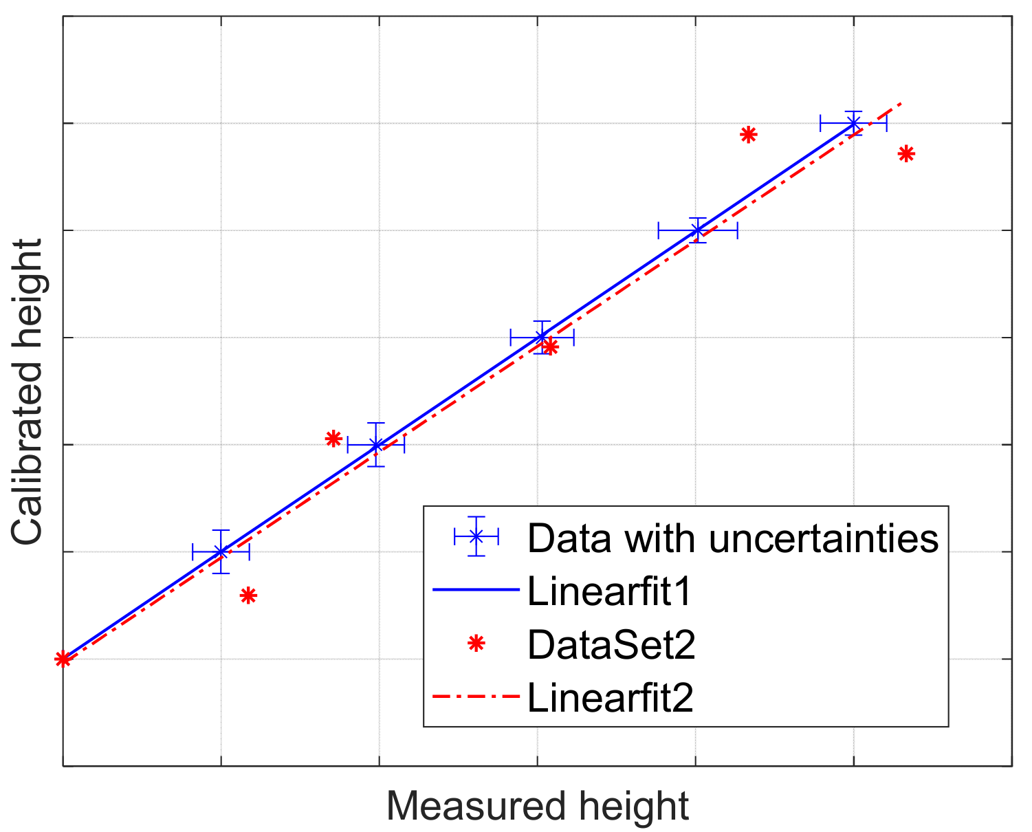
3.1. Amplification Coefficient

Amplification coefficients ( α x , α y , α z ) are defined in ISO 25178-600 as the slope of the linear regression line obtained from the response function.
For the z-axis, this is done by comparing the measured depth with the calibrated depth of the step height or depth. The amplification coefficient is determined from the quotient of the calibrated depth dcal (numerator) and the measured depth value d m e a s (denominator), i.e., d c a l d m e a s [9].
Single step material measures might be sufficient for some given applications, for example, maximum height (Sz) or step height (d) measurements. In this case, the amplification coefficient of the z-axis can be expressed as follows:
α z = d c a l d m e a s
According to GUM [19], the combined standard uncertainty of a function f of variables x i is given by Equation (2) for propagation of uncertainty:
u f 2 = i = 1 N f x i 2 u 2 x i
Thus, the combined standard uncertainty of α z then can be determined by the following:
u 2 α z = 1 d m e a s 2 u d c a l 2 + 1 n · d c a l d m e a s 2 2 u d m e a s 2 1 d m e a s 2 u d c a l 2 + 1 n · u d m e a s 2
in which d c a l is the calibrated value of height, d m e a s is the measured value of height, u d c a l is the standard uncertainty of the calibrated height, and u d m e a s is the standard deviation of measured height determined by n-times repeated measurements.
However, for the determination of texture parameters, several step-heights should be used, and the step heights to be measured should be within the same z-range of the measurement application. In this case, the amplification coefficient is determined by fitting a line to the determined step depths or step heights using the least-squares method [9].
As already used in Equation (3), each step height has a calibrated value with a standard uncertainty u d c a l , and a measured height which is normally a mean value with a standard deviation u d m e a s by averaging some repeated measurements. The uncertainties in the calibrated and measured heights for linear fitting need to be accounted for. As illustrated in Figure 1, different fitting lines, corresponding to different slopes, will be obtained by randomly choosing different datasets in the corresponding uncertainty ranges. Therefore, the combined standard uncertainty of αz consists of two parts: one is the standard uncertainty of the slope determined by linear fitting itself, while the other one is the standard deviation of the slopes caused by the uncertainty of the calibrated and measured heights.
The former (linear fitting standard uncertainty) is determined by dividing the standard deviation of the residuals by the height range used for the linear fitting.
The latter is determined by a Monte-Carlo simulation [20] in this paper with sufficient N (e.g., 10,000) times randomly selected datasets, i.e., calibrated and measured height values within their respective standard deviation specified intervals (both normal distributions). An algorithm developed in ref. [21] for fitting a straight line to data with uncertainties in both coordinates can also be used for the determination of this standard uncertainty.
Finally, the uncertainty contribution to the overall measurement uncertainty caused by the amplification coefficient αz can be determined by the following:
u α z = u α z · z
Amplification coefficients of the x- and y-axis can be determined using a cross grating (s. detailed procedure in ISO 25178-700 [9]). The corresponding combined standard uncertainty can be similarly determined.

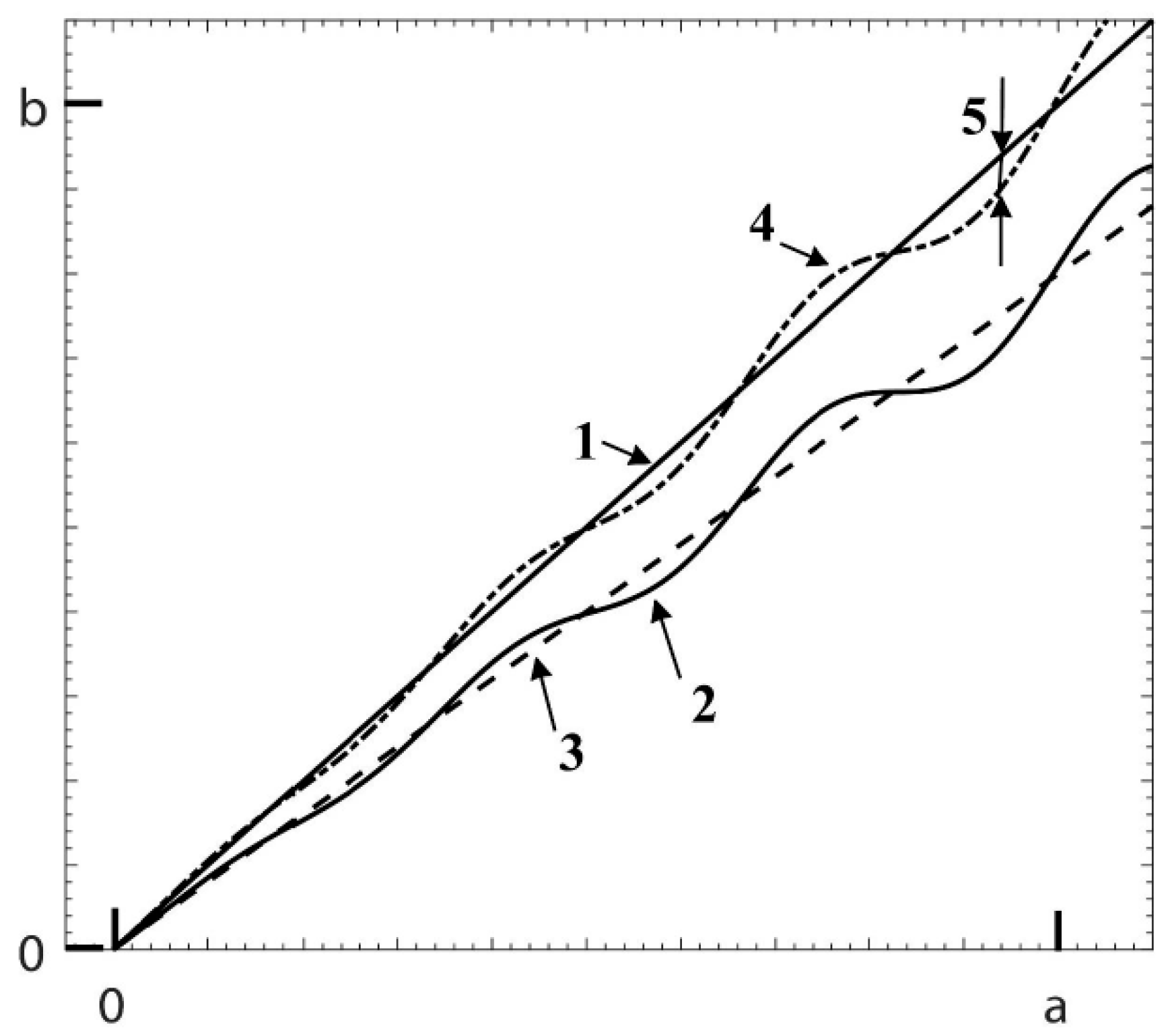
3.2. Linearity Deviation

The linearity deviations l x , l y , l z are defined in ISO 25178-600 [8] as the maximum local difference between the line from which the amplification coefficient is derived and the response function.
The linearity deviation lz is determined from the same measurements with step heights for determination of the amplification coefficient.
It should be noted that the assessed parameter l z is the maximum deviation of measured heights/depths dmeas to the calibrated heights/depths dcal after adjustment of the amplification coefficient α z (see Figure 2, key 5 and 3.1.11 in ref. [9]).
In addition, ref. [22] proposed a relatively simple procedure for a long z-axis range if a material measure with several negative (grooved) steps, which do not share a common reference plane, is used and stitches together to determine the amplification coefficient and linearity deviation.
Finally, the measurement uncertainty contribution ulz to the overall measurement uncertainty caused by linearity deviation ± l z is propagated in the form of a rectangular distribution which has a variance of 2 · l z 2 / 12 [19]. Therefore, we obtain the following:
u l z = l z 3
Linearity deviations of the x- and y-axis can be determined using a cross grating (s. detailed procedure in ref. [9]). The corresponding combined standard uncertainty can be similarly determined.

3.3. Flatness Deviation

Flatness deviation zFLT is the deviation of the measured topography of an ideally flat object from a plane [8]. The default material measure for the determination of the flatness deviation is a flat measurement standard, preferably an optically smooth standard. The assessed parameter for flatness deviation zFLT is Sz as defined in ISO 25178-2:2012 [23].
The effect of the optical flat itself and the effect of the instrument noise can be reduced by measuring different areas on the optical flat and averaging the topography values [9,24,25].
The way to estimate the residual flatness described in ref. [9] is to measure the flat at different locations and to average the height measurement at each location. The contribution of the flat and any spurious data should diminish whereas the quality of the areal reference should be preserved [17]. However, in practice, it is difficult to recommend how many repeated measurements need to be performed to separate the flatness deviation of the instrument from that of the contribution of flat and other spurious measurement data. To address this problem, a threshold method is proposed and detailed in ref. [12] which can be easily applied by using a high-order polynomial to remove the form and thresholding the peaks and valleys of the residual surface larger than three times the Sq value of the residual surface.
The uncertainty distribution of the residual flatness is complicated. In ref. [14], it is assumed that the residual flatness is more like a bimodal distribution, while in ref. [17], the residual flatness contribution is propagated in the form of a rectangular distribution. Since both distributions essentially provide very similar values for the uncertainty contribution, we will use the latter for the calculation, i.e., the residual flatness u F L T to the overall measurement uncertainty has a variance of z F L T 2 / 12 [19]. Therefore, we obtain the following:
u F L T = z F L T 2 3

3.4. Measurement Noise

Measurement noise (NM) is the noise added to the output signal occurring during the normal use of the instrument [8].
The default method to estimate the measurement noise is the subtraction method: An optical flat is measured twice at the same location with the shortest possible time difference between the two sequential measurements. The two measured topographies are subtracted from each other. The RMS value is calculated on the difference topography without any filter giving Sq.
The measurement noise is determined as N M = S q / 2 [9]. The division by √2 accounts for the fact that each of the two measurements contributes to the noise.
u N o i s e = N m
For alternative methods of estimation of measurement noise by the averaging method or determination of the stabilized measurement noise, see also 6.5.4.4 and 6.5.4.5 in ref. [9].

3.5. x, y-Mapping Deviations

The mapping deviations x x , y   and y x , y of the instrument’s x- and y-axis are defined in ISO 25178-600:2019 as a gridded image of x- and y-deviations of actual coordinate positions on a surface from their nominal positions.
Grid-type material measures (areal cross gratings) with calibrated distances in the x-y plane can be used as default material measure for the determination of the mapping deviations of the x and y axis. The detailed description of the procedure can be seen in ref. [9].
As the main potential errors of mapping deviations are in the x- and y-directions, the contribution of the mapping deviations to the overall measurement uncertainty can be negligible, depending on the parameter considered, for example, a step height or the Sa parameter [9]. In this paper, we aim to develop a model for the measurement uncertainty of height parameters such as Sa and Sq. The contribution of mapping deviations to other parameters, such as spatial and hybrid parameters, is beyond the scope of this paper.

3.6. Topographic Spatial Resolution

Topographic spatial resolution is defined in ISO 25178-600 as the metrological characteristic describing the ability of a surface topography measuring instrument to distinguish closely spaced surface features. Several parameters have been defined to actually quantify the topographic spatial resolution, depending on the application and the method of measurement, such as the lateral period limit DLIM [8,26,27,28], the width limit for full height transmission Wl [8,29,30], the small scale fidelity limit TFIL [8,31,32], the Rayleigh criterion, and the Abbe resolution limit [8].
In the EU project TracOptic [33] the width limit for full height transmission Wl has been investigated to determine the topographic spatial resolution. Wl is defined as the width of the narrowest rectangular groove whose step height is measured within a given tolerance [8]. In ref. [30] a robust algorithm to determine the pitch and height of 1D grating measurement standards was developed and 1D gratings with different heights and pitches were measured and evaluated. Figure 3 shows one measurement result of a RS-N [34] 1D grating measured by a confocal laser scanning microscope with 20×, 50×, and 100× objectives, respectively. The RS-N consists of 1D gratings with a nominal height of 0.19 µm and pitches of 0.3 µm, 0.4 µm, 0.6 µm, 0.8 µm, 1.2 µm, 2.0 µm, 3.0 µm, 4.0 µm, and 6.0 µm. Two tolerances, 5% and 10% of the reference height of the grating, were specified for Wl evaluation according to ISO 25178-600:2019. It can be seen that the 20× objective could not measure the height within a 10% tolerance, while the 50× and 100× objectives can measure the height of structures with a width of 1.4 µm and 0.5 µm within 10% tolerance, respectively. One more step should be carried out, namely testing different heights with the same pitch series or pitch range to investigate whether the Wl is a height-dependent parameter. However, no appropriate material measures were available for this investigation in the runtime of TracOptic. Therefore, suitable material measures—rectangular shape gratings for Wl investigation or sinusoidal shape gratings for DLIM investigation, with sufficient pitches (200 nm to 20 μm) and varying amplitudes (from submicron to several micrometres) for different objectives of optical topography measuring instruments—need to be urgently developed.
As listed in Table 1, the topographic spatial resolution can introduce potential errors in the z-direction if the surface texture features are not correctly resolved. We assume that, for surface texture measurements, if the autocorrelation length of the surface is larger than the topographic spatial resolution, for example Wl, the uncertainty contribution u r e s o l u t i o n to the overall measurement uncertainty can be neglected. To assure this, the topographic spatial resolution Wl should be determined with a 1D grating whose height is comparable to the height values of the surface texture, such as Sa or Sq. Therefore, for a specific surface texture, some prior knowledge—such as the height and the autocorrelation length—are required to select an appropriate objective for measuring the surface texture with low uncertainty.

3.7. Topography Fidelity

Topography fidelity TFI is defined as the closeness of agreement between a measured surface profile or measured topography and one whose uncertainties are insignificant by comparison [8]. The topography fidelity accounts for all remaining effects where the other six metrological characteristics have been evaluated and accounted for. The topography fidelity depends on influence quantities that can include surface slopes and discontinuous features (sharp edges) as well as the specimen properties such as refractive index, reflectivity, and the presence of transparent thin films, the elastic modulus, or hardness [9].
There are no standard material measures and methods for determining the topography fidelity defined in ISO 25178-700:2022 [9]. Acceptable methods include comparison with reference metrology, the use of reproducibility tests with variations in part orientation between measurements, experimental methods to determine sensitivities of the measured results to changes in the instrument configuration, and the use of virtual instruments [9,35,36]. In recent years, some materials measures [37,38], such as rectangular chirp structures [39] and sinusoidal chirp structures [40,41,42,43], have been developed and corresponding experimental [31,32,44] and modelling [35,45,46,47,48,49] methods to investigate the topography fidelity have been reported. However, it is not clear how the results can be incorporated into the measurement uncertainty budget for specific surface texture measurement tasks.
To address the topography fidelity issue, strategies have been developed. The following steps are proposed to evaluate the measurement uncertainty:
Step (1): Selection of an appropriate microscope objective to minimize the measurement artefacts, such as overshooting, multireflection, and so on, caused by surface local slopes: The maximum measurable slope of the used objective should be large enough to measure the local slopes of the surface. In the recently developed Good Practice Guide on the selection of instrumentation for optical roughness measurements with confocal microscopes (CM), coherence scanning interference microscopes (CSI) and focus variation instruments (FV) [50], a key criterion is set for the selection of the microscope objective, namely θ N A > θ 95 % . θ N A is the maximum measurable slope of the objective with a numerical aperture of NA. It can be determined by using a sinusoidal chirp standard developed at PTB with largest slope of about 40° [43] or other material measures such as spheres [51]; if both methods are not available, the theoretical value of θ N A = arcsin ( N A )   can be used for estimation. θ 95 % is the slope threshold, corresponding to the 95th percentile of the slope distribution of the surface to be measured—that is, 95% of the local slope values are less than or equal to this threshold [50]. To calculate the slope threshold θ 95 % of a surface, a reference measurement with sufficient lateral resolution—or an optical measurement ideally performed with a significantly higher numerical aperture, ensuring that θ N A θ 95 % and delivering high measurement performance—is required. Figure 4 illustrates an example of how to determine the θ 95 % using a measured topography image. Figure 4a shows a cropped topography image of the central 90 µm × 90 µm area, measured using a confocal laser scanning microscope (CLSM) with a 50× objective (NA = 0.95). Figure 4b presents the corresponding slope distribution of the measured surface, along with the slope threshold θ 95 % . The local slope angle θ at each point i in the topography image is calculated according to ISO 25178-2: Annex D.1 Local gradient vector [23]. Based on the calculated local slope angles, the probability density (in %) as a function of the slope angle is then determined. By selecting a microscope objective that is able to measure these slopes, the uncertainty contribution u s l o p e caused by large local slopes to the overall measurement uncertainty can also be neglected.
Step (2): Investigate the different image quality (inhomogeneity) within the FOV of the used objective: We found that in some cases, even when the condition θ N A > θ 95 % is satisfied, especially for surfaces with a larger θ 95 % —value (for example θ 95 % > 40 ° ), the image quality within the FOV of the used objective becomes different when measuring with a laser scanning confocal microscope using, for example, a 50× objective with a numerical aperture of 0.95. The inhomogeneity of the FOV, in this context, refers to whether the same quality of the topography images can be obtained when the same surface area is measured in the different positions within the FOV. The inhomogeneity of the FOV is both object- and measurement-principle-dependent and therefore needs to be investigated. In ref. [52], we proposed a simple experimental method to investigate the inhomogeneity of the FOV for a specific surface area by moving the area to different positions within the FOV and comparing the resulting roughness parameters, and various surfaces with different θ 95 % values, each smaller than θ N A , were measured using a laser scanning confocal microscope, and a thorough analysis was conducted to assess the robustness and applicability of the proposed method. Reference measurement of the test region of the surface should be performed to validate the optical measurement. The topography fidelity of the test region u f i _ r e f can be estimated by calculating the difference between the reference and the optical measurements in the test region. If the optical measurement shows larger deviations from the reference measurement, an objective with a larger NA in step (1) should be selected. If an inhomogeneity of the FOV is observed at the border of the FOV, then the measured topography image should be cropped to a smaller size excluding these outer areas with worse performance. By doing this, the uncertainty contribution u h o m o F O V caused by the inhomogeneity of the FOV to the overall measurement uncertainty can be neglected.
Step (3): Investigate the different performance along the x- and y-direction of the measuring instrument: The performance of the instrument along the x- and y-direction might be different. This can be investigated by measuring a surface area in different orientations, for example, by first measuring the surface aligned along the x-axis, then rotating the sample by 90° and measuring it again. The performance difference leads to an uncertainty contribution u d i f f _ x y to the measurement uncertainty. Suppose S x y is the difference of the evaluated height parameter, e.g., Sa or Sq, then u d i f f _ x y can be calculated as follows:
u d i f f _ x y = S x y 2
Summarizing the above contributions leads to an uncertainty contribution of the topography fidelity u T F I as follows:
u T F I = u s l o p e 2 + u h o m o F O V 2 + u f i _ r e f 2 + u d i f f _ x y 2
The first two contributions can be disregarded if step (1) and step (2) are implemented, and then the uncertainty contribution uTFI can be determined as follows:
u T F I = u f i _ r e f 2 + u d i f f _ x y 2

4. Measurement Uncertainty Models for Height Parameters of Surface Texture

4.1. Measurement Uncertainty Evaluation for Sa and Sq

Sa and Sq are two typical height parameters of a surface texture, defined in ISO 25178 part 2 as follows:
S a = 1 A A ¯ z x ,   y d x d y = 1 M · N i = 1 M j = 1 N z x i ,   y j z ¯
S q = 1 A A ¯ z 2 x ,   y d x d y = i = 1 M j = 1 N z x i ,   y j z ¯ 2 M · N
in which z x ,   y is the ordinate values of the scale-limited surface. M is the number of the points measured along the x-axis and N is the number of points measured along the y-axis. z x i ,   y j is the measured height of the point (i, j) ( 0 < i M , 0 < j N ). M and N represent the pixel dimensions of the microscope camera, typically 560 × 480, 1024 × 1024, or even higher. z ¯ is the mean height value of all measured points. Then, following the refs. [19,53], we obtain the following:
S q z x i ,   y j = 1 M · N · S q · z x i ,   y j z ¯ · 1 1 M · N 1 M · N · S q · z x i ,   y j z ¯
S a z x i ,   y j = 1 M · N · s i g n   z x i ,   y j z ¯ · 1 1 M · N 1 M · N · s i g n   z x i ,   y j z ¯
Taking into account that the uncertainty caused by the amplification coefficient α z is z-dependent, according to Equations (2) and (13), the uncertainty contribution to Sq due to the amplification coefficient is as follows:
u S q ,   α z = S q · u α z
Similarly, the uncertainty contribution to Sa due to the amplification coefficient can be determined as follows:
u S a ,       α z = S a · u α z
The other three MCs including the linearity deviation, flatness deviation, and measurement noise are independent of the measured z-axis values; therefore, the uncertainty contribution to Sq due to the MC k, u S q ,   k , can be expressed as follows:
u S q ,     k 2 = C S q 2 · u k 2
where k is one of the three above-mentioned MCs, C S q is named sensitivity coefficient, and u k is the standard uncertainty of the MC k. From Equations (13) and (14), the following can be seen:
C S q = i = 1 M j = 1 N S q z x i ,   y j 2 1 M · N · S q 2 · i = 1 M j = 1 N z x i ,   y j z ¯ 2 = 1 M · N · S q 2 · i = 1 M j = 1 N z x i ,   y j z ¯ 2 M · N = 1 M · N
C S a = i = 1 M j = 1 N S a z x i ,   y j 2   1 M · N 2 · i = 1 M j = 1 N s i g n   z x i ,   y j z ¯ 2     1 M · N  
Several repeated measurements (N ≥ 5) should be conducted at the measurement position on the surface. The standard uncertainty of the repeated measurements (Type A evaluation) is determined as follows:
u r e p e a t 2 = σ 2 N
where σ is the standard deviation of the N times repeated measurements.
As optical topography measurements are typically conducted over a short duration, the measurement uncertainty caused by thermal drift is assumed to be negligible.
If the precise measurement position is not defined, surface inhomogeneity should be taken into account. Measurements should be performed at different positions on the surface as surface inhomogeneity is often the primary source of uncertainty [14]. In this paper, we restricted the evaluation of measurement uncertainty to single-position measurements. Surface inhomogeneity will not be discussed.
Finally, the combined measurement uncertainty of Sa and Sq can be expressed as follows:
u S q = S q · u α z 2 + C S q · u l z 2 + C S q · u N o i s e 2 + C S q · u F L T 2 + u r e s o l u t i o n 2 + u T F I 2 + u r e p e a t 2
u S a = S a · u α z 2 + C S a · u l z 2 + C S a · u N o i s e 2 + C S a · u F L T 2 + u r e s o l u t i o n 2 + u T F I 2 + u r e p e a t 2

4.2. An Example of Measurement Uncertainty Evaluation for Sa and Sq Values

An ARS f2 areal surface texture sample [54], a very challenging silicon lapped surface with high spatial frequency components (Sal ≈ 1 µm) and larger local slopes (θmax ≈ 75° and θ 95 % 35 ° ), was measured with a CLSM. Figure 5a shows the layout of ARS f2 with different measurement fields ranging from 32 µm × 32 µm up to 512 µm × 512 µm size. The measurement field 256 µm × 256 µm was measured with a 50× objective. The full FOV of the objective is 258 µm × 258 µm and the numerical aperture (NA) is 0.95, which can measure slopes theoretically up to θ N A = arcsin 0.95 = 71.8 ° .
Six step heights from 20 nm to 1 µm were used to determine the amplification coefficient and linearity deviation of the z-direction of the CLSM when using a 50× objective. According to Section 3.1 and Section 3.2, the calibrated and measured height values and their uncertainties, the standard uncertainties of the amplification coefficient ( α z ) and linearity deviation ( l z ) can be determined as follows: u α z = 0.004 and u l z = 1.5   n m , respectively. An optical flat was used for determining the measurement noise and flatness deviation, which are 1.6 nm and 5.7 nm, respectively. The optical measurement of a 30 µm × 30 µm test region in the centre of the FOV was validated with an AFM reference measurement. The reference Sa and Sq values are 58.5 nm and 75.3 nm respectively, while the optical measurement results are 56.0 nm and 73.7 nm, respectively. The homogeneity of the FOV was investigated by measuring the test region at different positions [52] within the FOV. It was found that the central area of the FOV, measuring 90 µm × 90 µm, is “homogeneous”. This means that measured roughness parameters over areas of 30 µm × 30 µm in this central area of the FOV are all the same. Therefore, the Sa and Sq values are determined by evaluating the cropped topography images of the central 90 µm × 90 µm area (see Figure 4a), corresponding to 360 × 360 pixels, i.e., in Equations (18) and (19) M = N = 360. The cropped topography image was levelled using a 1-degree plane fitting. No S-filter, L-filter, or other preprocessing was applied. Seven repeated measurements were performed along the x- and y-direction, respectively. Sa values measured along x- and y-direction were 60.5 nm and 61.4 nm, while Sq values were 80.8 nm and 82.0 nm, respectively. The averaged Sa and Sq values were 60.9 nm and 81.4 nm, and the corresponding standard deviations were 0.8 nm and 1.2 nm, respectively. Therefore, u S a , r e p e a t 2 = 0.8 2 7 = 0.1   n m 2 , u S q , r e p e a t 2 = 1.2 2 7 = 0.2   n m 2 . The differences measured between the AFM and the microscope in the test region were u S a _ f i _ R e f = 58.5 56.0 = 2.5 nm, u S q _ f i _ R e f = 75.3 73.7 = 1.6 nm. The differences measured along the x- and y-directions were u S a ,   d i f f x y 2 = 0.9 2 2 = 0.4   n m 2 and u S q ,   d i f f x y 2 = 1.2 2 2 = 0.7   n m 2 . In addition, C S q = C S a = 1 360 . Here, it is assumed that an appropriate objective is selected, ensuring that the uncertainty contribution caused by topographic spatial resolution and local slopes can be neglected.
Finally, the combined standard uncertainty for the Sa and Sq values are as follows:
u S q = 81.4 · 0.004 2 + 1 360 · 1.5 2 + 1 360 · 1.6 2 + 1 360 · 5.7 2 + 1.6 2 + 0.7 + 0.2 = 1.9   n m
u S a = 60.9 · 0.004 2 + 1 360 · 1.5 2 + 1 360 · 1.6 2 + 1 360 · 5.7 2 + 2.5 2 + 0.4 + 0.1 = 2.6   n m
Thus, the expanded measurement uncertainties (k = 2) for the Sa- and Sq-values are as follows:
U S q = 2 · u S q = 3.8   n m
U S a = 2 · u S a = 5.2   n m
The ARS f2 single-position measurement result of the central 90 µm × 90 µm area of the 50× objective measurement field of 256 µm × 256 µm using the confocal laser scanning microscope can be expressed as follows:
S q A R S f 2 = 81.4 ± 3.8   n m
S a A R S f 2 = 60.9 ± 5.2   n m

5. Conclusions

This paper proposes strategies to address topography fidelity, including a key criterion for selecting suitable instrument setups by comparing slope measurement capability θ N A with the surface slope threshold θ 95 % , as well as methods for investigating the field-of-view homogeneity and directional performance differences along the x- and y-axes.
A methodology for determining and processing uncertainties in optical surface texture measurements is presented, based on the seven metrological characteristics defined in the newly developed ISO 25178 part 600:2019 and part 700:2022. The standard uncertainty associated with each metrological characteristic is analysed and evaluated.
An overall measurement uncertainty model for the Sa and Sq parameters is presented, including a detailed derivation and an example uncertainty evaluation of measurement on a high slope and high spatial frequency surface, where topography fidelity significantly impacts the measurement uncertainty. The uncertainty models for other surface texture parameters can be developed in a similar manner following this approach.
The proposed methodology for evaluating measurement uncertainty of surface texture parameters is applicable to all optical topography measuring instruments. This approach enables comparison of systems based on different measurement principles or different configurations and facilitates the analysis of key uncertainty components in commercial three-dimensional microscopes.
While the proposed methodology provides a reliable approach for measuring surface texture, it has limitations when the slope threshold θ 95 % of the surface to be measured approaches or exceeds the characterized θ N A of the objective used. In such cases, significant measurement artefacts—such as overshooting and multiple reflections—may arise, leading to increased measurement uncertainty. To address these limitations, future research will focus on developing physical modelling techniques for surface texture measurements using optical microscopes, in order to gain a deeper understanding and characterization of measurement artefacts such as overshooting and multiple reflections.

Author Contributions

Conceptualization, S.G. and U.B.; methodology, S.G. and A.F.; writing—original draft preparation, S.G.; writing—review and editing, S.G., A.F. and U.B. All authors have read and agreed to the published version of the manuscript.

Funding

This research is supported by the European Union and is funded within the scope of the European Metrology Programme for Innovation and Research (EMPIR) project 20IND07 TracOptic entitled “Traceable industrial 3D roughness and dimensional measurement using optical 3D microscopy and optical distance sensors”.

Data Availability Statement

The data obtained and used in this contribution can be provided by the corresponding author upon request.

Conflicts of Interest

The authors declare no conflicts of interest.

References

  1. Chen, K.; Tang, Y. Research Progress on the Design of Surface Texture in Tribological Applications: A Mini-Review. Symmetry 2024, 16, 1523. [Google Scholar] [CrossRef]
  2. Costa, H.L.; Schille, J.; Rosenkranz, A. Tailored surface textures to increase friction—A Review. Friction 2022, 10, 1285–1304. [Google Scholar] [CrossRef]
  3. Tang, W.; Zhou, Y.; Zhua, H.; Yang, H. The effect of surface texturing on reducing the friction and wear of steel under lubricated sliding contact. Appl. Surf. Sci. 2013, 273, 199–204. [Google Scholar] [CrossRef]
  4. Zhan, X.; Liu, Y.; Yi, P.; Feng, W.; Feng, Z.; Jin, Y. Effect of Substrate Surface Texture Shapes on the Adhesion of Plasma-Sprayed Ni-Based Coatings. J. Therm. Spray Technol. 2021, 30, 270–284. [Google Scholar] [CrossRef]
  5. Kim, C.-S.; Yoo, H. Three-dimensional confocal reflectance microscopy for surface metrology. Meas. Sci. Technol. 2021, 32, 102002. [Google Scholar] [CrossRef]
  6. De Groot, P. Principles of interference microscopy for the measurement of surface topography. Adv. Opt. Photonics 2015, 7, 1–65. [Google Scholar] [CrossRef]
  7. Reitbauer, J.; Harrer, F.; Eckhart, R.; Bauer, W. Focus variation technology as a tool for tissue surface Characterization. Cellulose 2021, 28, 6813–6827. [Google Scholar] [CrossRef]
  8. ISO 25178-600:2019; Geometrical Product Specification (GPS)—Surface Texture: Areal—Metrological Characteristics for Areal Topography Measuring Methods. ISO: Geneva, Switzerland, 2019. Available online: https://www.iso.org/standard/67651.html (accessed on 20 February 2025).
  9. ISO 25178-700:2022; Geometrical Product Specification (GPS)—Surface Texture: Areal—Calibration, Adjustment and Verification of Topography Measuring Instruments. ISO: Geneva, Switzerland, 2022. Available online: https://www.iso.org/standard/78204.html (accessed on 20 February 2025).
  10. Giusca, C.L.; Leach, R.K. Good Practice Guide No. 128: Calibration of the Metrological Characteristics of Imaging Confocal Microscopes (ICMs). 2012. Available online: https://eprintspublications.npl.co.uk/5821/ (accessed on 20 February 2025).
  11. Giusca, C.L.; Leach, R.K. Good Practice Guide No. 127: Calibration of the Metrological Characteristics of Coherence Scanning Interferometers (CSI) and Phase Shifting Interferometers (PSI). 2013. Available online: https://eprintspublications.npl.co.uk/5820/ (accessed on 20 February 2025).
  12. Giusca, C.L.; Leach, R.K.; Helary, F.; Gutauskas, T.; Nimishakavi, L. Calibration of the scales of areal surface topography-measuring instruments: Part 1. Measurement noise and residual flatness. Meas. Sci. Technol. 2012, 23, 035008. [Google Scholar] [CrossRef]
  13. Giusca, C.L.; Leach, R.K.; Helery, F. Calibration of the scales of areal surface topography measuring instruments: Part 2. Amplification, linearity and squareness. Meas. Sci. Technol. 2012, 23, 065005. [Google Scholar] [CrossRef]
  14. Haitjema, H. Uncertainty in measurement of surface topography. Surf. Topogr. Metrol. Prop. 2015, 3, 035004. [Google Scholar] [CrossRef]
  15. Giusca, C.L.; Claverley, J.D.; Sun, W.; Leach, R.K.; Helmli, F.; Chavigner, M.P. Practical estimation of measurement noise and flatness deviation on focus variation microscopes. Ann. CIRP 2014, 63, 545–548. [Google Scholar] [CrossRef]
  16. Thomsen-Schmidt, P. Characterization of a traceable profiler instrument for areal roughness measurement. Meas. Sci. Technol. 2011, 22, 094019. [Google Scholar] [CrossRef]
  17. Leach, R.; Haitjema, H.; Su, R.; Thompson, A. Metrological characteristics for the calibration of surface topography measuring instruments: A review. Meas. Sci. Technol. 2021, 32, 032001. [Google Scholar] [CrossRef]
  18. Pappas, A.; Newton, L.; Thompson, A.; Hooshmand, H.; Leach, R. Uncertainty propagation of field areal surface texture parameters using the metrological characteristics approach. In Proceedings of the Euspen’s 23 rd International Conference & Exhibition, Copenhagen, Denmark, 12–16 June 2023. [Google Scholar]
  19. Evaluation of Measurement Data—Guide to the Expression of Uncertainty in Measurement. JCGM 100:2008. Available online: https://www.bipm.org/documents/20126/2071204/JCGM_100_2008_E.pdf (accessed on 20 February 2025).
  20. Evaluation of Measurement Data—Supplement “Guide to the Expression of Uncertainty in Measurement”—Propagation of Distributions Using a Monte Carlo Method. JCGM 101:2008. Available online: https://www.bipm.org/documents/20126/2071204/JCGM_101_2008_E.pdf/325dcaad-c15a-407c-1105-8b7f322d651c (accessed on 20 February 2025).
  21. Krystek, M.; Anton, M. A weighted total least-squares algorithm for fitting a straight line. Meas. Sci. Technol. 2007, 18, 3438. [Google Scholar] [CrossRef]
  22. Bauer, W.; Hueser, D.; Gerbert, D. Simple method to determine linearity deviations of topography measuring instruments with a large range axial scanning system. Precis. Eng. 2020, 64, 243–248. [Google Scholar] [CrossRef]
  23. ISO 25178-2:2021; Geometrical Product Specification (GPS)—Surface Texture: Areal—Part 2: Terms, Definitions and Surface Texture Parameters. ISO: Geneva, Switzerland, 2021. Available online: https://www.iso.org/standard/74591.html (accessed on 20 February 2025).
  24. Leach, R.K.; Giusca, C.L.; Haitjema, H.; Evans, C.; Jiang, X. Calibration and verification of areal surface texture measuring instruments. Ann. CIRP 2015, 64, 797–813. [Google Scholar] [CrossRef]
  25. Creath, K.; Wyant, J.C. Absolute measurement of surface roughness. Appl. Opt. 1990, 29, 3816–3822. [Google Scholar] [CrossRef]
  26. de Groot, P. The instrument transfer function for optical measurement of surface topography. J. Phys. Photonics 2021, 3, 024004. [Google Scholar] [CrossRef]
  27. Jiao, Z.; Deng, T.; Thiesler, J.; Bergmann, D.; Tutsch, R.; Dai, G. Hybrid method combining SEM and AFM in reference metrology for characterization of the instrument transfer function using CCS material measure. Meas. Sens. 2025, 101666. [Google Scholar] [CrossRef]
  28. Giusca, C.L.; Leach, R.K. Calibration of the scales of areal surface topography measuring instruments: Part 3. Resolution. Meas. Sci. Technol. 2013, 24, 105010. [Google Scholar] [CrossRef]
  29. Final Report. 2024. Available online: https://www.euramet.org/smart-electricity-grids/projects/details/project/traceable-industrial-3d-roughness-and-dimensional-measurement-using-optical-3d-microscopy-and-optica (accessed on 20 February 2025).
  30. Hüser, D.; Kirchhoff, J.; Felgner, A. Algorithm to robustly determine pitch and height of 1D grating measurement standards, Measurement: Sensors. In Proceedings of the XXIV IMEKO World Congress “Think Metrology”, Hamburg, Germany, 26–29 August 2024. [Google Scholar] [CrossRef]
  31. Gao, S.; Felgner, A.; Hüser, D.; Koenders, L. Characterization of the topography fidelity of 3D optical microscopy. Proc. SPIE 2019, 11057, 110570G. [Google Scholar]
  32. Eifler, M.; Hering, J.; von Freymann, G.; Seewig, J. Calibration sample for arbitrary metrological characteristics of optical topography measuring instruments. Opt. Express 2018, 26, 16609–16623. [Google Scholar] [CrossRef] [PubMed]
  33. Available online: https://www.ptb.de/empir2021/tracoptic/home/ (accessed on 20 February 2025).
  34. Available online: http://www.simetrics.de/pdf/RS-N.pdf (accessed on 20 February 2025).
  35. Su, R.; Leach, R. Physics-based virtual coherence scanning interferometer for surface measurement. Light Adv. Manuf. 2021, 2, 2–16. [Google Scholar] [CrossRef]
  36. Haitjema, H.; van Dorp, B.; Morel, M.; Schellekens, P.H.J. Uncertainty estimation by the concept of virtual instruments. Proc. SPIE 2001, 4401, 147–157. [Google Scholar]
  37. Eifler, M.; Hering, J.; Seewig, J.; Leach, R.K.; von Freymann, G.; Hu, X.; Dai, G. Comparison of material measures for areal surface topography measuring instrument calibration. Surf. Topogr. Metrol. Prop. 2020, 8, 025019. [Google Scholar] [CrossRef]
  38. Pappas, A.; Newton, L.; Thompson, A.; Leach, R. Review of material measures for surface topography instrument calibration and performance verification. Meas. Sci. Technol. 2024, 35, 012001. [Google Scholar] [CrossRef]
  39. Dai, G.; Seeger, B.; Weimann, T.; Xie, W.; Hüser, D.; Tutsch, R. Development of a novel material measure for characterising instrument transfer function (ITF) considering angular-dependent asymmetries of areal surface topography measuring instruments. Proc. Euspen 2019, 516–519. Available online: https://www.euspen.eu/product/book-19th-ice-proceedings-bilbao-2019/ (accessed on 20 February 2025).
  40. Krueger-Sehm, R.; Bakucz, P.; Jung, L.; Wilhelms, H. Chirp Calibration Standards for Surface Measuring Instruments. Tech. Mess. 2007, 74, 572–576. [Google Scholar] [CrossRef]
  41. Felgner, A.; Gao, S.; Hüser, D.; Brand, U. Development of a sinusoidal pseudochirp material measure for the characterization of optical surface topography measuring instruments. Proc. SPIE 2022, 12137, 121370S. [Google Scholar]
  42. Eifler, M.; Hering, J.; von Freymann, G.; Seewig, J. Manufacturing of the ISO 25178-70 material measures with direct laser writing: A feasibility study. Surf. Topogr. Metrol. Prop. 2018, 6, 024010. [Google Scholar] [CrossRef]
  43. Hüser, D.; Rudolf, M.; Dai, G.; Felgner, A.; Hahm, K.; Verhülsdonk, S.; Feist, C.; Gao, S. Precision of diamond turning sinusoidal structures as measurement standards used to assess topography fidelity. Surf. Topogr. Metrol. Prop. 2024, 12, 015014. [Google Scholar] [CrossRef]
  44. Su, R.; Wang, Y.; Coupland, J.; Leach, R. On tilt and curvature dependent errors and the calibration of coherence scanning interferometry. Opt. Express 2017, 25, 3297. [Google Scholar] [CrossRef] [PubMed]
  45. Lehmann, P.; Xie, W.; Niehues, J. Transfer characteristics of rectangular phase gratings in interference microscopy. Opt. Lett. 2012, 37, 758–760. [Google Scholar] [CrossRef]
  46. Xie, W.; Hagemeier, S.; Bischoff, J.; Mastylo, R.; Manske, E.; Lehmann, P. Transfer characteristics of optical profilers with respect to rectangular edge and step height measurement. Proc. SPIE 2017, 10329, 1032916. [Google Scholar]
  47. Mauch, F.; Osten, W. Model-based approach for planning and evaluation of confocal measurements of rough surfaces. Meas. Sci. Technol. 2014, 25, 105002. [Google Scholar] [CrossRef]
  48. Liu, M.; Cheung, C.; Ren, M.; Cheng, C.-H. Estimation of measurement uncertainty caused by surface gradient for a white light interferometer. Appl. Opt. 2015, 54, 8670. [Google Scholar] [CrossRef]
  49. Fu, L.; Birk, A.; Frenner, K.; Gao, S.; Reichelt, S. Simulation of light scattering from complex 3D structures for confocal microscope using accelerated boundary element method. Proc. SPIE 2023, 12619, 1261908. [Google Scholar]
  50. Available online: https://www.ptb.de/empir2021/fileadmin/documents/empir-2021/tracoptic/documents/GPG1_Instrumentation_for_Optical_Roughness_Measurements.pdf (accessed on 20 February 2025).
  51. Gao, S.; Felgner, A.; Hüser, D.; Wyss, S.; Brand, U. Characterization of the maximum measurable slope of optical topography measuring instruments. Proc. SPIE 2023, 12618, 126182L. [Google Scholar]
  52. Gao, S.; Felgner, A.; Brand, U.; Koops, R. Influence of the inhomogeneity of the field of view on the measurement of surface texture in optical surface topography measuring instruments. In Proceedings of the Euspen 2025, Zaragoza, Spain, 9–13 June 2025. accepted, oral presentation. [Google Scholar]
  53. Klapetek, P.; Necas, D.; Campbellova, A.; Yacoot, A.; Koenders, L. Methods for determining and processing 3D errors and uncertainties for AFM data analysis. Meas. Sci. Technol. 2011, 22, 025501. [Google Scholar] [CrossRef]
  54. ARS f2 Areal Surface Texture Sample from the SiMetrics GmbH in Limbach-Oberfrohna (Germany). Available online: http://www.simetrics.de/pdf/ARS.pdf (accessed on 20 February 2025).
Figure 1. Schematic illustration of determination of amplification coefficient αz and the standard uncertainty using several step heights by linear fitting, in which both the calibrated and measured heights have uncertainties.
Instruments 09 00011 g001
Figure 2. Schematic representation of z-axis linearity deviation from ref. [9]. a—measured value of height z, b—calibrated value of height z, 1—ideal response curve, 2—actual response curve of the instrument with long and short wavelength deviations, 3—best fit line from which the amplification coefficient α z (slope) is derived (before adjustment), 4—actual response curve of the instrument after adjustment of amplification α z , 5—local linearity deviation l z (after adjustment).
Instruments 09 00011 g002
Figure 3. Height measurements as function of the width of the grating bars measured by a confocal laser scanning microscope to determine the width limit for full height transmission [30].
Instruments 09 00011 g003
Figure 4. Topography image and the slope distribution of the sample to be measured. The slope θ 95 % is determined by cumulatively covering 95% percent of the slope distribution density curve. (a) Topography image of an ARS f2 measured by a CLSM with 50× objective (NA 0.95). (b) Slope distribution of the measured ARS f2 ( θ 95 % is 35°).
Instruments 09 00011 g004
Figure 5. An areal surface texture sample ARS f2. (a) Measurement fields of ARS f2 with marking frames. (b) Measurement field 256 µm × 256 µm with marking frame.
Instruments 09 00011 g005
Table 1. Metrological characteristics for surface texture measurement methods [8].
Metrological CharacteristicSymbolMain Potential Error Along
Amplification coefficient α x , α y , α z x, y, z
Linearity deviation l x , l y , l z x, y, z
Flatness deviationzFLTz
Measurement noiseNMz
Topographic spatial resolutionWRz
x-y mapping deviations x x , y , y x , y x, y
Topography fidelityTFIx, y, z
Disclaimer/Publisher’s Note: The statements, opinions and data contained in all publications are solely those of the individual author(s) and contributor(s) and not of MDPI and/or the editor(s). MDPI and/or the editor(s) disclaim responsibility for any injury to people or property resulting from any ideas, methods, instructions or products referred to in the content.

