Abstract
Bright beams are commonly represented by sampled data in the numerical algorithms used to simulate their properties. However, in these calculations and the analyses of their outputs, the beam’s density is sometimes required and must be calculated from the samples. Axisymmetric beams, which possess a rotational symmetry and are naturally expressed in polar coordinates, pose a particular challenge to density estimators. The area element in polar coordinates shrinks as the radius becomes small, and weighting the samples to account for their reduced frequency may cause unwelcome artifacts. In this work, we derive analytical expressions for two kernel density estimators, which solve these problems in the spatial coordinates and in the transverse phase space. We show how the kernels can be found by averaging the Gaussian kernel in Cartesian coordinates over the polar angle and demonstrate their use on test problems. These results show that particle beam symmetries can be taken advantage of in density estimation while avoiding artifacts.
1. Introduction
Sampled representations of charged particle beams are abundant in the numerical calculations used in accelerator physics (e.g., particle tracking codes). However, some algorithms and analyses require the beam’s density, which must somehow be estimated from the samples. For example, the density along a set of grid points is required when calculating space charge forces using the common particle-mesh algorithm [1]. Related algorithms are used in free electron laser codes and need the density for calculating the discretized radiation field [2,3]. Some machine learning architectures such as convolutional neural networks [4] or physics-informed neural networks [5,6,7] (PINNs) require data that look like images or continuous functions (i.e., like the solution to a partial differential equation). When talking about a particle beam distribution, this means a density, and for PINNs in particular, one concept of how to introduce physics-based priors to models of a particle accelerator involves the Vlasov equation [8], which applies to the density and not the particles themselves. With the importance of finding densities from sampled data in accelerator physics, it is necessary for us to have good algorithms that solve this problem quickly and accurately.
Kernel density estimation (KDE) is one popular method for the conversion from sampled data to a density. It has already found some use in accelerator physics when the beam does not possess any special symmetries [9,10,11] and is being used for training PINNs on sampled data [12,13]. In this method, the density is given by the convolution between a kernel function and the (possibly multidimensional) samples . Precisely, this is,
where n is the number of samples, is the point where the density is being evaluated, d is the number of dimensions, and h is a parameter (generalizable to a matrix) called the bandwidth that controls how much “smoothing” the kernel provides [14]. In this article, we will use the Gaussian kernel, , as a starting point. Bandwidth selection plays an important role in the accuracy of the density estimator, but is out of the scope of this article. We point readers to review papers on the subject for more information [15,16,17].
Symmetries play an important role in numerical algorithms and can enable better performance and accuracy of the calculations by reducing the number of dimensions involved. One important class of symmetries in accelerator physics is a rotational symmetry around the longitudinal axis. These axisymmetric beams (such as those in most photoinjectors) are better represented in cylindrical coordinates, where the invariance of quantities like density with rotation is more naturally expressed. To reference later, the transformation of transverse phase space into cylindrical coordinates is,
where the primed coordinates represent velocities with respect to the time-like dimension (time or position along the accelerator). Since the density is by definition invariant along the coordinate, it can be dropped to improve all of the previously mentioned applications of densities in accelerator physics. The only challenge now is to develop a density estimator that is appropriate for axisymmetric particle beams.
The remainder of the paper is dedicated to deriving kernels useful for density estimation of axisymmetric particle beams from sampled data. We begin with an example of the problems that come up in naive implementations of a density estimator for this application. We then continue on to derive kernels for use with the spatial coordinate and then the full phase space of axisymmetric particle beams. The article then concludes with a brief discussion of the results and their potential applications in accelerator physics.
2. A Motivating Problem
Before deriving kernels for axisymmetric density estimation, we provide a motivating example to demonstrate the problems with naive density estimators and why deriving a more serious method is needed.
Let us start with the problem of estimating the density of the spatial part of the particle beam samples, that is, finding an estimate of . Note that in this notation, is the radial part of the 2D density and not the density of the radial coordinates, which differs by a factor of r. For the purpose of this example, we consider samples of x and y from the 2D normal distribution with a unit covariance matrix that is axisymmetric and has the analytical radial density . Since the distribution is independent of , we are motivated to first convert the samples to polar coordinates and then perform a density estimate of the radial part. Here, we immediately run into a problem. The area element in polar coordinates is , and the samples disappear near the origin. This is the blue histogram in Figure 1. To counteract that, we can weight each of the samples as . This estimate (orange in Figure 1), however, ends up with artifacts near the origin, as fewer and fewer samples are given more weight to contribute to the corrected density estimate. Note that we reflect the densities over to make visualization easier, and for the full phase space we will similarly amend the figures with the data transformed by .
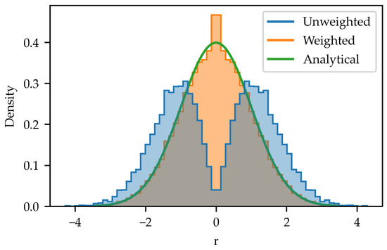
Figure 1.
Densities of samples drawn from the 2D normal distribution with unit variance; (green) analytical radial part of the density function; (blue) density of the radial coordinate of samples; (orange) estimate of radial density using a weighted histogram.
The same artifacts occur when one tries to estimate the density of samples in the transverse phase space (x, y, , ). Here, we take an example distribution in the 4D transverse phase space as being normally distributed with a diagonal covariance matrix. The standard deviation of the spatial coordinates is 1.0, and for the velocities, it is 0.2. We then take samples from this distribution and shear the radial velocities according to for some numbers a and b (here, and ) to arrive at an interesting shape for us to estimate. For the density calculation, the samples are transformed according to the inverse of Equations (2) and (3), and we evaluate a 2D histogram of the coordinates r and weighted by . We show this estimate in Figure 2 (labeled “Histogram”), and one can see the same type of artifacts near that pollute our result.

Figure 2.
Density of points sampled from a beam with nonlinear correlation estimated with the weighted histogram method and the axisymmetric kernel density estimator. The analytical density is shown to the right.
3. The Radial Density
Our goal is to solve the problem of artifacts near when estimating the density of axisymmetric beams. Let us start again with the simpler case of only the spatial coordinates (x and y). To avoid the singular weights of points near the origin, we can start by estimating the density of points in 2D space using the typical Gaussian kernel,
The resulting density estimate (i.e., using Equation (1), it may be evaluated in polar coordinates as . Note that we are not scaling the density by the determinant of the transformation’s Jacobian () because we wish to simply find the original density evaluated at a polar coordinate and not the density of the radial coordinates, which would go to zero like near the origin. This new function, contains an estimate of the radial part at every value of but does not benefit from the known symmetry of the points. To incorporate this, we average over the angular coordinate to obtain .
The density estimator in Cartesian coordinates transformed to polar coordinates and then averaged over the angle should give us an estimate of the density without using the problematic weighting strategy. This integral can be solved analytically, and we find that the kernel is simply replaced by the expression,
where is a modified Bessel function of the first kind. This function is plotted in Figure 3a. If we use the Hankel asymptotic expansion for the Bessel function [18], we find that the behavior as becomes large is
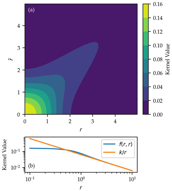
Figure 3.
(a) The averaged kernel for evaluating the axisymmetric radial density of the spatial coordinates; (b) the same function evaluated along compared with its asymptotic form (with ).
This is the typical Gaussian kernel with the expected weighting of along to account for the effect of the growing area element in polar coordinates as r becomes large. We plot this asymptotic expression against the kernel itself along the diagonal in Figure 3b.
Near the origin, however, we see a different behavior. The density no longer has the pole that caused the artifacts we saw in Figure 1. Additionally, back in Figure 3a, if we look along the kernel at fixed , we can see that when the sample is near , there is a boost in the amount of density measured near compared to when the sample is further away. This comes from the averaging over , which means that, for instance, a sample at will also contribute density from the point that can “leak” over the origin and contribute to the estimate when both r and are small. All of these properties, both asymptotic and near the origin, will also show up when we deal with the more complicated case of density estimation for the transverse phase space.
We directly compare density estimates for 10,000 samples drawn from the 2D normal distribution using the weighted histogram described in Section 2 and the axisymmetric kernel density estimator in Figure 4. It is clear that the artifacts near have been reduced to provide a more accurate estimate of the density compared with the analytical value. While experimenting with the density estimator, we found it necessary to use the scaled Bessel function to avoid numerical problems when evaluating the kernel in Equation (5). Fast implementations of the scaled Bessel function are available in many popular scientific computing libraries and have been described in, for example, ref. [19].
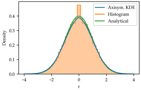
Figure 4.
Comparison between the axisymmetric kernel density estimator (blue), the weighted histogram method (orange), and the analytical expression for the radial part of the 2D density of normally distributed points.
4. Density in Phase Space
With a template of how to proceed from the density estimator of the spatial coordinates, we can begin to derive a kernel for use in phase space. Starting with the Gaussian kernel over the four phase space variables (x, y, , and ), we can transform them according to Equations (2) and (3) and average out over the angular variable, . This gives us the kernel,
with the Bessel function’s argument,
Oftentimes, however, the angular velocity is uninteresting for the beams used in accelerator physics. The samples may have negligible angular velocity, or it may take on a single value for all of the particles such as for magnetized beams. This motivates us to further reduce the number of dimensions by integrating out the dependence of Equation (7) on . We find that the integral can be solved analytically and gives us the kernel,
where the arguments to are
and is the two-argument arctangent that gives the angle from the positive x-axis to the point , and the are,
A detailed derivation of the kernel is given in Appendix A.
The function is an order zero “modified generalized Bessel function” of the first kind with a single parameter (e.g., defined in refs. [20,21]). The function also takes on the integral form,
which can be found by applying the relationship between the modified and unmodified generalized Bessel functions (i.e., Equation (2.22) in ref. [22]) to the typical integral representation (i.e., Equation (2.9) in the same reference). We found that numerically evaluating the logarithm of this integral provides a stable method of calculating its value for use in the kernel. This function’s values may also be tabulated before use in density estimation and then looked up with linear interpolation later to achieve acceptable performance when used with many samples. Further work could be put into deriving an efficient numerical expression for the function’s value using a method similar to how the regular modified Bessel function is computed to improve the speed of evaluating the kernel.
Some examples of the kernel (Equation (9)) for different values of the sample’s location are shown in Figure 5. When the samples have large radius, the function is visually similar to the Gaussian kernel and also falls off with a weighting as was previously found for the case of the spatial coordinates. As the samples move closer to the origin, we also find additional density showing up near . However, unlike in the case of the spatial coordinates, a 180-degree rotation of the sample will take the coordinates to , and so we see the density “leaking over” from a point at and not just the point reflected across . The effect of angular velocity is shown in the second row of Figure 5 and tends to distribute density at a much greater than typical spread of radial velocity after the integration.
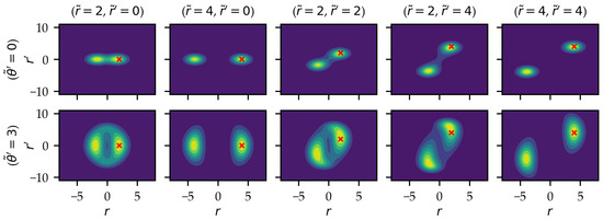
Figure 5.
The averaged phase space kernel (Equation (9)) evaluated for different locations of the sample. The sample’s location is shown as the red cross in each image, and the coordinates are displayed in the header of each column. The angular velocity of the sample is varied along the rows and shown in each row label. The colormaps are normalized to the maximum of the data in each panel to highlight the shape of the kernels rather than their relative magnitude.
We demonstrate the use of this kernel density estimator on the example described in Section 2 of a beam with some nonlinear correlation to the velocities. A set of 50,000 samples was generated, and the densities are shown in Figure 2 using the weighted histogram method and the axisymmetric density estimator with the kernel in Equation (9). This is compared to the analytical value of the density. Visually, it can be seen that the axisymmetric kernel density estimator successfully avoids the problem of artifacts near and matches closely with the analytical distribution. To quantify the difference in accuracy between the two methods at a variety of sample sizes, we numerically evaluated the mean integrated square error (MISE) of the two estimators using 32 samples each time and evaluating the densities on a 64 × 64 grid of values over the same region shown in Figure 2. The results are shown in Figure 6 and suggest that the axisymmetric kernel density estimator successfully avoids artifacts present in the weighted histogram and converges more quickly to the analytical density. Note that these results strongly depend on the choice of the histogram bin size and KDE bandwidth, and for the brief comparison here, we simply used “Scott’s rule of thumb” [17] in both cases.
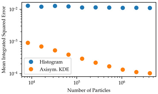
Figure 6.
Estimates of the mean integrated square error of the two density estimators for a variety of sample sizes. For each point, 32 samples were evaluated, and the integrated error was calculated using a 64 × 64 grid of points.
5. Conclusions
In this work, we have derived analytical expressions for two kernel density estimators for use with axisymmetric particle beams: one for the spatial coordinates and one for transverse phase space. These density estimators avoid the problem of artifacts near that result from the need to weight samples in polar coordinates according to the shrinking area element when the radius becomes small. By starting with an estimate of the density in Cartesian coordinates and then averaging over the angle in polar coordinates, we can find estimates of the density that do not diverge as the sample approaches the origin. These estimates should be accurate for any distribution of samples, where the original Cartesian kernel density estimator would give an accurate estimate of density. Being analytical, the expressions avoid the performance and convergence penalties that could come from averaging the kernels numerically. We also note that the longitudinal coordinates can be trivially added to both estimators by multiplying by another Gaussian kernel in those dimensions.
Taking advantage of known symmetries is important to improving the accuracy and performance of numerical algorithms. The density estimators presented here are a stable and efficient method of calculating densities for axisymmetric beams and could help accelerator codes take advantage of the symmetries present in, for example, many photoinjectors. By advancing the ways we design and operate these machines, improved numerical tools will help enable the next generation of particle accelerators.
Author Contributions
Conceptualization, C.M.P.; methodology, C.M.P.; software, C.M.P.; writing—original draft preparation, C.M.P.; writing—review and editing, Y.-K.K.; visualization, C.M.P.; supervision, Y.-K.K.; project administration, Y.-K.K.; funding acquisition, Y.-K.K. All authors have read and agreed to the published version of the manuscript.
Funding
This work was supported by the U.S. National Science Foundation under Award PHY-1549132, the Center for Bright Beams.
Data Availability Statement
No new data were created or analyzed in this study. Data sharing is not applicable to this article.
Conflicts of Interest
The authors declare no conflict of interest.
Appendix A. Calculation of the Phase Space Kernel
To calculate the kernel in Equation (9), we first begin with the Gaussian kernel over the four phase space variables (x, y, , ). The coordinates of both the sample and the point being evaluated are then transformed into polar coordinates according to to Equations (2) and (3) to achieve the expression,
The angular velocity coordinate of the point the kernel is being evaluated at can then be integrated out of this expression with standard techniques to obtain,
We can safely set , as we can see by inspection that our final averaging over angle will no longer depend on the angular coordinate of the data.
The last step in finding the axisymmetric kernel is to perform the averaging of Equation (A2) over the angle of the evaluated point (). This is the integral,
Fortunately, by factoring out terms that do not depend on and rewriting the exponent in Equation (A2) using trigonometric identities, the expression can be made to exactly correspond with the integral form of the modified generalized Bessel function (Equation (12)). This gives us the final form of the axisymmetric kernel shown in Equation (9).
References
- Hockney, R.W.; Eastwood, J.W. Computer Simulation Using Particles; CRC Press: Boca Raton, FL, USA, 2021. [Google Scholar]
- Reiche, S. GENESIS 1.3: A Fully 3D Time-Dependent FEL Simulation Code. Nucl. Instrum. Methods Phys. Res. Sect. Accel. Spectrometers Detect. Assoc. Equip. 1999, 429, 243–248. [Google Scholar] [CrossRef]
- Tran, T.M.; Wurtele, J.S. TDA—A Three-Dimensional Axisymmetric Code for Free-Electron-Laser (FEL) Simulation. Comput. Phys. Commun. 1989, 54, 263–272. [Google Scholar] [CrossRef]
- Edelen, A.L.; Biedron, S.G.; Milton, S.V.; Edelen, J.P. First Steps toward Incorporating Image Based Diagnostics into Particle Accelerator Control Systems Using Convolutional Neural Networks. arXiv 2016, arXiv:physics/1612.05662. [Google Scholar] [CrossRef]
- Lagaris, I.E.; Likas, A.; Fotiadis, D.I. Artificial Neural Networks for Solving Ordinary and Partial Differential Equations. Comput. Phys. 1997, 9, 987–1000. [Google Scholar] [CrossRef]
- Raissi, M.; Perdikaris, P.; Karniadakis, G. Physics-Informed Neural Networks: A Deep Learning Framework for Solving Forward and Inverse Problems Involving Nonlinear Partial Differential Equations. J. Comput. Phys. 2019, 378, 686–707. [Google Scholar] [CrossRef]
- Cuomo, S.; Di Cola, V.S.; Giampaolo, F.; Rozza, G.; Raissi, M.; Piccialli, F. Scientific Machine Learning Through Physics-Informed Neural Networks: Where We Are and What’s Next. J. Sci. Comput. 2022, 92, 88. [Google Scholar] [CrossRef]
- Reiser, M. Theory and Design of Charged Particle Beams, 2nd ed.; Updated and Expanded; Wiley-VCH: Weinheim, Germany, 2008. [Google Scholar]
- Roussel, R.; Edelen, A.; Mayes, C.; Ratner, D.; Gonzalez-Aguilera, J.P.; Kim, S.; Wisniewski, E.; Power, J. Phase Space Reconstruction from Accelerator Beam Measurements Using Neural Networks and Differentiable Simulations. Phys. Rev. Lett. 2023, 130, 145001. [Google Scholar] [CrossRef]
- Mohayai, T.A.; Snopok, P.; Neuffer, D. A Non-Parametric Density Estimation Approach to Measuring Beam Cooling in MICE. arXiv 2018, arXiv:physics/1806.01834. [Google Scholar] [CrossRef]
- Xu, T.; Jing, C.; Kanareykin, A.; Piot, P.; Power, J. Spatio-Temporal Shaping of the Photocathode Laser Pulse for Low-Emittance Shaped Electron Bunches. In Proceedings of the 10th International Particle Accelerator Conference IPAC2019, Melbourne, Australia, 19–24 May 2019; pp. 2163–2166. [Google Scholar] [CrossRef]
- Chen, X.; Yang, L.; Duan, J.; Karniadakis, G.E. Solving Inverse Stochastic Problems from Discrete Particle Observations Using the Fokker–Planck Equation and Physics-Informed Neural Networks. Siam J. Sci. Comput. 2021, 43, B811–B830. [Google Scholar] [CrossRef]
- O’Leary, J.; Paulson, J.A.; Mesbah, A. Stochastic Physics-Informed Neural Ordinary Differential Equations. J. Comput. Phys. 2022, 468, 111466. [Google Scholar] [CrossRef]
- Parzen, E. On Estimation of a Probability Density Function and Mode. Ann. Math. Stat. 1962, 33, 1065–1076. [Google Scholar] [CrossRef]
- Park, B.U.; Marron, J.S. Comparison of Data-Driven Bandwidth Selectors. J. Am. Stat. Assoc. 1990, 85, 66–72. [Google Scholar] [CrossRef]
- Sheather, S.J.; Jones, M.C. A Reliable Data-Based Bandwidth Selection Method for Kernel Density Estimation. J. R. Stat. Soc. Ser. (Methodol.) 1991, 53, 683–690. [Google Scholar] [CrossRef]
- Jones, M.C.; Marron, J.S.; Sheather, S.J. A Brief Survey of Bandwidth Selection for Density Estimation. J. Am. Stat. Assoc. 1996, 91, 401–407. [Google Scholar] [CrossRef]
- Abramowitz, M.; Stegun, I.A. Handbook of Mathematical Functions: With Formulas, Graphs and Mathematical Tables. Dover Books on Advanced Mathematics; Dover Publications: Mineola, NY, USA, 1972. [Google Scholar]
- Press, W.H.; Vetterling, W.T.; Teukolsky, S.A.; Flannery, B.P. Numerical Recipes in C++: The Art of Scientific Computing, 2nd ed.; Cambridge University Press: New York, NY, USA, 2001. [Google Scholar]
- Dattoli, G.; Giannessi, L.; Mezi, L.; Torre, A. Theory of Generalized Bessel Functions. Nuovo C. Ser. 1990, 105, 327–348. [Google Scholar] [CrossRef]
- Dattoli, G.; Torre, A.; Lorenzutta, S.; Maino, G.; Chiccoli, C. Theory of Generalized Bessel Functions.-II. Nuovo C. B 1991, 106, 21–51. [Google Scholar] [CrossRef]
- Dattoli, G.; Chiccoli, C.; Lorenzutta, S.; Maino, G.; Richetta, M.; Torre, A. Advances on the Theory of Generalized Bessel Functions and Applications to Multiphoton Processes. J. Sci. Comput. 1993, 8, 69–109. [Google Scholar] [CrossRef]
Disclaimer/Publisher’s Note: The statements, opinions and data contained in all publications are solely those of the individual author(s) and contributor(s) and not of MDPI and/or the editor(s). MDPI and/or the editor(s) disclaim responsibility for any injury to people or property resulting from any ideas, methods, instructions or products referred to in the content. |
© 2023 by the authors. Licensee MDPI, Basel, Switzerland. This article is an open access article distributed under the terms and conditions of the Creative Commons Attribution (CC BY) license (https://creativecommons.org/licenses/by/4.0/).