

FASER’s Electromagnetic Calorimeter Test Beam Studies

Abstract
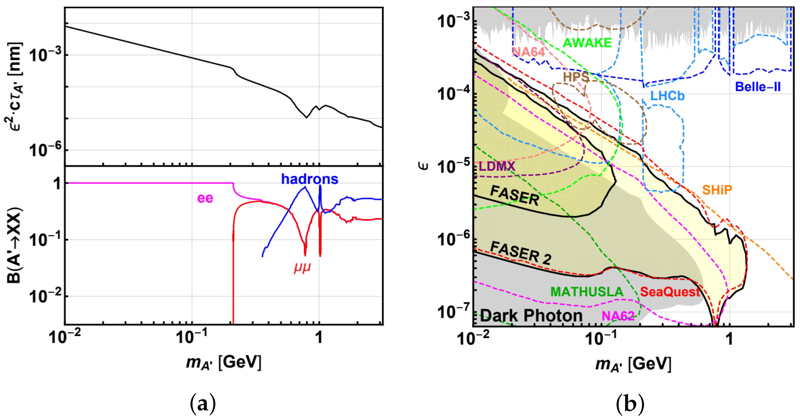
:1. Introduction
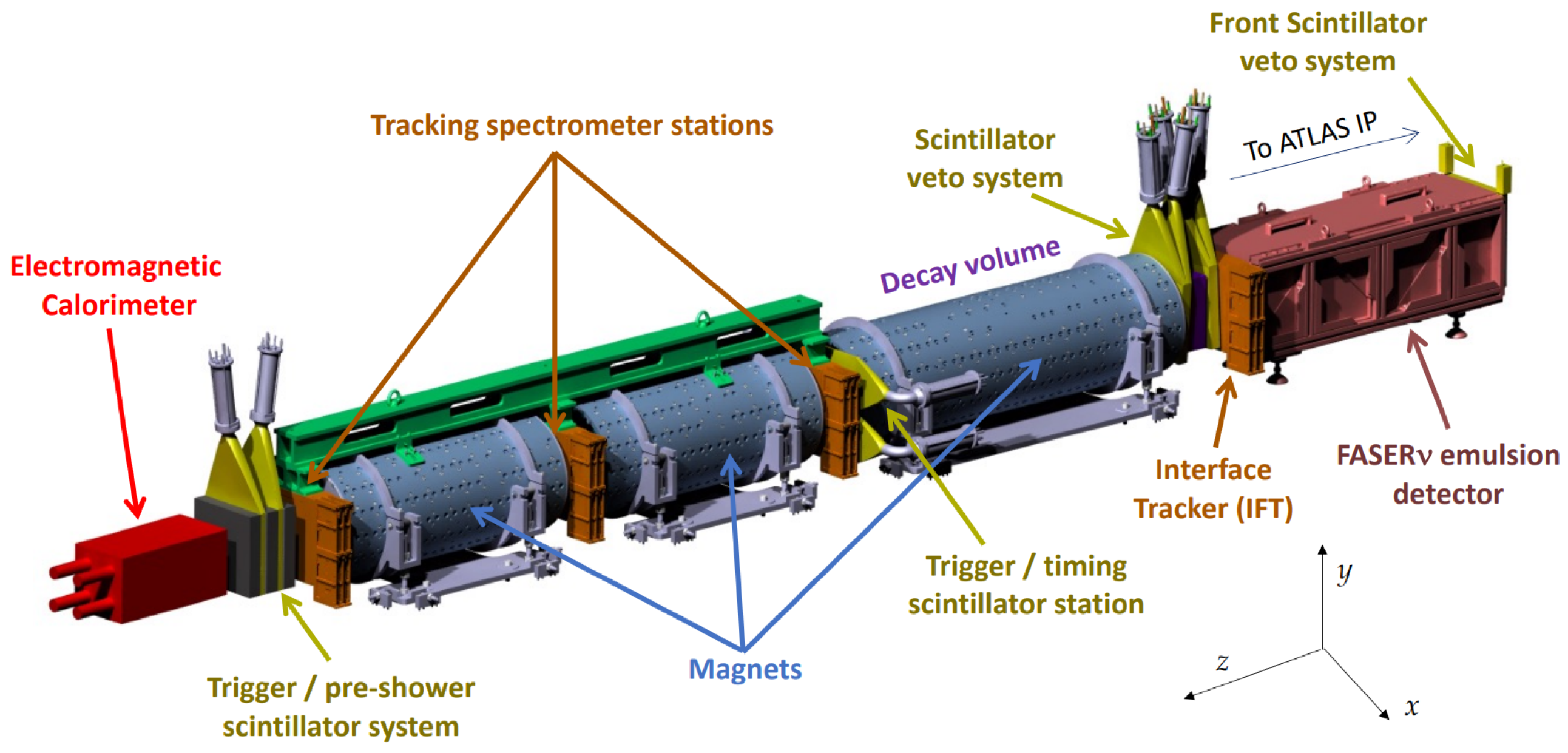
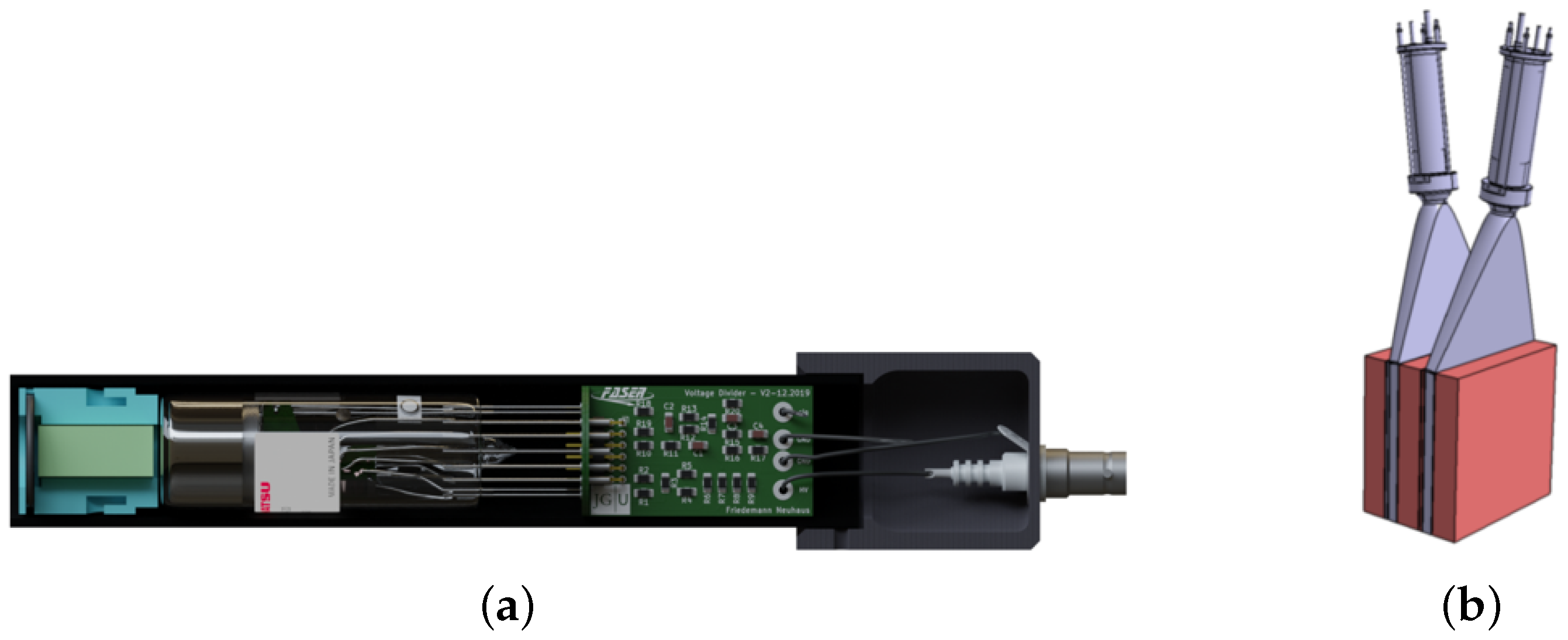
2. The FASER Experiment
3. Results of the 2021 FASER Calorimeter Test Beam
3.1. Aims and Overview
3.2. Data Analysis
- The event trigger bit must indicate that the front two trigger scintillators were hit.
- Only one track must be found in the event, with tracks reconstructed according to a dedicated tracking algorithm.
- Tracks must be relatively straight with angle cuts such that the angular spread in the x and y plane is and degrees.
- The track position must be within a 20 mm × 20 mm square area surrounding the beam position, obtained from extrapolating the track to the face of the calorimeter.
3.3. Test Beam Simulation
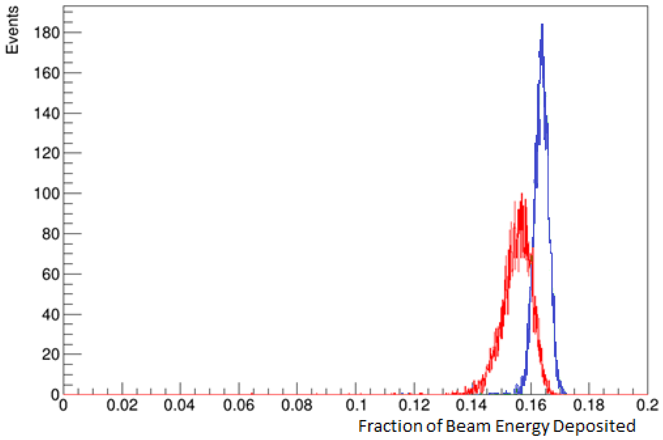
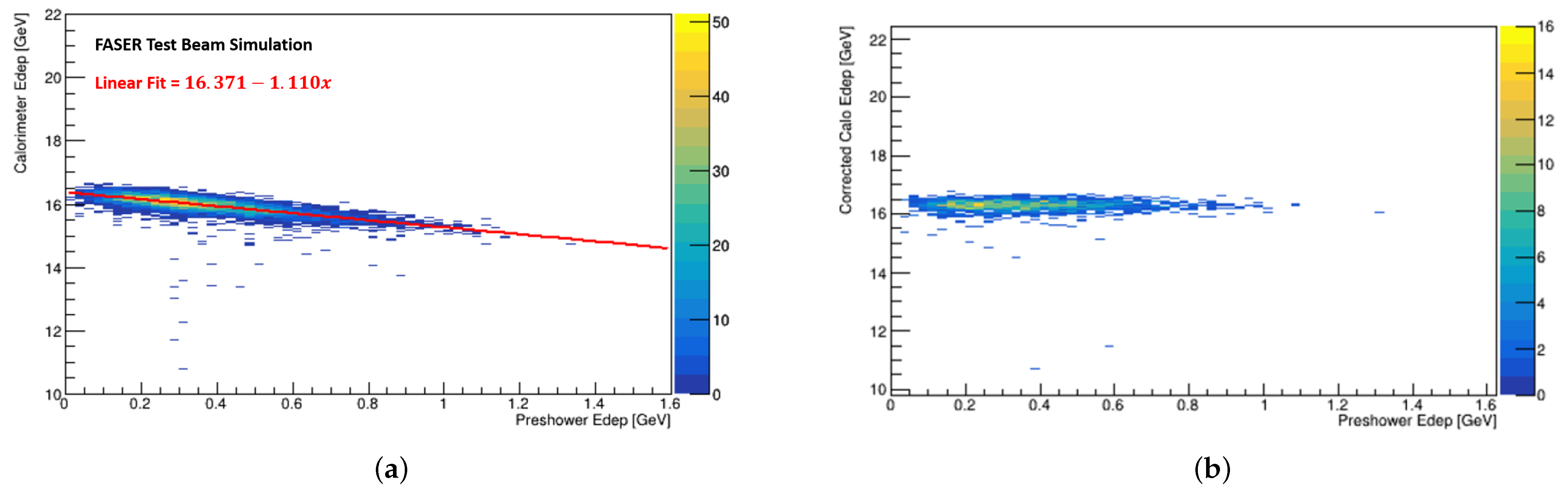
3.4. Pre-Shower Correction
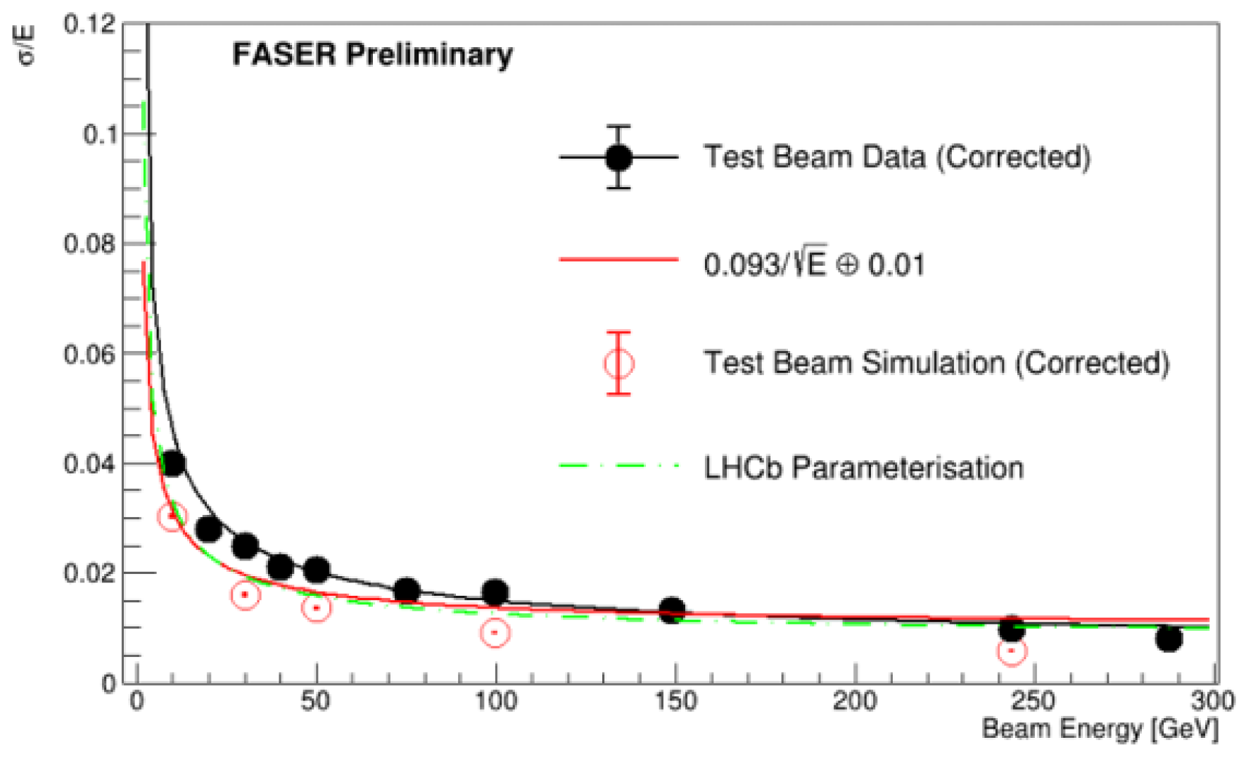
3.5. Energy Resolution
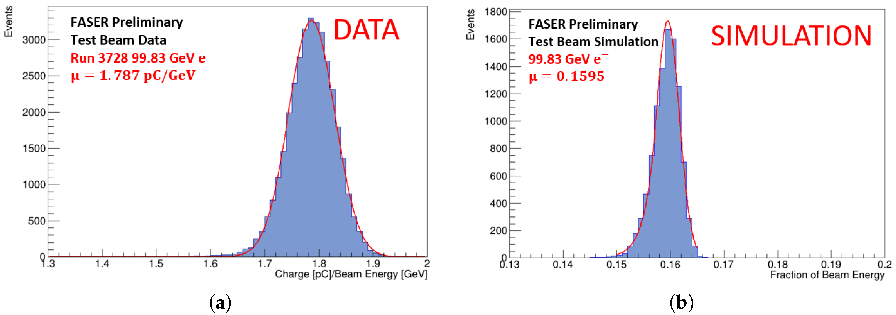
3.6. Energy Calibration
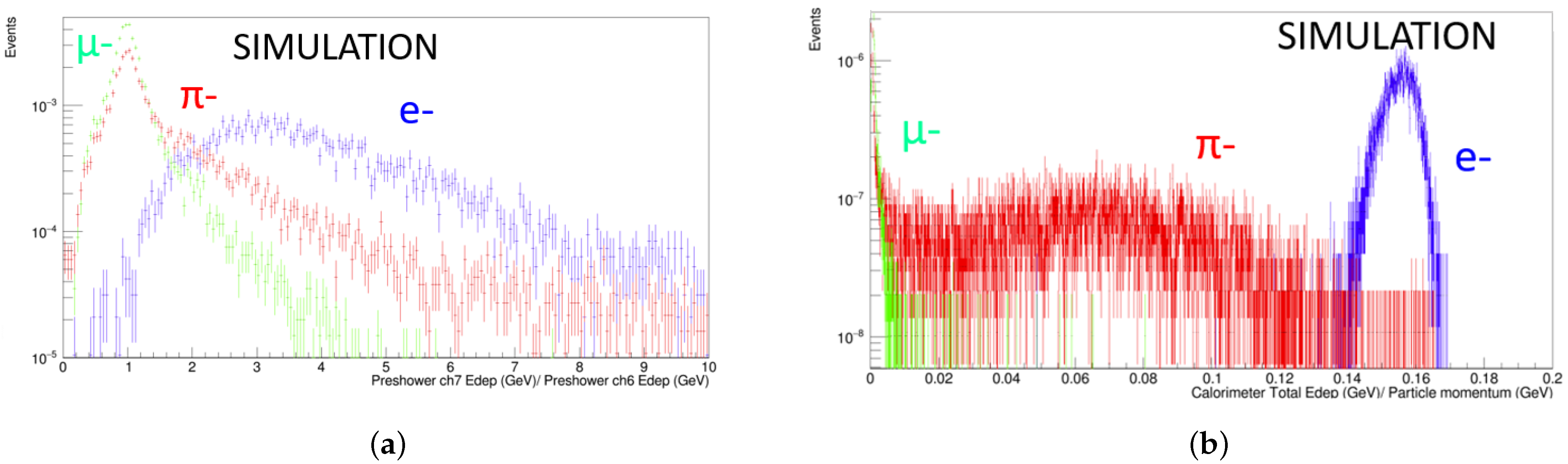
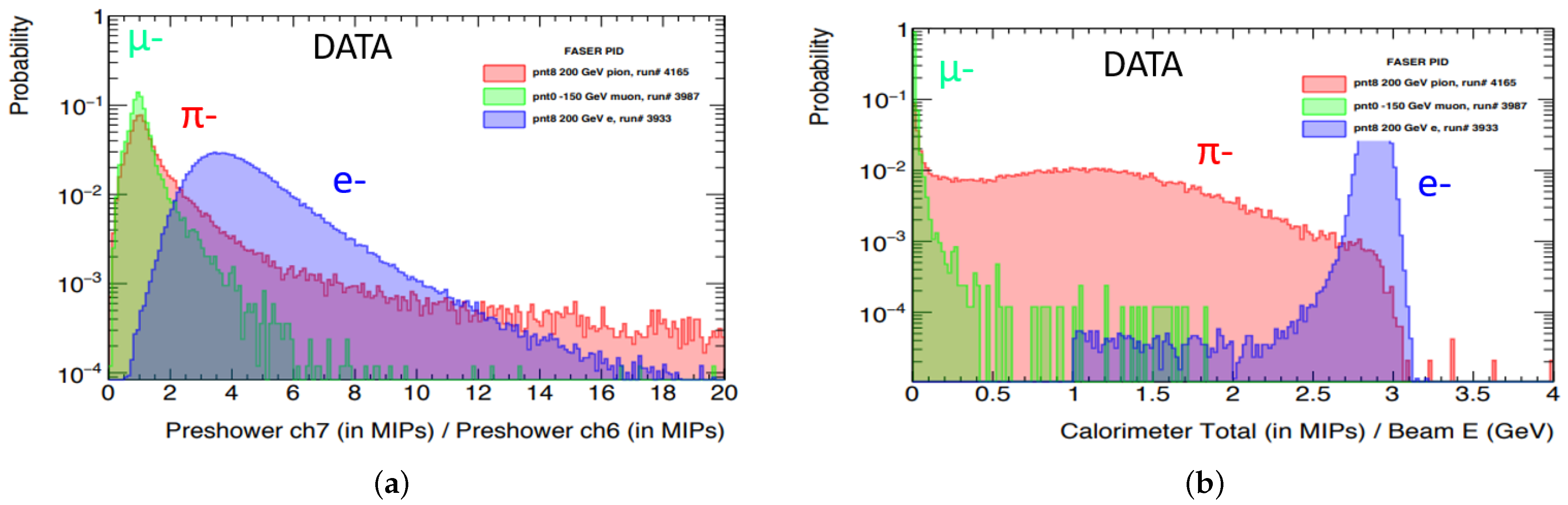
3.7. PID Capabilities
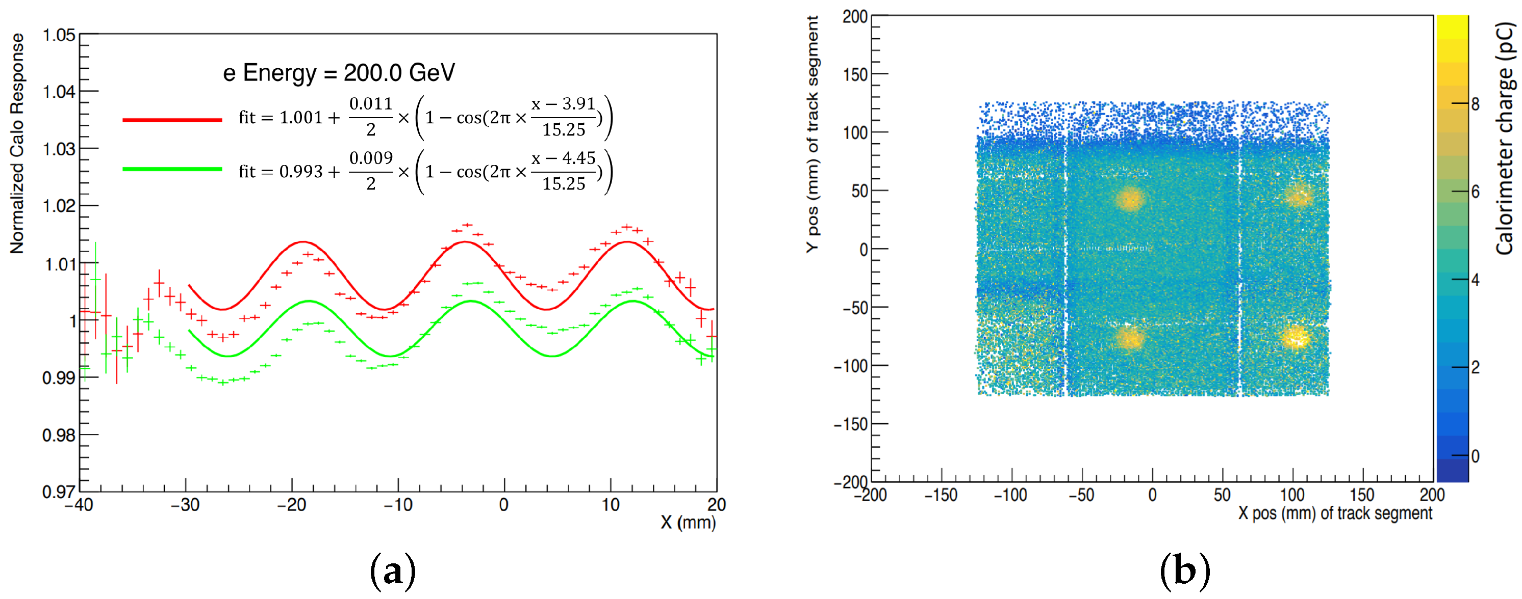
3.8. Local Calorimeter Effects
4. Conclusions
Funding
Data Availability Statement
Acknowledgments
Conflicts of Interest
Abbreviations
| FASER | Forward Search Experiment at the LHC | IFT | Interface Tracker |
| ALP | Axion-like Particle | ECAL | Electromagetic Calorimeter |
| LLP | Long-lived Particle | xAOD | Analysis Object Data |
| SM | Standard Model | ADC | Analogue to Digital Conversion |
| DS | Dark Sector | WLS | Wavelength Shifting Fibre |
| IP1 | ATLAS Interaction Point | MIP | Minimum Ionising Particle |
| SCT | ATLAS Semiconductor Tracker | PMT | Photomultiplier Tube |
| PID | Particle Identification |
References
- Ariga, A.; Abreu, H.; Mansour, E.A.; Antel, C.; Ariga, T.; Bernlochner, F.; Boeckh, T.; Boyd, J.; Brenner, L.; Cadoux, F.; et al. The FASER Detector. CERN-FASER-2022-001. arXiv 2022, arXiv:2207.11427. [Google Scholar]
- Ariga, A.; Ariga, T.; Boyd, J.; Cadoux, F.; Casper, D.W.; Favre, Y.; Feng, J.L.; Ferrere, D.; Galon, I.; Gonzalez-Sevilla, S.; et al. Technical Proposal: FASER, the Forward Search Experiment at the LHC; Tech. Rep. CERN-LHCC-2018-036. LHCC-P-013; CERN: Geneva, Switzerland, December 2018; Available online: http://cds.cern.ch/record/2651328 (accessed on 24 July 2022).
- Ariga, A.; Ariga, T.; Boyd, J.; Cadoux, F.; Casper, D.W.; Favre, Y.; Feng, J.L.; Ferrere, D.; Galon, I.; Gonzalez-Sevilla, S.; et al. FASER’s Physics Reach for Long-lived Particles. Phys. Rev. D 2019, 99, 095011. [Google Scholar] [CrossRef]
- Battaglieri, M.; Belloni, A.; Chou, A.; Cushman, P.; Echenard, B.; Essig, R.; Estrada, J.; Feng, J.L.; Flaugher, B.; Fox, P.J.; et al. US Cosmic Visions: New Ideas in Dark Matter 2017: Community Report. arXiv 2017, arXiv:1707.04591. [Google Scholar]
- Abdesselam, A.; Akimoto, T.; Allport, P.P.; Alonso, J.; Anderson, B.; Andricek, L.; Anghinolfi, F.; Apsimon, R.J.; Barbier, G.; MacWaters, C.; et al. The barrel modules of the ATLAS semiconductor tracker. Nucl. Instrum. Meth. A 2006, 568, 642–671. [Google Scholar] [CrossRef] [Green Version]
- LHCb Collaboration. LHCb Calorimeters: Technical Design Report; CERN: Geneva, Switzerland, 2000; Available online: http://cds.cern.ch/record/494264 (accessed on 24 July 2022).
- H2 Beam Line. Available online: http://sba.web.cern.ch/sba/BeamsAndAreas/H2/H2_presentation.html (accessed on 24 July 2022).
- Geant4 Collaboration. CERN. Available online: https://geant4.web.cern.ch/ (accessed on 24 July 2022).
- ATLAS Collaboration. The VP1 ATLAS 3D Event Display. Available online: http://atlas-vp1.web.cern.ch/ (accessed on 24 July 2022).
- Arefev, A.; Kvaratskheliia, T.; Morozov, A.; Melnikov, E.; Voronchev, K.; Roussinov, D.; Barsuk, S.; Belyaev, I.; Bobchencko, B.; Martemyanov, M.; et al. Beam Test Results of the LHCb Electromagnetic Calorimeter; CERN-LHCB-2007-149; CERN: Geneva, Switzerland, 2008. [Google Scholar]


| Energy | With Pre-Shower | Tungsten/Graphite Removed |
|---|---|---|
| 30 GeV | 2.72 ± 0.04% | 1.58 ± 0.02% |
| 200 GeV | 0.9 ± 0.01% | 0.71 ± 0.01% |
| Energy | With Pre-Shower | Tungsten/Graphite Removed |
|---|---|---|
| 30 GeV | 3.76 ± 0.03% | 2.84 ± 0.02% |
| 200 GeV | 1.89 ± 0.01% | 1.67 ± 0.01% |
| a | b | c | |
| Data (Corrected) | 0.134 | 0.151 | 0.0065 |
| Data | 0.196 | 0.151 | 0.0057 |
| Simulation (Corrected) | 0.093 ± 0.003 | - | 0.0000 ± 0.0004 |
| Simulation | 0.135 ± 0.001 | - | 0.0000 ± 0.0017 |
| LHCb | 0.094 ± 0.004 | 0.108 ± 0.029 | 0.0083 ± 0.0002 |
Publisher’s Note: MDPI stays neutral with regard to jurisdictional claims in published maps and institutional affiliations. |
© 2022 by the author. Licensee MDPI, Basel, Switzerland. This article is an open access article distributed under the terms and conditions of the Creative Commons Attribution (CC BY) license (https://creativecommons.org/licenses/by/4.0/).
Share and Cite
Cavanagh, C., on behalf of the FASER Collaboration. FASER’s Electromagnetic Calorimeter Test Beam Studies. Instruments 2022, 6, 31. https://doi.org/10.3390/instruments6030031
Cavanagh C on behalf of the FASER Collaboration. FASER’s Electromagnetic Calorimeter Test Beam Studies. Instruments. 2022; 6(3):31. https://doi.org/10.3390/instruments6030031
Chicago/Turabian StyleCavanagh, Charlotte on behalf of the FASER Collaboration. 2022. "FASER’s Electromagnetic Calorimeter Test Beam Studies" Instruments 6, no. 3: 31. https://doi.org/10.3390/instruments6030031
APA StyleCavanagh, C., on behalf of the FASER Collaboration. (2022). FASER’s Electromagnetic Calorimeter Test Beam Studies. Instruments, 6(3), 31. https://doi.org/10.3390/instruments6030031