Abstract
We describe the design and construction of coils to compensate the Earth’s magnetic field in the vertical cryostat GERSEMI in the FREIA laboratory at Uppsala University.
1. Introduction
We discuss the design and installation of coils to compensate the Earth’s magnetic or any other stray fields in the vertical cryostat, named GERSEMI (GERSEMI is the daughter of FREIA according to Nordic mythology.) In the FREIA laboratory. The cryostat was originally designed for magnet tests and lacks magnetic shielding. In order to maintain the option to use it for testing superconducting radio-frequency cavities a magnetic shield or compensation of external fields was deemed necessary. Given all constraints, we targeted an accuracy on the order of T, or a few percent of the Earth’s magnetic field magnitude.
In this report, we discuss the system that we retro-fitted to the cryostat. Since the cryostat was already under construction, we were constrained to mount the compensation coils to the walls of the vertical hole for the cryostat, which has a diameter of 2 m and is close to 5 m deep. An RF-cavity will likely be placed near the bottom, say the lower 2 or 3 m of the hole. For a first estimate of the required currents for the coils we assume perfect Helmholtz coil geometry, where the distance between coils equals their radius. Here the radius is m. In that case the magnetic field in the center of the coils, separated by a distance R is given by such that A-turns will provide a field of about T. Thus a coil with turns and a power supply for 10 A or more would be suitable. We estimate the voltage and power to drive 10 A through 10 turns of radius m we assume to use a copper wire with a diameter of 1.5 mm. The resistivity of copper is m and the resistance of the wire with 10 turns is which results in a voltage of V and a power dissipation of W.
After these first estimates, we turn to calculating the field in the vertical hole due to a more realistic geometry of the coils.
2. Coil Geometry
With the given radius m the axial extent of the good field region is only ±0.2 m, such that we decided to increase it using three axial coils for the vertical field component . Experimenting with multiple coils [1] we found that placing the three coils with a winding ratio and spaced by 1 m results in a reasonably good-field region of ±0.8 m in which the relative field variation is 1.2% peak-to-peak. Figure 1 shows the resulting vertical field component as a function of This was deemed acceptable.
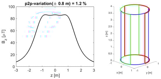
Figure 1.
(Left): Axial field as a function of z. (Right): geometry of the three radial coils, shown in red, green, and blue, respectively, each with two vertical wires connected by semi-circular arcs on both ends.
In order to compensate previously unknown stray fields, we wanted to control the radial field components and to point in any direction. Therefore, inspired by the way of how three-phase AC-motors operate, we investigated a configuration with three coils placed with 120 degrees in between to control the magnetic field vector in the -plane. The wiring of the coils is shown on the right-hand side in Figure 1 as the dashed lines. The three coils are excited by three power supplies, excited with 120 degree phase separation between adjacent coils, in the following pattern
where is the maximum current that determines the magnitude of the excitation and the direction. In simple two-dimensional simulations, we found the radial field component within a circle of m radius to vary by about 3% peak-to-peak.
3. The Real Geometry
A sketch of the geometry, adapted to the available space in GERSEMI, is shown on the left-hand side in Figure 2 with the axial coils shown in magenta and the three axial coils red, green, and blue. The three-phase radial -coils extend vertically from to m and the three axial -coils are placed at and m. The photograph on the right-hand side in Figure 2 shows the coils after they were mounted in the vertical hole for the cryostat with the cables enclosed in piping, normally used for sanitary installations. The three circular pipes at height 0.9, 1.9, ad 2.9 m from the bottom contain the windings for the coils that create the vertical field component. The circular pipes at the bottom and the top are the return path for the coils that create the radial field components for which the wires are color-coded in red, blue and brown. The coil with the brown cables starts at the left-hand side of the image and extends along the top to the right-hand side. Note that this correction of an externally generated field is conceptually different from shimming iron-dominated magnets by additional pieces of iron or coils.
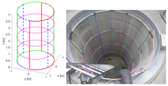
Figure 2.
(Left): the geometry with the three axial coils in magenta and the three axial coils colored red, green, and blue. (Right): photograph of the coils (with superimposed colors), enclosed in plastic pipes and installed in the hole for the cryostat. The axial coil arcs, connecting the vertically mounted radial coils, are visible near the top and the bottom of the hole.
We simulate this geometry with a simple magnetic field solver [1] based on solving Biot–Savart’s equation for a straight, current-carrying line segment and approximating the geometry of lines and arcs by polygons consisting of short segments. Summing the contributions from all segments gives the field at an arbitrary point. This method is suitable for calculating fields in the absence of magnetic materials.
Figure 3 shows the axial (left) and radial (right) field component along the vertical axis of the hole. We see that shows the three humps due to the three-coil configuration. The field is within 10% of the center value between and 3.1 m. The radial component, shown on the bottom rolls off below 1 and above 3 m. Here the 10% margin is reached approximately at and 3.1 m. The roll-off of the radial field is accompanied by an increase of the axial field, which increases the “unwanted” field component below 1 and above 3 m. We cannot do anything about this roll-off, except making the radius of the coils bigger or adding additional coils. Deciding how much to lower the cavity into the “bad field” region is a matter of the gradient and the dependence of the quench limits on the magnetic field.
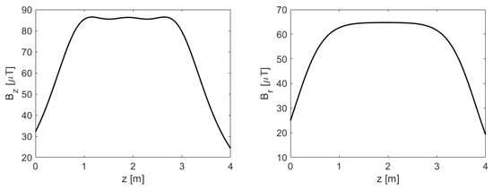
Figure 3.
The axial (left) and radial (right) component of the magnetic field on the axis. The current is assumed to be 10 A.
4. Compensating the Residual Field
After installing the coils we used the PhyPhox software [2] on a smartphone to measure the magnetic field at the expected position for the cavities. We then excited each of the coils, one at a time, with 10 A and recorded the fields. The results collected in the following Table 1:

Table 1.
Magnetic fields caused by passing 10 A through the coils, one at a time.
The first column, labeled “All Off” shows the residual field without compensation and the subsequent columns the measured field with the 10 A excitation of the coils.
It is obvious that the solenoidal coils predominantly affect the vertical field component and we see that the response of on the Solenoid current is given by
Furthermore, we have three coils to minimize the two horizontal field components and This under-determined system can, however, be solved with the help of Singular Value Decomposition (SVD), which is the method of choice to treat such problems [3]. To do so, we first build the response matrix A of the horizontal magnetic field components on the coil excitations and then use SVD to write
where U and W are orthogonal matrices and V is diagonal. The degeneracy causes one of its eigenvalues to be zero. We invert the system projecting out the degenerate subspace by setting the inverse of the zero eigenvalue also to zero [3], and re-assembling the inverse of A. Applying to the measured field components then yields the required excitation currents for the coils to compensate for the field. The following code, using MATLAB notation, implements this method.
    % calibration.m
    L0=[-2;27]; L1=[-3;-19]; L2=[-42;45]; L3=[40;42];
    A=[L1-L0,L2-L0,L3-L0]/10;
    [U,V,W]=svd(A)
    iV=diag([1/V(1,1),1/V(2,2),0])
    Corr=-W*iV(:,1:2)*U’
    Bmeas=[-2;27];
    currents=Corr*Bmeas
    result=Bmeas+A*currents
    dIsol_over_dBz = -10/(-190+78).
At the top of the script, the measurements for and are entered and used to build the matrix A that is subsequently decomposed into the three matrices and W. The inverted matrix with the smallest zero-eigenvalue replaced by zero is the correction matrix. The corresponding equations are then
such that entering the measured fields at zero current (the first column in the table) yields the currents with which to excite the coils. They are given by
Dialing in these currents to the power supplies resulted in fields at the level of T such that no further corrections were needed. The fields at locations away from the point where we measured the fields are determined by the geometry of the coils and can be readily calculated with simulation codes, but not independently adjusted by our system.
We point out that with the presented algorithm the magnetic field vector can be set to any value within the limits of the power supplies. This will enable us to even compensate small changes in the background magnetization, should they arise after magnet tests. Moreover, we can perform limited de-Gaussing by cycling the current in the coils with decreasing magnitude, in order to remove this magnetization.
5. Control
We employed DELTA 7020D power supplies [4], inherited from another experiment. Unfortunately, they were not equipped with a control system interface. On the other hand, they all have an analog control interface that provides a reference voltage and control inputs to adjust voltage or current. Moreover, read-back values for voltage and current, as well as supervisory parameters are available. We, therefore, built a small circuit board for a MCP4922 [5] 12-bit dual digital-to-analog converter (DAC) with an SPI interface and plug it on top of an Arduino UNO [6] that is equipped with an Ethernet shield [7]. We use the reference voltage, provided from the power supply as reference for the DAC and program on the UNO listens to either the serial line (via USB) or on an Ethernet port to receive text strings that follow a simplified command set, inspired by the Standard Commands for Programmable Instrumentation (SCPI) [8]. For example, the command DACA nnn sets one of the converters to value nnn. Calibrated input from physical values (Ampere) is also available. All read-back values are monitored and can be queried. For example, sending IOUTA? to query the output current of channel A returns IOUTA val. The implementation is based on code examples from [9].
Interfacing an SCPI-based device to our EPICS [10] control system is straightforward. We only have to prepare protocol files to describe the low-level communication, such as
  set_DACA{out "DACA %u"; ExtraInput = Ignore;}
  get_current{out "IOUTA?"; in "IOUTA %f"; ExtraInput = Ignore;}
and using it as a stream device [11]. Again, the implementation closely follows [9].6. Conclusions
After designing and building the coils we verified that they can be flexibly used to adjust the magnetic field inside the vertical hole for the GERSEMI cryostat to zero or to any other value and direction within the limits of the power supplies. We also built the power supply controller for two channels that is bench tested and will be deployed shortly, but in time before the first magnets and cavities arrive later this spring.
Author Contributions
Conceptualization, V.Z.; data curation, R.W. and A.W.; methodology, T.P.; resources, A.W.; writing—original draft, V.Z. All authors have read and agreed to the published version of the manuscript.
Funding
This research received no external funding.
Acknowledgments
We acknowledge fruitful discussions with Lars Hermansson, Konrad Gajewski, Rocio Santiago-Kern, and Roger Ruber.
Conflicts of Interest
The authors declare no conflict of interest.
References
- Ziemann, V.; Wedberg, R.; Peterson, T.; Wiren, A. Earth-field Compensation Coils for the Vertical Cryostat in FREIA; FREIA-Report 2018-01; Uppsala University: Uppsala, Sweden, January 2018. [Google Scholar]
- PhyPhox. Physical Phone Experiments. Available online: http://phyphox.org (accessed on 7 March 2020).
- Press, W.H.; Flannery, B.P.; Teukolsky, S.A.; Vetterling, W.T. Numerical Recipes, 2nd ed.; Cambridge University Press: Cambridge, UK, 1992. [Google Scholar]
- Delta Elektronika. Overview of Discontinued DC Power Supplies. Available online: https://www.delta-elektronika.nl/en/support/discontinued-products.html (accessed on 7 March 2020).
- Microchip Technology Inc. MCP4922. Available online: https://www.microchip.com/wwwproducts/en/MCP4922 (accessed on 7 March 2020).
- Arduino. Available online: https://www.arduino.cc (accessed on 7 March 2020).
- Arduino. Arduino Ethernet Shield V1. Available online: https://www.arduino.cc/en/Main/ArduinoEthernetShieldV1 (accessed on 7 March 2020).
- IVI Foundation. Available online: https://www.ivifoundation.org/scpi/default.aspx (accessed on 7 March 2020).
- Ziemann, V. A Hands-on Course in Sensors using the Arduino and Raspberry Pi; CRC Press: Baton Rouge, LA, USA, 2018. [Google Scholar]
- Experimental Physics and Industrial Control System. Available online: https://epics.anl.gov/ (accessed on 7 March 2020).
- EPICS at PSI. Available online: http://epics.web.psi.ch/software/streamdevice (accessed on 7 March 2020).
© 2020 by the authors. Licensee MDPI, Basel, Switzerland. This article is an open access article distributed under the terms and conditions of the Creative Commons Attribution (CC BY) license (http://creativecommons.org/licenses/by/4.0/).