The Cramer—Rao Inequality to Improve the Resolution of the Least-Squares Method in Track Fitting

Abstract

The Cramer–Rao–Frechet inequality is reviewed and extended to track fitting. A diffused opinion attributes to this inequality the limitation of the resolution of the track fits with the number N of observations. It will be shown that this opinion is incorrect, the weighted least squares method is not subjected to that N-limitation and the resolution can be improved beyond those limits. In previous publications, simulations with realistic models and simple Gaussian models produced interesting results: linear growths of the peaks of the distributions of the fitted parameters with the number N of observations, much faster than the $\sqrt{\mathrm{N}}$ of the standard least-squares. These results could be considered a violation of a well-known $1/\mathrm{N}$-rule for the variance of an unbiased estimator, frequently reported as the Cramer–Rao–Frechet bound. To clarify this point beyond any doubt, a direct proof of the consistency of those results with this inequality would be essential. Unfortunately, such proof is lacking. Hence, the Cramer–Rao–Frechet developments are applied to prove the efficiency (optimality) of the simple Gaussian model and the consistency of the linear growth. The inequality remains valid even for irregular models supporting the similar improvement of resolution for the realistic models.

1. Introduction

Track reconstruction is a fundamental tool in experimental particle physics, which justifies the large efforts in hardware and software dedicated to its improvements. As part of these efforts, we started to develop new fitting tools based on studies of the signal patterns released by minimum ionizing particles (MIPs) in silicon detectors [1,2]. It is evident that any information acquired by a detector is precious to improve the track reconstruction. To properly handle these pieces of information, we developed a set of mathematical methods to calculate a probability density function (PDF) for each hit. The non-Gaussian forms of the PDFs oblige the use of the maximum likelihood search for the fits. This search on products of PDFs for the hits of each track gives very large improvements in the resolution of all the track parameters and shows insensitivity to outliers. Among the new fitting results, one looks particularly attractive [2], it shows a linear growth of the momentum distributions with the number N of detecting layers. This linear growth is much faster than the growth of the standard least-squares method that cannot increase faster than $\sqrt{\mathrm{N}}$. This effect could not be discussed with the due details in ref. [2], it contained too many different arguments to add other. Therefore, ref. [3] was entirely dedicated to the description of the linear growth. A section of ref. [3] deals with a simplified illustration of the mechanism of its production. For this, we developed a Gaussian toy-model able to an easy reproduction of some our results. The simplicity of the toy-model allows the development of analytical expressions (some pages of mathematics) that completely describe the model. Instead of equations, we prefer to prepare an easy simulation to be contained in a few lines of MATLAB code. The results of this toy-model have a very effective visual impact for the unusual slenderness of the parameter distributions (empirical PDFs) and their fast growth with N. Nothing to do with the slow growth of the corresponding PDFs of the standard fit. Such evident differences could activate reminiscences of mathematical statistics where the $\sqrt{\mathrm{N}}$ is a frequent result. In particular, the widely reported form of the Cramer–Rao–Frechet (CRF) bound was used to raise doubts [4] on the generality of these fast growths. To dissipate forever any possible doubt and to defend our growth (linear or faster than linear) against any criticism, we are forced to recall the necessary details of the CRF method to demonstrate the consistency of our results with the CRF-inequality. To illustrate better what spurred us on this exploration of the CRF technologies, we report some results of the Gaussian toy-model, with a few details of its construction. In principle, there is no need to know these details for the following mathematical developments, they are completely self-contained. Instead, the results of the toy-model are relevant to give a dimension to the practical effects of the versions of the CRF-inequality that will be developed. Those practical effects are invisible in the very simple aspect of the inequalities. At the same time, the mathematical results give an extended generality to the improvements of these fitting methods.

The following Figure 1 illustrates (Monte Carlo) simulations of a simple tracker with N detecting layers of identical technology (silicon microstrips) crossed at orthogonal incidence by a set of parallel straight tracks of minimum ionizing particles (MIPs). The reported estimator is the track direction (the tangent of a small angle). In this toy-model, the hit uncertainties are Gaussian distributions with two type of hit quality. One of very good quality when the MIP crosses the detector near the borders ($20\%$ of strip width), and the other of bad quality ($80\%$ of the strip width) around the strip center. The standard deviations of the hit Gaussian distributions are ${\sigma }_1=0.18$ and ${\sigma }_2=0.018$ strip widths (the strip width is 63 $\mathsf{\mu }$m). (These models with non-identical variances are called heteroscedastic in statistics.) The simulated orthogonal straight tracks (produced and organized as described in Appendix B) are fitted with two different least-squares methods, one that uses only the hit positions and the second that also uses the hit quality (weighted least-squares).

With standard least-squares, we define the usual least-squares where all the inserted observations have identical variances (homoscedastic models). The standard least-squares, built for homoscedastic models, when applied to heteroscedastic models gives results almost insensitive to the presence of the good hits, the maximums of the empirical PDFs show a growth very near $\sqrt{\mathrm{N}}$. The blue lines of Figure 1. Instead, the weighted least-squares, in this heteroscedastic model, has an almost linear growth of the maximums of the empirical PDFs. Translating these results on mean variances, the standard fit shows a $1/\mathrm{N}$ trend, instead, the weighted fit shows a trend of the mean variances as $1/{\mathrm{N}}^2$. It is just this trend $1/{\mathrm{N}}^2$ that could be considered a violation of the CRF-bound as reported in many books and documentations. However, the main part of ref. [3] deals with physical models with Cauchy-like tails and (in theory) with infinite variance. Hence, any finite lower bound on the variance, given by the CRF-inequality, is automatically satisfied by them. In any case, the evident similarity of the PDFs of the physical models with those of the Gaussian toy-model could extend to their linear growth doubts similar to those of the toy-model. Therefore, we must explore the CRF-inequality to prove the inappropriate extension [4] of the rule $1/\mathrm{N}$ outside its domain of validity. For this, we will extend the CRF developments to heteroscedastic models and to the least squares method for track fitting (for straight tracks and curved tracks) with a special attention to our Gaussian model. We did not find the last two points in the literature. The interest in CRF-inequality moves in field very far from track fitting as illustrated by ref. [5] and therein references. Even if the essential equations are very similar, and our tracks are stochastic processes, it is better to develop our approach in direct connection to our problem with a strict reference to the equations used in refs. [1,2,3]. If other authors did similar developments we apologize for not citing them. In any case, the enormous statistical samples of tracks (of the order of ${10}^{12}$ tracks per year) renders very important careful studies of any detail of their fitting methods and the selection of the best. The use of the appropriate fitting tools in heteroscedastic systems allows drastic improvements of the quality of the track reconstruction. The lucky model of ref. [3] is a first order tool to account for the heteroscedasticity of the silicon trackers.

Section 2 recall the essential definitions and the demonstration of the simplest form of the CRF-inequality in the case of the independent and identically distributed (i.i.d.) random variables. Section 3 contains a first model of heteroscedasticity, the weighted mean and its efficiency (optimality) compared to the standard (arithmetic) mean. In Section 4 we apply the CRF-inequality to the least-squares for straight tracks with the corresponding estimator definitions, it is proved that in heteroscedastic system the estimators of standard least-squares have greater variances compared to the heteroscedastic ones. Section 5 deals with the momentum estimators in a simplified model of high-momentum tracks. The conclusions are in Section 6. We added in Appendix A with a few essential properties of the positive semi-definite matrices used in Section 4 and Section 5. Appendix B contains details about the Gaussian toy-model.

2. The Standard CRF-Inequality

The developments of this section follow as far as possible refs. [6,7]. As usual it is considered a N-times repetition of random observations $\{x_1,x_2\dots x_N\}$ described by an identical probability density function (PDF) $f(x,\theta )$, where $\theta$ is a (scalar) parameter. The variables $\mathbf{x}=\{x_1,x_2\dots x_N\}$ are i.i.d. random variables. We will not comment the absolute physical inconsistency of this assumption. The probability of the set $\mathbf{x}$ of i.i.d. random variables (likelihood function) is:

$$L(\mathbf{x},\theta )=f(x_1,\theta )f(x_2,\theta )\dots \dots f(x_N,\theta ) .$$

(1)

As usual $f(x,\theta )$ is positive, normalized, and supposed differentiable with respect to the $\theta$-parameter. Let us define the random variable $U(\mathbf{x},\theta )$:

$$U(\mathbf{x},\theta )=\frac{\partial ln L(\mathbf{x},\theta )}{\partial \theta }=\sum _{i=1}^N\frac{\partial ln f(x_i,\theta )}{\partial \theta } .$$

(2)

The following developments require differentiation of the integrals of $f(x,\theta )$ and invert the order of integration and differentiation. The functions that allow these operations are called regular models and they imply strict analytical conditions. A necessary condition of regular models is the independence of the range of $f(x,\theta )$ from the $\theta$-parameter. The normalization of the $f(x,\theta )$ is:

$$\int L(\mathbf{x},\theta )\mathrm{d}\mathbf{x}=\int f(x_1,\theta )f(x_2,\theta )\dots \dots f(x_N,\theta )d{x}_{1}d{x}_2\dots d{x}_N=1 .$$

(3)

Differentiating Equation (3) with respect to $\theta$ and inverting the integral with the differentiation gives:

$$\begin{array}{cc}\hfill 0=& \int \frac{\partial L(\mathbf{x},\theta )}{\partial \theta }\mathrm{d}\mathbf{x}=\sum _{i=1}^N\int \frac{\partial f(x_i,\theta )}{\partial \theta }\mathrm{d}{x}_i=\hfill \\ \hfill & \int \frac{\partial lnL(\mathbf{x},\theta )}{\partial \theta }L(\mathbf{x},\theta )\mathrm{d}\mathbf{x}=\sum _{i=1}^N\int \frac{\partial lnf(x_i,\theta )}{\partial \theta }f(x_i,\theta )\mathrm{d}{x}_i .\hfill \end{array}$$

(4)

The second line of Equation (4) is given by a property of the logarithmic derivative and it implies that the mean value of $U(\mathbf{x},\theta )$ is zero. Instead, its mean square is different from zero:

$$\int U{(\mathbf{x},\theta )}^2\mathrm{d}\mathbf{x}=\sum _{i=1}^N\int {\left(\frac{\partial lnf(x_i,\theta )}{\partial \theta }\right)}^{2}f(x_i,\theta )\mathrm{d}{x}_i=N \int {\left(\frac{\partial lnf(x,\theta )}{\partial \theta }\right)}^{2}f(x,\theta )\mathrm{d}x .$$

(5)

The first term of Equation (5) is called Fisher information of the sample, the last integral is the Fisher information contained in a single observation.

For i.i.d. random variables, the Fisher information is N-times the Fisher information of a single observation.

This originates the $1/N$ factor in the CRF-bound. It will be evident that for non i.i.d. (heteroscedastic) random variables this factorization disappears. We underline the i.i.d. assumption in Equation (5) because often this condition is a standard assumption (as in ref. [6]), and it can only be recovered with an accurate re-reading of the entire demonstration and doing another demonstration without the i.i.d. assumption.

If $f(x,\theta )$ is twice differentiable with respect to $\theta$, the last term of Equation (4) gives the following identity:

$$0=\int {\left(\frac{\partial lnf(x,\theta )}{\partial \theta }\right)}^{2}f(x,\theta )\mathrm{d}x+\int \frac{{\partial }^{2}lnf(x,\theta )}{\partial {\theta }^2} f(x,\theta )\mathrm{d}x .$$

(6)

The Fisher information $i\left(\theta \right)$ for a single observation becomes:

$$i\left(\theta \right)=\int {\left(\frac{\partial lnf(x,\theta )}{\partial \theta }\right)}^{2}f(x,\theta )\mathrm{d}x=-\int \frac{{\partial }^{2}lnf(x,\theta )}{\partial {\theta }^2} f(x,\theta )\mathrm{d}x .$$

(7)

The last form of $i\left(\theta \right)$ is particularly effective for Gaussian PDF.

2.1. The CRF-Inequality

At this point it is easy to obtain the CRF-inequality for these i.i.d. random variables. Defining an estimator $T\left(\mathbf{X}\right)=T(x_1,x_2\dots x_n)$ and its mean value:

$$\int T\left(\mathbf{x}\right)L(\mathbf{x},\theta )\mathrm{d}\mathbf{x}=\tau \left(\theta \right) ,$$

(8)

differentiating Equation (8) in $\theta$ we obtain:

$$\begin{array}{c}\tau {\left(\theta \right)}^{\prime }=\int T\left(\mathbf{x}\right)\frac{\partial lnL(\mathbf{x},\theta )}{\partial \theta }L(\mathbf{x},\theta )\mathrm{d}\mathbf{x}=\int \left[T,\left(,\mathbf{x},\right),-,\tau ,\left(,\theta ,\right)\right]\frac{\partial lnL(\mathbf{x},\theta )}{\partial \theta }L(\mathbf{x},\theta )\mathrm{d}\mathbf{x}=\hfill \\ \int \widehat{T}\left(\mathbf{x}\right)\sqrt{L(\mathbf{x},\theta )}\frac{\partial lnL(\mathbf{x},\theta )}{\partial \theta }\sqrt{L(\mathbf{x},\theta )}\mathrm{d}\mathbf{x} \widehat{T}\left(\mathbf{x}\right)=T\left(\mathbf{x}\right)-\tau \left(\theta \right) .\hfill \end{array}$$

(9)

The form of the last integral is allowed by the positivity of $L(\mathbf{x},\theta )$. Due to Equation (4), the subtraction of $\tau \left(\theta \right)$ from $T\left(\mathbf{x}\right)$ does not modify the integral in Equation (9). The Cauchy-Schwarz inequality gives:

$$\begin{array}{c}{\left[\tau {\left(\theta \right)}^{\prime }\right]}^2\le \int {\widehat{T\left(\mathbf{x}\right)}}^{2}L(\mathbf{x},\theta )\mathrm{d}\mathbf{x}\int {\left[\frac{\partial lnL(\mathbf{x},\theta )}{\partial \theta }\right]}^{2}L(\mathbf{x},\theta )\mathrm{d}\mathbf{x}\hfill \\ {\left[\tau {\left(\theta \right)}^{\prime }\right]}^2\le N i\left(\theta \right)\int {\widehat{T\left(\mathbf{x}\right)}}^{2}L(\mathbf{x},\theta )\mathrm{d}\mathbf{x}\hfill \end{array}$$

(10)

or in its final form:

$$\int {\widehat{T\left(\mathbf{x}\right)}}^{2}L(\mathbf{x},\theta )\mathrm{d}\mathbf{x}\ge \frac{{\left[\tau {\left(\theta \right)}^{\prime }\right]}^2}{N i\left(\theta \right)} .$$

(11)

The variance of $T\left(\mathbf{x}\right)$ cannot be lower than the right side of Equation (11). This is the well-known CRF-inequality that creates doubts to some of our readers. When the CRF-inequality becomes an identity, the estimator is defined efficient.

2.2. Efficient Estimators

The Cauchy-Schwarz inequality becomes an equality if and only if $\widehat{T}\left(\mathbf{x}\right)$ and $U(\mathbf{x},\theta )$ are linearly dependent:

$$T(\mathbf{x},\theta )-\tau \left(\theta \right)=a\left(\theta \right)U(\mathbf{x},\theta )$$

(12)

Hence, if an efficient estimator exists, it is a function of the model. The logarithmic functions contained in $U(\mathbf{x},\theta )$ allow the discovery of estimators only in exponential models.

2.3. The Standard Mean with an i.i.d. Gaussian Model

In a Gaussian model, the PDF $f(x,\theta )$, the mean value $\tau \left(\theta \right)$ and the Fisher information $i\left(\theta \right)$ are:

$$\begin{array}{c}f(x,\theta )=\frac{exp[-{(x-\theta )}^2/2{\sigma }^2]}{\sqrt{2\pi }\sigma } \tau \left(\theta \right)=\int T\left(\mathbf{x}\right)L(\mathbf{x},\theta )\mathrm{d}\mathbf{x}=\theta \hfill \\ i\left(\theta \right)=-\int \frac{{\partial }^{2}lnf(x,\theta )}{\partial {\theta }^2} f(x,\theta )\mathrm{d}x=\frac{1}{{\sigma }^2} .\hfill \end{array}$$

(13)

The efficient estimator of this model (the arithmetic mean), as defined by Equation (12), is given by:

$$U(\mathbf{x},\theta )=\frac{1}{{\sigma }^2}\sum _{j=1}^N x_j-\frac{N}{{\sigma }^2}\theta \frac{1}{Ni}U(\mathbf{x},\theta )=T^e\left(\mathbf{x}\right)-\theta T^e\left(\mathbf{x}\right)=\frac{{\sum }_{j=1}^N x_j}{N}$$

Its unbiased form $\widehat{T^e\left(\mathbf{x}\right)}=T^e\left(\mathbf{x}\right)-\theta$, inserted in Equation (11) gives the identity ${\sigma }^2/N={\sigma }^2/N$.

3. CRF-Inequality for Heteroscedastic Models

It is well-known by long time that different observations have always non-identical PDF. The universe would be very simple if the observations were i.i.d., in this case the precision of a measure could be improved at any level by the simple repetition and averaging the results. Gauss knew very well this problem and in his paper of 1823 extended his least-squares method to handle observations of different PDF. For our misfortune, the standard books of mathematical statistics do not cover this argument. However, to complete our confutation of critics moved to ref. [3], we must venture in this field. As in the previous section, we suppose a set of observations obtained by an array of different detectors as in a tracker. Even if all the detectors are built with identical technology, differences are always present. Each detector is anisotropic for its construction, optimized to the measure of positions. The signal spreads in a different recognizable way for each hit point. Moreover, each observation contains quantum mechanical interactions that add further complications. Nevertheless, a PDF for each observation can be defined (ref. [1]) even if very different from the form required for the CRF-inequality. Here, the likelihood of a set of heteroscedastic observations becomes:

$$L_{1,2,\dots ,N}(\mathbf{x},\theta )=f_1(x_1,\theta )f_2(x_2,\theta )\dots \dots f_N(x_N,\theta )$$

(14)

The evident difference is an index attached to each PDF. Instead of the long PDFs of ref. [1,2], we will use an easy model. The simple model of ref. [3] is a heteroscedastic Gaussian model (independent non-identically distributed Gaussian random variables), hence, it has all the analytical properties required for the CRF-inequality. Again $U_{1,2,\dots ,N}(\mathbf{x},\theta )$ is defined as:

$$U_{1,2,\dots ,N}(\mathbf{x},\theta )=\frac{\partial ln L_{1,2,\dots ,N}(\mathbf{x},\theta )}{\partial \theta }=\sum _{i=1}^N\frac{\partial ln f_i(x_i,\theta )}{\partial \theta }$$

(15)

Even the Fisher information acquires a set of indices,

$$\int U_{1,2,\dots ,N}{(\mathbf{x},\theta )}^2{L}_{1,2,\dots ,N}(\mathbf{x},\theta )\mathrm{d}\mathbf{x}=\sum _{j=1}^N\int {\left(\frac{\partial ln{f}_j(x_j,\theta )}{\partial \theta }\right)}^2{f}_j(x_j,\theta )\mathrm{d}{x}_j=\sum _{j=1}^N{i}_j\left(\theta \right) ,$$

(16)

now all the PDF of the observations are different as the Fisher information of each observation. The factorization of Equation (5) disappears with its N factor and its supposed generality. All the other equations are formally identical up to the first line of Equation (10) ( a part an additional index to the PDFs). With the new Fisher information, the CRF-inequality for an unbiased estimator ${\widehat{T}}_{1,2,\dots ,N}\left(\mathbf{x}\right)$ becomes:

$$\int {\widehat{T}}_{1,2,\dots ,N}{\left(\mathbf{x}\right)}^2{L}_{1,2,\dots ,N}(\mathbf{x},\theta )\mathrm{d}\mathbf{x}\ge \frac{{\left[{\tau }_{1,2,\dots ,N}{\left(\theta \right)}^{\prime }\right]}^2}{{\sum }_{j=1}^N{i}_j\left(\theta \right)}$$

(17)

Supposing a large set of possible PDFs ( as those of ref. [1] ) the estimator $T_{1,2,\dots ,N}(\mathbf{x},\theta )$ must keep the track of the types and the order of the PDFs contained. It must be substituted with $T_{j_1,j_2,\dots j_N}(\mathbf{x},\theta )$, similarly for the likelihood function $L_{j_1,j_2,\dots j_N}(\mathbf{x},\theta )$ and the Fisher information. In this extended form the CRF-inequality becomes:

$$\int {\widehat{T}}_{j_1,j_2,\dots j_N}{\left(\mathbf{x}\right)}^2{L}_{j_1,j_2,\dots j_N}(\mathbf{x},\theta )\mathrm{d}\mathbf{x}\ge \frac{{\left[{\tau }_{j_1,j_2,\dots j_N}{\left(\theta \right)}^{\prime }\right]}^2}{i_{j_1,j_2,\dots j_N}\left(\theta \right)}$$

(18)

The efficient estimators have the variance identical to the CRF-bound. Again, the logarithmic functions of Equation (15) limit the definition of efficient estimators to exponential PDFs.

3.1. The Weighted Mean in Heteroscedastic Gaussian Models

Let us consider the standard mean $T_{1,2,\dots N}^a\left(\mathbf{x}\right)={\sum }_{i=1}^N{x}_i/N$ as an estimator in heteroscedastic Gaussian models. The PDFs $f_j(x,\theta )$, the mean value ${\tau }_{1,2,\dots N}\left(\theta \right)$ and the Fisher information due to the j-PDF $i_j\left(\theta \right)$ are:

$$\begin{array}{c}{f}_j(x,\theta )=\frac{exp[-{(x-\theta )}^2/2{\sigma }_j^2]}{\sqrt{2\pi }{\sigma }_j} {\tau }_{1,2,\dots N}\left(\theta \right)=\int T_{1,2,\dots N}^a\left(\mathbf{x}\right)L_{1,2,\dots N}(\mathbf{x},\theta )\mathrm{d}\mathbf{x}=\theta \hfill \\ i_j\left(\theta \right)=-\int \frac{{\partial }^{2}ln{f}_j(x,\theta )}{\partial {\theta }^2} f_j(x,\theta )\mathrm{d}x=\frac{1}{{\sigma }_j^2} \int {\left[\sum _{i=1}^N,\frac{x_i}{N},-,\theta \right]}^2 L_{1,2,\dots N}(\mathbf{x},\theta ) \mathrm{d}\mathbf{x}=\frac{{\sum }_{J=1}^N{\sigma }_j^2}{N^2}\hfill \end{array}$$

(19)

With the variance of $T^a$ the CRF-inequality is:

$$\frac{{\sum }_{J=1}^N{\sigma }_j^2}{N^2}>\frac{1}{{\sum }_{j=1}^N\frac{1}{{\sigma }_j^2}}$$

(20)

The equality is impossible for the assumption of the heteroscedasticity (the identity of the ${\sigma }_j$ is excluded). Let us extract from Equation (15) an efficient estimator defined (if it exists) as usual:

$$T_{1,2,\dots N}\left(\mathbf{x}\right)-{\tau }_{1,2,\dots N}\left(\theta \right)=a\left(\theta \right)U_{1,2,\dots ,N}(\mathbf{x},\theta )$$

(21)

With $a\left(\theta \right)=1/[{\sum }_{j=1}^{N}1/{\sigma }_j^2]$ and ${\tau }_{1,2,\dots N}=\theta$ it is:

$$a\left(\theta \right)\sum _{i=1}^N\frac{\partial ln f_i(x_i,\theta )}{\partial \theta }=\frac{1}{{\sum }_{j=1}^{N}1/{\sigma }_j^2}\sum _{i=1}^N\frac{x_i}{{\sigma }_i^2}-\theta \Rightarrow T_{1,2,\dots N}^e\left(\mathbf{x}\right)=\sum _{i=1}^N\frac{x_i}{{\sigma }_i^2}\frac{1}{{\sum }_{j=1}^N\frac{1}{{\sigma }_j^2}}$$

(22)

This estimator is proportional to $\partial ln{L}_{1,2,\dots ,N}(\mathbf{x},\theta )/\partial \theta$ and transforms the Cauchy-Schwarz inequality (18) in an identity. It is easy to verify, without the CRF-inequality, that the variance of the standard mean is always greater than the variance of the weighted mean.

$$\frac{{\sum }_{J=1}^N{\sigma }_j^2}{N^2}>\frac{1}{{\sum }_{j=1}^N\frac{1}{{\sigma }_j^2}} \sum _{J=1}^N{\sigma }_j^2\sum _{j=1}^N\frac{1}{{\sigma }_j^2}>N^2$$

(23)

The second equation is the Cauchy-Schwarz inequality for the two vectors $\left\{{\sigma }_j\right\}$ and $\{1/{\sigma }_j\}$. The equality is impossible because ${\sigma }^2$ and $1/{\sigma }^2$ can never be proportional excluding the trivial case of identical ${\sigma }_j$. Heteroscedasticity excludes this case. Thus, in heteroscedastic models, the weighted average has always minor variance compared to the standard mean for regular and irregular models.

Hence, each combination of observations from our Gaussian model satisfies the CRF-inequality. No $1/N$ factor is present in the equation due to a different Fisher information of each single observation. The case of identity of all the observations is excluded a priori. Moreover, the mean of the standard variances of a set of random sequences $\{j_1,j_2\dots ,j_N\}$, not all identical, is higher than the mean of the corresponding weighted averages. The absence of $1/N$ factors in the variance of the weighted average allows fast decreases with N that is impossible to the variance of the standard mean.

3.2. The Weighted Mean in a Homoscedastic Model

To prove another aspect of the CRF-inequality, we use the weighted mean outside its definition model (heteroscedasticity) and we use it in a homoscedastic model. In this case the standard mean is the efficient estimator. The CRF-inequality states that the variance of the weighted mean is greater than the variance of the standard mean. It is easy to illustrate this fact (the reverse of the last equations).

$$\int {\left(T_{1,2\dots ,N}^e,\left(\mathbf{x}\right),-,\theta \right)}^{2}L(\mathbf{x},\theta ) \mathrm{d}\mathbf{x}={\sigma }^2\frac{{\sum }_j 1/{\sigma }_j^4}{{({\sum }_{l}1/{\sigma }_l^2)}^2}>\frac{{\sigma }^2}{N} \Rightarrow N\sum _j\frac{1}{{\sigma }_j^4} > {\left(\sum _l,\frac{1}{{\sigma }_l^2}\right)}^2$$

(24)

The last inequality is again a Cauchy-Schwarz inequality. The equality is excluded. Thus, an efficient estimator in a model, outside its model, has always a greater variance compared to the efficient estimator of the new model.

4. CRF-Bound for Heteroscedastic Least-Squares of Straight Tracks

The application of the CRF-inequality to heteroscedastic least-squares fit for straight tracks adds other complications. Two parameters must be handled. The first parameter is the constant $\beta$, the impact point of the track in the reference plane. The second is $\gamma y_i$, the angular shift of the track in the plane distant $y_i$ from the reference plane. Also here, the heteroscedasticity eliminates any easy rule with the increase of the number (N) of the observations for two different reasons. One is again the differences of the ${\sigma }_i$; the new one is due to the constraint of the fixed length of the tracker. Each insertion of a new detecting plane requires a repositioning of all the others. We will study our Gaussian model with the condition ${\sum }_{j=1}^N{y}_j=0$, this introduces some simplification on standard least-squares equations. The likelihood function is similar to that of Equation (14), but now, the order of the PDFs must be conserved. The parameter $y_j$ orders the measuring planes:

$$L_{1,2,\dots ,N}(\mathbf{x},\beta ,\gamma )=f_1(x_1,\beta ,y_1\gamma )f_2(x_2,\beta ,y_2\gamma )\dots \dots f_N(x_N,\beta ,y_N\gamma )$$

(25)

$$\begin{array}{c}{f}_j(x,\beta ,y_j\gamma )=\frac{exp[-{(x-\beta -y_j\gamma )}^2/2{\sigma }_j^2]}{\sqrt{2\pi }{\sigma }_j} {\tau }_{1,2,\dots N}^{\gamma }(\beta ,\gamma )=\int T_{1,2,\dots N}^{\gamma }\left(\mathbf{x}\right)L_{1,2,\dots N}(\mathbf{x},\beta ,\gamma )\mathrm{d}\mathbf{x}=\gamma \hfill \\ {\tau }_{1,2,\dots N}^{\beta }(\beta ,\gamma )=\int T_{1,2,\dots N}^{\beta }\left(\mathbf{x}\right)L_{1,2,\dots N}(\mathbf{x},\beta ,\gamma )\mathrm{d}\mathbf{x}=\beta \hfill \end{array}$$

(26)

The function $U_{1,2,\dots ,N}(\mathbf{x},\theta )$ is the $2x1$ matrix $U_{1,2,\dots ,N}(\mathbf{x},\beta ,\gamma )$:

$$U_{1,2,\dots ,N}(\mathbf{x},\beta ,\gamma )=\left(\begin{array}{c}{\displaystyle \frac{\partial ln{L}_{1,2,\dots ,N}(\mathbf{x},\beta ,\gamma )}{\partial \beta }}\\ {\displaystyle \frac{\partial ln{L}_{1,2,\dots ,N}(\mathbf{x},\beta ,\gamma )}{\partial \gamma }}\end{array}\right)$$

(27)

The Fisher information ${\mathbf{I}}_{1,2,\dots ,N}$ becomes the $2x2$ matrix:

$${\mathbf{I}}_{1,2,\dots ,N}=\int \mathrm{d}\mathbf{x}{L}_{1,2,\dots ,N}(\mathbf{x},\beta ,\gamma )\left(\begin{array}{cc}{\displaystyle -\frac{{\partial }^{2}ln{L}_{1,2,\dots ,N}(\mathbf{x},\beta ,\gamma )}{\partial {\beta }^2}}& {\displaystyle -\frac{{\partial }^{2}ln{L}_{1,2,\dots ,N}(\mathbf{x},\beta ,\gamma )}{\partial \beta \partial \gamma }}\\ {\displaystyle -\frac{{\partial }^{2}ln{L}_{1,2,\dots ,N}(\mathbf{x},\beta ,\gamma )}{\partial \gamma \partial \beta }}& {\displaystyle -\frac{{\partial }^{2}ln{L}_{1,2,\dots ,N}(\mathbf{x},\beta ,\gamma )}{\partial {\gamma }^2}}\end{array}\right)$$

(28)

$${\mathbf{I}}_{1,2,\dots ,N}=\left(\begin{array}{cc}{\sum }_{j=1}^N\frac{1}{{\sigma }_j^2}& {\sum }_{j=1}^N\frac{y_j}{{\sigma }_j^2}\\ {\sum }_{j=1}^N\frac{y_j}{{\sigma }_j^2}& {\sum }_{j=1}^N\frac{y_j^2}{{\sigma }_j^2}\end{array}\right)$$

(29)

Its inverse is:

$${\mathbf{I}}_{1,2,\dots ,N}^{-\mathbf{1}}=\frac{1}{\mathrm{Det} \left\{{\mathbf{I}}_{1,2,\dots ,N}\right\} }\left(\begin{array}{cc}{\sum }_{j=1}^N\frac{y_j^2}{{\sigma }_j^2}& -{\sum }_{j=1}^N\frac{y_j}{{\sigma }_j^2}\\ -{\sum }_{j=1}^N\frac{y_j}{{\sigma }_j^2}& {\sum }_{j=1}^N\frac{1}{{\sigma }_j^2}\end{array}\right)$$

(30)

The CRF-inequality assumes the form of a matrix inequality, we limit to relations among variances:

$$Diag.\left(\begin{array}{cc}Var(\beta ,\beta )\hfill & Cor(\beta ,\gamma )\hfill \\ Cor(\gamma ,\beta )\hfill & Var(\gamma ,\gamma )\hfill \end{array}\right)\ge Diag. {{\mathbf{I}}^{-\mathbf{1}}}_{1,2,\dots ,N}$$

(31)

where $Var(\beta ,\beta )$ and $Var(\gamma ,\gamma )$ are the variances of any estimators for $\beta$ and $\gamma$:

$$Var(\beta ,\beta )=\int {\left[T_{1,2,\dots N}^{\beta },\left(\mathbf{x}\right),-,\beta \right]}^2{L}_{1,2,\dots N}(\mathbf{x},\beta ,\gamma )\mathrm{d}\mathbf{x}\ge \frac{{\sum }_{j=1}^N y_j^2/{\sigma }_j^2}{{\sum }_{j=1}^N y_j^2/{\sigma }_j^2{\sum }_{k=1}^N 1/{\sigma }_k^2-{({\sum }_{j=1}^N y_j/{\sigma }_j^2)}^2}$$

(32)

and:

$$Var(\gamma ,\gamma )=\int {\left[T_{1,2,\dots N}^{\gamma },\left(\mathbf{x}\right),-,\gamma \right]}^2{L}_{1,2,\dots N}(\mathbf{x},\beta ,\gamma )\mathrm{d}\mathbf{x}\ge \frac{{\sum }_{j=1}^N 1/{\sigma }_j^2}{{\sum }_{j=1}^N y_j^2/{\sigma }_j^2{\sum }_{k=1}^N 1/{\sigma }_k^2-{({\sum }_{j=1}^N y_j/{\sigma }_j^2)}^2}$$

(33)

The Gaussian model is efficient because its variances are equal to the diagonal of ${\mathbf{I}}^{-\mathbf{1}}$ (here and in the following the indications $1,2,\dots ,N$ of the used PDFs will be subtended). The unbiased efficient estimators of $\beta$ and $\gamma$ for the model of Equation (25) are given by ${\mathbf{I}}^{-\mathbf{1}}U(\mathbf{x},\beta ,\gamma )$ (similar to those for a single parameter):

$$U(\mathbf{x},\beta ,\gamma )=\left(\begin{array}{c}{T}_1\left(\mathbf{x}\right)\\ T_2\left(\mathbf{x}\right)\end{array}\right)-\mathbf{I}\left(\begin{array}{c}\beta \\ \gamma \end{array}\right) {\mathbf{I}}^{-1}U(\mathbf{x},\beta ,\gamma )={\mathbf{I}}^{-1}\left(\begin{array}{c}{T}_1\left(\mathbf{x}\right)\\ T_2\left(\mathbf{x}\right)\end{array}\right)-\left(\begin{array}{c}\beta \\ \gamma \end{array}\right)$$

(34)

The last equation allows the extraction of the formal expressions of the unbiased efficient estimators for this model (and are identical to those reported everywhere, for example, in ref. [8]). The mean values of products of logarithmic derivatives are obtained by the mean values of double derivative of a single logarithmic function (as in Equation (6)), and due to Equation (28) gives:

$$\begin{array}{c}\int U(\mathbf{x},\beta ,\gamma )·U^{\prime }(\mathbf{x},\beta ,\gamma ) L(\mathbf{x},\beta ,\gamma )\mathrm{d}\mathbf{x}=\mathbf{I}\hfill \\ \int {\mathbf{I}}^{-\mathbf{1}}U(\mathbf{x},\beta ,\gamma )·U^{\prime }(\mathbf{x},\beta ,\gamma ){\mathbf{I}}^{{-\mathbf{1}}^{\prime }} L(\mathbf{x},\beta ,\gamma )\mathrm{d}\mathbf{x}={\mathbf{I}}^{-\mathbf{1}} .\hfill \end{array}$$

(35)

The second equation uses the first equation giving the Fisher information and the symmetry ${\mathbf{I}}^{-\mathbf{1}}={\mathbf{I}}^{{-\mathbf{1}}^{\prime }}$. The diagonal terms are the variances of the efficient estimators for $\beta$ and $\gamma$. It is evident the privileged position of the Gaussian PDFs in the CRF-inequality.

4.1. The Standard Least-Squares Equations with Heteroscedastic Likelihood

We defined standard least-squares equations the estimators (for $\beta$ and $\gamma$) obtained with a homoscedastic model. It is easy to prove that the standard least-squares estimators are efficient estimators for a Gaussian model with identical $\sigma$s. The extension of Equations (13) to the case for two parameters shows immediately this property. The condition ${\sum }_{i=1}^N{y}^i=0$ simplifies the forms of the estimators. In the case of identical $\sigma$s the CRF-inequality states that any other estimator has a greater variance compared to the efficient estimators. It is evident that the efficiency of an estimator is strictly bound to the likelihood model of its definition (in a given model the efficient estimator of a parameter is unique). We could derive the forms of the standard least-squares estimators as the efficient estimators for the Gaussian model with identical ${\sigma }_j$, but the usual derivation is faster. The estimators of $\beta$ and $\gamma$ of the standard least squares are:

$$\begin{array}{c}\sum _{i=1}^N\left(x_i,-,\beta ,-,\gamma ,y_i\right)=0 \widehat{T_s^{\beta }}(\mathbf{x},\beta ,\gamma )=\frac{{\sum }_{i=1}^N{x}_i}{N}-\beta \hfill \\ \sum _{i=1}^N\left(x_i,-,\beta ,-,\gamma ,y_i\right)y_i=0 \widehat{T_s^{\gamma }}(\mathbf{x},\beta ,\gamma )=\frac{{\sum }_{i=1}^N{x}_i{y}_i}{{\sum }_{i=1}^N{y}_i^2}-\gamma \hfill \end{array}$$

(36)

For an easy check of the forms of the estimators, we report the least-squares equations that give their expressions (after inserting ${\sum }_i{y}_i=0$). The heteroscedastic likelihood $L(\mathbf{x},\beta ,\gamma )$ destroys their efficiency (optimality) and the new variances are different from those in the homoscedastic model (${\sigma }^2/N$ and ${\sigma }^2/{\sum }_j{y}_j^2$):

$$\begin{array}{c}\int \widehat{T_s^{\beta }}{(\mathbf{x},\beta ,\gamma )}^{2}L(\mathbf{x},\beta ,\gamma )\mathrm{d}\mathbf{x}=\frac{{\sum }_{i=1}^N{\sigma }_i^2}{N^2}\hfill \\ \int \widehat{T_s^{\gamma }}{(\mathbf{x},\beta ,\gamma )}^{2}L(\mathbf{x},\beta ,\gamma )\mathrm{d}\mathbf{x}=\frac{{\sum }_{i=1}^N{\sigma }_i^2{y}_i^2}{{\left({\sum }_{i=1}^N{y}_i^2\right)}^2} ,\hfill \end{array}$$

(37)

and, due to the differences from the variances of the efficient estimators, the CRF inequalities of Equations (32) and (33) impose to them to be grater. We will extensively prove this property as a prototype of demonstration [9] that will be used even for the momentum variances.

First, it is required the joint variance-covariance matrix of ${\widehat{T_s}}^{\beta ,\gamma }$ with the efficient estimators ${\mathbf{I}}^{-\mathbf{1}}U(\mathbf{x},\beta ,\gamma )$. This matrix is positive semi-definite (symmetrical with the variances in the diagonal). Let $\mathbf{C}$ be this matrix, T the column vector $T=\{{\widehat{T_s}}^{\beta },T_s^{\gamma }\}$ and with $< >$ the average on the likelihood of Equation (25). The matrix ${\mathbf{I}}^{-\mathbf{1}}$ is the variance-covariance matrix of the efficient estimators (Equation (35))

$$\mathbf{C}=\left(\begin{array}{cc}<T T^{\prime }>& <T U^{\prime }{\mathbf{I}}^{{-\mathbf{1}}^{\prime }}>\\ <{\mathbf{I}}^{-\mathbf{1}}U T^{\prime }>& {\mathbf{I}}^{-\mathbf{1}}\end{array}\right)\ge 0$$

(38)

It is easy to show the following general property of the covariance of the unbiased estimator ${\widehat{T}}_s^{\beta }$ with the efficient estimators. By definition, the mean value of an unbiased estimator is always zero as any of its derivative:

$$\frac{\partial }{\partial \beta }\int (T_s^{\beta }\left(\mathbf{x}\right)-\beta )L(\mathbf{x},\beta ,\gamma )\mathrm{d}\mathbf{x}=0=-1+\int (T_s^{\beta }\left(\mathbf{x}\right)-\beta )\frac{\partial }{\partial \beta }L(\mathbf{x},\beta ,\gamma )\mathrm{d}\mathbf{x} .$$

(39)

The derivative of the likelihood is the first component of $U(\mathbf{x},\beta ,\gamma )$ of Equation (27), and this correlation (the integral term) becomes equal to one. The derivative in $\gamma$ of the mean value of ${\widehat{T}}_s^{\beta }$ has no one and the sought correlation is zero. Similarly, for the other estimator ${\widehat{T}}_s^{\gamma }$. Hence the matrix $<T U^{\prime }>$ is:

$$<T U^{\prime }>={\mathbb{I}}_2=\left(\begin{array}{cc}1& 0\\ 0& 1\end{array}\right)=<U T^{\prime }> \Rightarrow \mathbf{C}=\left(\begin{array}{cc}<T T^{\prime }>& {\mathbf{I}}^{-\mathbf{1}}\\ {\mathbf{I}}^{-\mathbf{1}}& {\mathbf{I}}^{-\mathbf{1}}\end{array}\right)\ge 0$$

(40)

The matrix ${\mathbf{I}}^{-\mathbf{1}}$ is symmetric. The properties (positive semi-definite) of $\mathbf{C}$-matrix are conserved even with transformation ${\mathbf{A}}^{\prime } \mathbf{C} \mathbf{A}$ with $\mathbf{A}$ any real matrix of four lines and two columns (a few details about the positive semi-definite matrices are reported in Appendix A):

$$({\mathbb{I}}_2 -{\mathbb{I}}_2)\mathbf{C}\left(\begin{array}{c}{\mathbb{I}}_2\\ -{\mathbb{I}}_2\end{array}\right)=<T T^{\prime }>-{\mathbf{I}}^{-\mathbf{1}}\ge 0 \Rightarrow \langle T T^{\prime }\rangle > {\mathbf{I}}^{-\mathbf{1}}$$

(41)

The last of Equation (41) is Equation (31) as a matrix relation. The equality is eliminated being evidently impossible. For the definition of positive semi-definite matrices, it is straightforward to extract the relations among the variances. The Equations (31)–(41) will be extended the estimators of the momentum reconstructions.

Equations (41) were demonstrated with heteroscedastic Gaussian model; however, the variances of T remain always greater also for heteroscedastic irregular models with equivalent set of $\left\{{\sigma }_j\right\}$. The efficient estimators of heteroscedastic models continue to be efficient even for homoscedastic models, converging to them when all the ${\sigma }_j$ become identical.

This set of demonstrations for heteroscedastic model is addressed to each given chain of PDFs with a defined order of ${\sigma }_j$. Their variances of Equations (32) and (33) are strongly modified by the differences among the $\left\{{\sigma }_j\right\}$ without any evident N limitation. Instead, the variances of the standard least squares are weakly modified, and they save explicit N limitations. For example, the variances of the $\beta$ parameter has averages $\approx {\sigma }_m^2/N$. 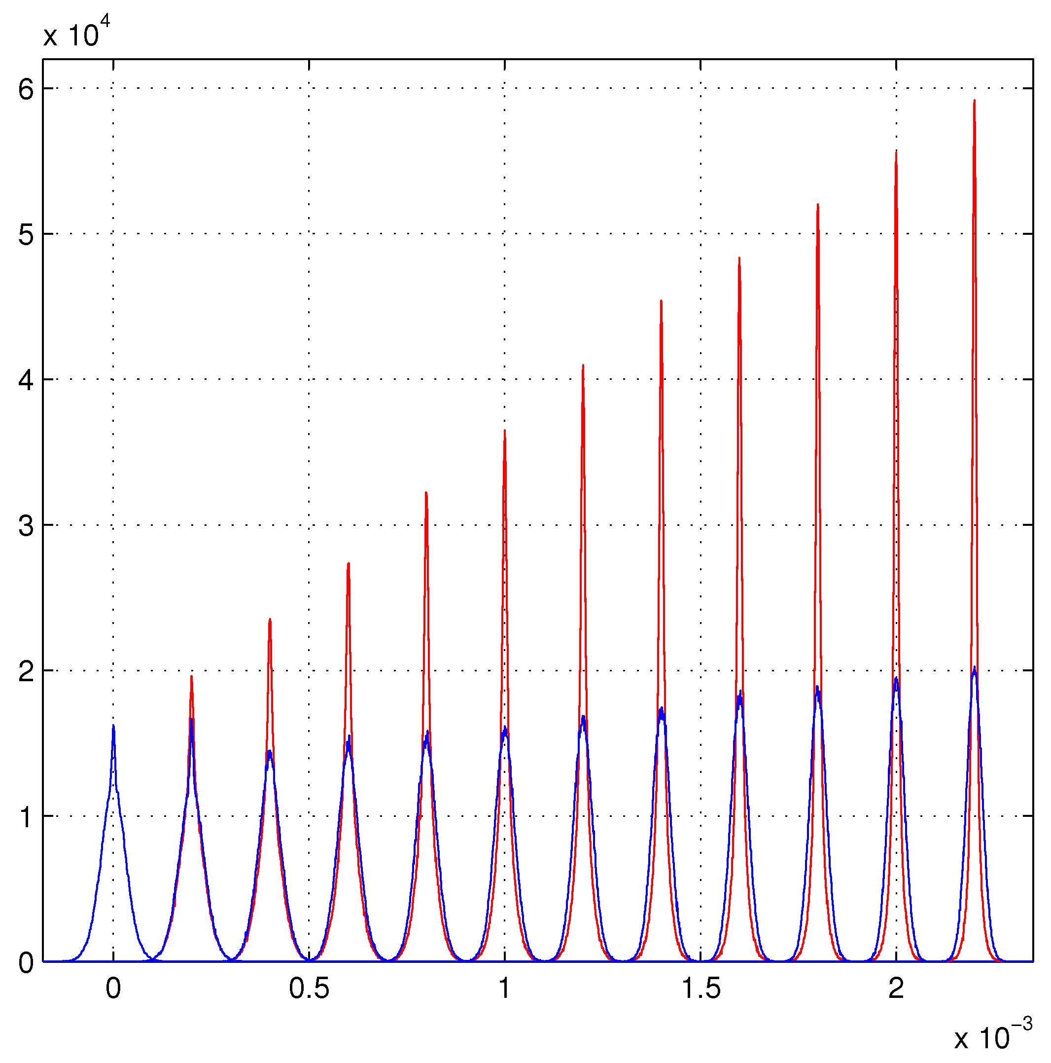Figure 1 illustrates these limits for the $\gamma$ estimator (the blue distributions) also ${\sum }_j{y}_j^2$ cannot grow faster than N for the fixed length of the tracker. The large modifications of the variances of the chains of PDFs, render the track fitting strongly dependent from other PDFs. For example, those that select the chains among the possible set of chains. These PDFs are introduced by the properties of the measuring devices. As we said above, a binomial PDF suffices in the disordered tracker detector for the models of refs. [2,3], just a mean disorder of half strip (≈30 $\mathsf{\mu }$m) is enough for this. The use of standard least-squares method in heteroscedastic models has enormous simplifications, because it does not need the knowledge of the ${\sigma }_j$ for each observation. Unfortunately, it amounts to a large loss of resolution. Our models of ref. [3] illustrate in evident way the amplitude of this loss. In any case the lucky model of ref. [3] can be an economic way to introduce effective ${\sigma }_j$.

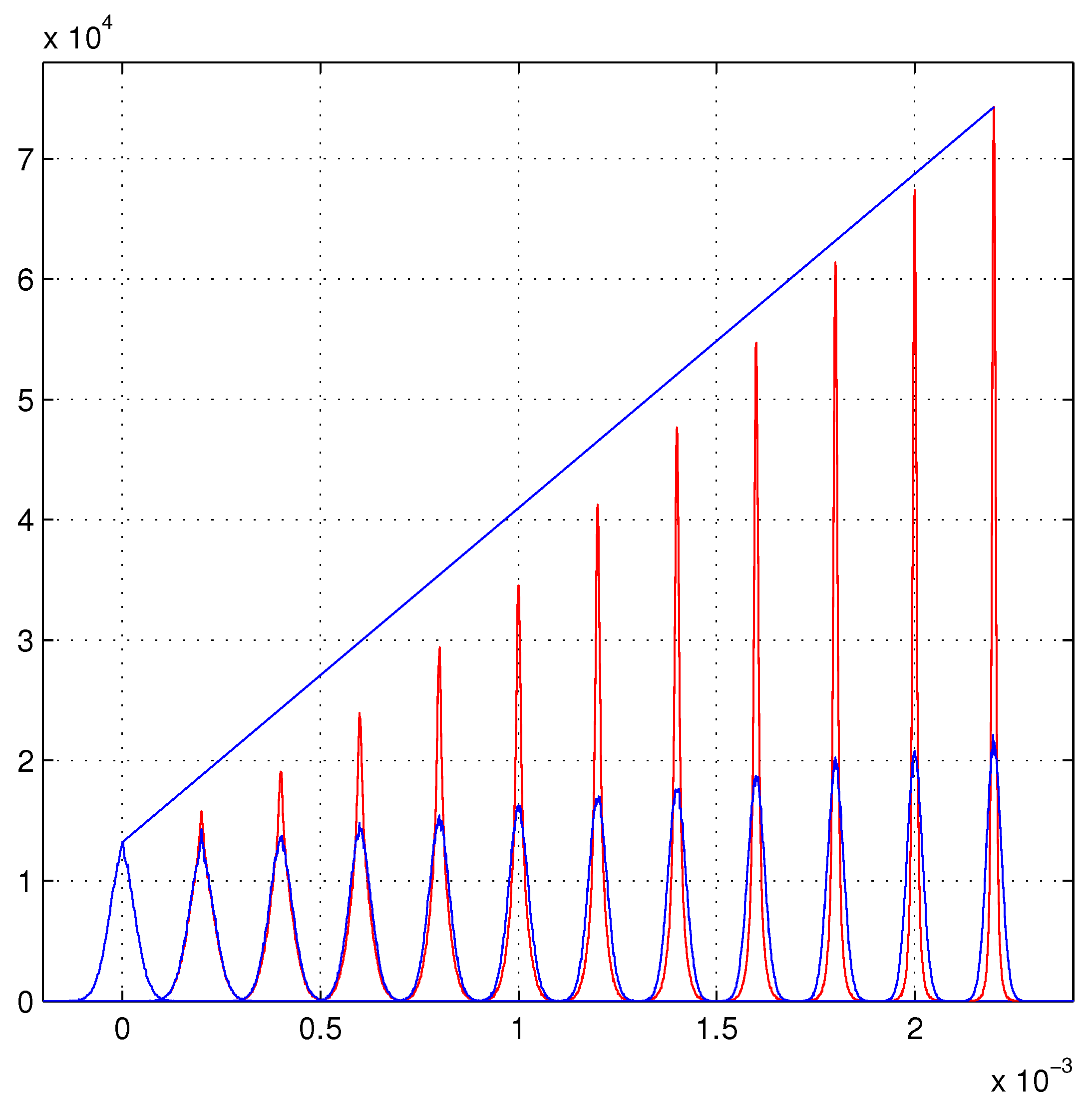
For our pleasure, in Figure 2, we invented a faster growth than that of the Gaussian model of ref. [3]. The quality of the detectors increases with the number N of detecting layers, each inserted layer is better than the previous one. The bleu straight line shows an evident deviation from a linear growth with an almost parabolic growth (with the variances going down as $1/N^4$). The blue distributions are practically insensible to these changes. With appropriate selection of the detector quality many types of growth can be implemented.

4.2. Deviations from Optimality

Equations (41) prove the non-optimality of the standard least-squares in the case of its use with a different (heteroscedastic) likelihood. The standard least squares is the efficient estimator for a homoscedastic Gaussian model, the use outside this condition of efficiency (optimality) destroys its optimality and produces an increase of variances with a degradation of the resolution, as illustrated by the simulations of ref. [1,2,3]. Even our heteroscedastic model suffers of a similar optimality loss outside its range of validity. We underlined that the orders and the values (whatever they are) of the set of $\left\{{\sigma }_j\right\}$, in the likelihood, define the model. Each deviation from the values or the order (or both) of the ${\sigma }_j$ implies an increase of the variance of the new estimator compared to the variance of the optimal (efficient) estimator. We used this property to prove the crucial correlation of the appropriate ${\sigma }_j$ with the hit j. If the ordered set of $\left\{{\sigma }_j\right\}$ is randomized, destroying the correlation with the set of the hits, the distributions of the estimators change drastically becoming worse than the standard least-squares. Instead, the differences of the heteroscedastic efficient estimator minus suboptimal estimators, with the elimination of some PDFs, rapidly converge toward zero when the suppressed PDFs are reduced. This rapid convergence is not observed in the case of the standard least-squares.

5. Inequality for Momentum Estimators

As anticipated above, the CRF-inequality will be extended to case of the momentum reconstruction. It will be studied the case of a high-momentum charged particle moving in a tracker with a homogeneous magnetic field and the path of the particle orthogonal to the field direction. Here, the segment of the circular path can be approximated with a parabolic path (algorithms for circular path are described in ref. [10]). As for the straight tracks, we will compare the estimators of standard least squares with those of a heteroscedastic model. The estimators of the standard least-squares are efficient (optimum) in the homoscedastic Gaussian model.

5.1. The Momentum Estimators in Homoscedastic Gaussian Model

We use this approach to define our expressions for the estimators. These forms will be used in heteroscedastic models. Our equation will be expressed in compact way with matrices. The function $\mathfrak{L}(\mathbf{x},\beta ,\gamma ,\eta )$ is the likelihood for this case, $\beta$ and $\gamma$ are just defined, $\eta$ is the curvature of the track, proportional to $1/p$ with p the track momentum:

$$\begin{array}{c}\mathfrak{L}(\mathbf{x},\beta ,\gamma ,\eta )=f_1(x_1,\beta ,\gamma ,\eta )f_2(x_2,\beta ,\gamma ,\eta )\dots f_N(x_N,\beta ,\gamma ,\eta )\hfill \\ f_j(x,\beta ,\gamma ,\eta )=\frac{exp[-{(x-\beta -\gamma y_j-\eta y_j^2)}^2/2{\sigma }^2]}{\sqrt{2\pi }\sigma }\hfill \end{array}$$

(42)

The index j orders the PDFs $f_j$ as the tracker layers. The equivalent of Equation (27) is:

$$V(\mathbf{x},\beta ,\gamma ,\eta )=\left(\begin{array}{c}{\displaystyle \frac{\partial ln\mathfrak{L}(\mathbf{x},\beta ,\gamma ,\eta )}{\partial \beta }}\\ {\displaystyle \frac{\partial ln\mathfrak{L}(\mathbf{x},\beta ,\gamma ,\eta )}{\partial \gamma }}\\ {\displaystyle \frac{\partial ln\mathfrak{L}(\mathbf{x},\beta ,\gamma ,\eta )}{\partial \eta }}\end{array}\right)$$

(43)

The unbiased estimators for $\beta ,\gamma ,\eta$ are obtained from $V(\mathbf{x},\beta ,\gamma ,\eta )$:

$$V(\mathbf{x},\beta ,\gamma ,\eta )=\left(\begin{array}{c}{T}_a\left(\mathbf{x}\right)\\ T_b\left(\mathbf{x}\right)\\ T_c\left(\mathbf{x}\right)\end{array}\right)-\mathbf{R}\left(\begin{array}{c}\beta \\ \gamma \\ \eta \end{array}\right) {\mathbf{R}}^{-1}V(\mathbf{x},\beta ,\gamma ,\eta )={\mathbf{R}}^{-1}\left(\begin{array}{c}{T}_a\left(\mathbf{x}\right)\\ T_b\left(\mathbf{x}\right)\\ T_c\left(\mathbf{x}\right)\end{array}\right)-\left(\begin{array}{c}\beta \\ \gamma \\ \eta \end{array}\right)$$

(44)

The vector ${\mathbf{R}}^{-1}V(\mathbf{x},\beta ,\gamma ,\eta )$ contains the efficient estimators of this model, the matrix $\mathbf{R}$ is its Fisher information (with the condition ${\sum }_j{y}_j=0$ and $j=\{1,2,\dots ,N\}$):

$$\mathbf{R}=\left(\begin{array}{ccc}N\hfill & 0\hfill & {\sum }_j{y}_j^2\hfill \\ 0\hfill & \sum _j{y}_j^2\hfill & \sum _j{y}_j^3\hfill \\ \sum _j{y}_j^2\hfill & \sum _j{y}_j^3\hfill & \sum _j{y}_j^4\hfill \end{array}\right)\frac{1}{{\sigma }^2} .$$

(45)

For Equation (35) extended to this case, it is:

$$\begin{array}{c}\int V(\mathbf{x},\beta ,\gamma ,\eta )·V^{\prime }(\mathbf{x},\beta ,\gamma ,\eta ) \mathfrak{L}(\mathbf{x},\beta ,\gamma ,\eta )\mathrm{d}\mathbf{x}=\mathbf{R}\hfill \\ \int {\mathbf{R}}^{-\mathbf{1}}V(\mathbf{x},\beta ,\gamma ,\eta )·V^{\prime }(\mathbf{x},\beta ,\gamma ,\eta ){\mathbf{R}}^{{-\mathbf{1}}^{\prime }} \mathfrak{L}(\mathbf{x},\beta ,\gamma ,\eta )\mathrm{d}\mathbf{x}={\mathbf{R}}^{-\mathbf{1}} .\hfill \end{array}$$

(46)

The matrices $\mathbf{R}$ and ${\mathbf{R}}^{-\mathbf{1}}$ are symmetric and positive semi-definite. The second line of the last equation is the variance-covariance matrix of the efficient estimators. The variance-covariance matrix of a generic vector T of unbiased estimators of $\beta ,\gamma ,\eta$ with the efficient estimators is:

$$\mathbf{K}=\left(\begin{array}{cc}<T T^{\prime }>& <T V^{\prime }{\mathbf{R}}^{{-\mathbf{1}}^{\prime }}>\\ <{\mathbf{R}}^{-\mathbf{1}}V T^{\prime }>& {\mathbf{R}}^{-\mathbf{1}}\end{array}\right)\ge 0$$

(47)

As defined, the symbol $< >$ indicates an integral with the likelihood $\mathfrak{L}$. The cross correlations $<V T^{\prime }>$ follow the rules of Equation (39) giving now the $3x3$ identity matrix ${\mathbb{I}}_3$ reducing the off-diagonal elements of $\mathbf{K}$ to ${\mathbf{R}}^{-1}$. With a transformation of the type ${\mathbf{A}}^{\prime } \mathbf{K} \mathbf{A}$ with a $6x3$ real matrix $\mathbf{A}$ the fundamental inequality is obtained:

$$({\mathbb{I}}_3 -{\mathbb{I}}_3)\left(\begin{array}{cc}<T T^{\prime }>& {\mathbf{R}}^{{-\mathbf{1}}^{\prime }}\\ {\mathbf{R}}^{-\mathbf{1}}& {\mathbf{R}}^{-\mathbf{1}}\end{array}\right)\left(\begin{array}{c}{\mathbb{I}}_3\\ -{\mathbb{I}}_3\end{array}\right)=\langle T T^{\prime }\rangle -{\mathbf{R}}^{-\mathbf{1}}\ge 0$$

(48)

The equality is obtained only for the efficient estimators of this model. Therefore, any other set of estimators have a greater variance in this model. Any heteroscedastic model has greater variance than the efficient model. The reason is connected to the modification that the likelihood $\mathfrak{L}$ introduces in the variances. These modifications always increase the variances. In this model, the parameter $\sigma$ disappears in the expressions for the estimators. The form $\mathbf{R}$ of the Fisher information depends from N, this limits the growth with the numbers of detecting layers as illustrated in ref. [2].

5.2. The Momentum Estimators in Heteroscedastic Gaussian Model

In its essence this model can be obtained from the corresponding homoscedastic model with a set of formal differences.

$$\begin{array}{c}L(\mathbf{x},\beta ,\gamma ,\eta )=f_1(x_1,\beta ,\gamma ,\eta )f_2(x_2,\beta ,\gamma ,\eta )\dots f_N(x_N,\beta ,\gamma ,\eta )\hfill \\ f_j(x,\beta ,\gamma ,\eta )=\frac{exp[-{(x-\beta -\gamma y_j-\eta y_j^2)}^2/2{\sigma }_j^2]}{\sqrt{2\pi }{\sigma }_j}\hfill \end{array}$$

(49)

The index j orders the PDFs as the detecting layers and selects a different ${\sigma }_j$ for this observation. The other differences are in the definitions of the vector $T_1,T_2,T_3$ that are different from the previous $T_a,T_b,T_c$ and the Fisher information $\mathbf{I}$.

$$U(\mathbf{x},\beta ,\gamma ,\eta )=\left(\begin{array}{c}{T}_1\left(\mathbf{x}\right)\\ T_2\left(\mathbf{x}\right)\\ T_3\left(\mathbf{x}\right)\end{array}\right)-\mathbf{I}\left(\begin{array}{c}\beta \\ \gamma \\ \eta \end{array}\right) \left(\begin{array}{c}{T}_1\left(\mathbf{x}\right)\\ T_2\left(\mathbf{x}\right)\\ T_3\left(\mathbf{x}\right)\end{array}\right)=\left(\begin{array}{c}{\sum }_j\frac{x_j}{{\sigma }_j^2}\\ {\sum }_j\frac{x_j y_j}{{\sigma }_j^2}\\ {\sum }_j\frac{x_j y_j^2}{{\sigma }_j^2}\end{array}\right)$$

(50)

The Fisher information becomes:

$$\mathbf{I}=\left(\begin{array}{ccc}\sum _{j}1/{\sigma }_j^2\hfill & \sum _j{y}_j/{\sigma }_j^2\hfill & \sum _j{y}_j^2/{\sigma }_j^2\hfill \\ \hfill & \hfill \\ \sum _j{y}_j/{\sigma }_j^2\hfill & \sum _j{y}_j^2/{\sigma }_j^2\hfill & \sum _j{y}_j^3/{\sigma }_j^2\hfill \\ \hfill & \hfill \\ \sum _j{y}_j^2/{\sigma }_j^2\hfill & \sum _j{y}_j^3/{\sigma }_j^2\hfill & \sum _j{y}_j^4/{\sigma }_j^2\hfill \end{array}\right)$$

(51)

The efficient unbiased estimators for the likelihood $L(\mathbf{x},\beta ,\gamma ,\eta )$ are contained in the vector ${\mathbf{I}}^{-\mathbf{1}}U(\mathbf{x},\beta ,\gamma ,\eta )$. Even in this case the Fisher information has no obvious N-dependence. The variance- covariance matrix for any vector T (as T = $(T_a ,T_b ,T_c)$) with the unbiased estimators can be transformed as described giving the inequality:

$$({\mathbb{I}}_3 -{\mathbb{I}}_3)\left(\begin{array}{cc}<T T^{\prime }>& {\mathbf{I}}^{{-\mathbf{1}}^{\prime }}\\ {\mathbf{I}}^{-\mathbf{1}}& {\mathbf{I}}^{-\mathbf{1}}\end{array}\right)\left(\begin{array}{c}{\mathbb{I}}_3\\ -{\mathbb{I}}_3\end{array}\right)=\langle T T^{\prime }\rangle -{\mathbf{I}}^{-\mathbf{1}}\ge 0$$

(52)

The symbol $< >$ indicates an integral on $\mathbf{x}$ with the likelihood of this model $L(\mathbf{x},\beta ,\gamma ,\eta )$. The equality to zero is obtained only when the vector T is ${\mathbf{I}}^{-\mathbf{1}}U(\mathbf{x},\beta ,\gamma ,\eta )$. For any other unbiased estimator, that difference is greater than zero (in the sense of the positive semi-definite matrices).

These last forms of demonstration easily extend the CRF-inequality to any number M of estimators.

6. Conclusions

The Cramer–Rao–Frechet inequality is applied to a set of heteroscedastic Gaussian model to prove the absence of any limitation introduced by this fundamental inequality. Instead, the inequality shows that in heteroscedastic models, the estimators of the standard least-squares have always greater variances compared to that given by the weighted least-squares. The variances of the standard least-squares conserve approximate $1/\mathrm{N}$ form that imply limitations in the growth of the distributions with the number $\mathrm{N}$ of detecting layers. No similar limitations are present in the weighted least-squares that are dominated by the differences of the weights $1/{\sigma }_j^2$. For identical ${\sigma }_j$ the estimators converge to those of the standard least-squares. The inequality is calculated also for the momentum estimators. Again the appropriate heteroscedastic estimators have a lower variance than those of the standard least-squares. Given the loss of resolution implied by greater variances, it must be avoid the use of standard least-squares with heteroscedastic data. The lucky model may be helpful in silicon detectors to insert the approximate ${\sigma }_j$ to each observation.

References

1. Landi, G.; Landi, G.E. Improvement of track reconstruction with well tuned probability distributions. J. Instrum. 2014, 9, P10006. [Google Scholar] [CrossRef] [Green Version]
2. Landi, G.; Landi, G.E. Optimizing momentum resolution with a new fitting method for silicon-strip detectors. Instruments 2018, 2, 22. [Google Scholar] [CrossRef] [Green Version]
3. Landi, G.; Landi, G.E. Beyond the N -limit of the least squares resolution and the lucky-model. arXiv 2018, arXiv:1808.06708. [Google Scholar]
4. Anonymous editor and referee of a journal of instrumentation. Private written communications, 2019.
5. Ito, S.; Dechant, A. Stochastic time evolution, information geometry and Cramer-Rao bound. arXiv 2018, arXiv:1810.06832. [Google Scholar]
6. Ivchenko, G.; Yu, M. Mathematical Statistics; URSS: Moscow, Russia, 1990. [Google Scholar]
7. Gowan, G. Statistical Data Analisis; Oxford University Press: Oxford, UK, 1998. [Google Scholar]
8. Olive, K.A.; Agashe, K.; Amsler, C.; Antonelli, M.; Arguin, J.-F.; Asner, D.M.; Baer, H.; Band, H.R.; Barnett, R.M.; Basaglia, T.; et al. Particle Data Group. Chin. Phys. C 2014, 38, 090001. [Google Scholar] [CrossRef]
9. Amemiya, T. Advanced Econometrics; Harvard University Press: Cambridge, MA, USA, 1985. [Google Scholar]
10. Al-Sharadqah, A.; Chernov, N. Error analysis for circle fitting algorithms. Electron. J. Stat. 2009, 3, 886–911. [Google Scholar] [CrossRef]
11. MATLAB 8; The MathWorks Inc.: Natick, MA, USA, 2012.
Figure 1. Empirical PDFs of the fitted (straight) track direction for tracker models with N = 2 to N = 13 detecting layers. The PDFs for N = 2 are centered on zero, the others are shifted by N-2 steps of fixed amplitude. The blue PDFs are the results of the standard least-squares. The red PDFs are obtained with the weighted least-squares. (The reported dimensions are pure numbers).
Instruments 04 00002 g001
Figure 2. Another Gaussian model. A faster increase in the maximums compared to that of Figure 1. The blue straight lines connect the maximum of the first distribution to that of the last red distribution. The color cade is that of Figure 1.
Instruments 04 00002 g002