Article

Optimizing Momentum Resolution with a New Fitting Method for Silicon-Strip Detectors

by
Gregorio Landi
1,* and
Giovanni E. Landi
2
1
Department of Physics and Astronomy, University of Firenze, and INFN, Largo E. Fermi 2 (Arcetri), 50125 Firenze, Italy
2
ArchonVR S.a.g.l., Via Cisieri 3, 6900 Lugano, Switzerland
*
Author to whom correspondence should be addressed.
Instruments 2018, 2(4), 22; https://doi.org/10.3390/instruments2040022
Submission received: 1 September 2018 / Revised: 20 October 2018 / Accepted: 30 October 2018 / Published: 31 October 2018

Abstract

:
Two new fitting methods are explored for momentum reconstruction. They give a substantial increase of momentum resolution compared to standard fit. The key point is the use of a different (realistic) probability distribution for each hit (heteroscedasticity). In the first fitting method an effective variance is calculated for each hit, the second method uses the search of the maximum likelihood. The tracker model is similar to the PAMELA tracker with its two sided detectors. Here, each side is simulated as a momentum reconstruction device. One of the two is similar to silicon micro-strip detectors of large use in running experiments. The gain obtained in momentum resolution is measured as the virtual magnetic field and the virtual signal-to-noise ratio required by the standard fits to overlap with the best of the new methods. For the low noise side, the virtual magnetic field must be increased 1.5 times to reach the overlap and 1.8 for the other. For the high noise side, the increases must be 1.8 and 2.0. The signal-to-noise ratio has to be increased by 1.6 for the low noise side and 2.2 for the high noise side ( η -algorithms). Each one of our two methods shows a very rapid linear increase of the resolution with the number N of detector layers, the two standard fits have the usual slow growth less than N .

1. Introduction

Momenta of charged particles are fundamental pieces of information in high energy particle physics. For their acquisition, very complex instruments (trackers) have been developed and the key element of a tracker is a uniform (or near to) magnetic field. In a homogeneous magnetic field a free charged particle describes an helicoidal path, the radius of the helix is proportional to the momentum component orthogonal to the magnetic field. The chirality of the helix is given by the sign of the charge. The precise reconstructions of these non linear paths allow the trackers to measure the particle momenta and to fix the charge signs. Various effects deviate the particle tracks from their theoretical forms and refined methods must be introduced to account for these deviations and limit the measurement degradations. Among the degrading effects we quote the multiple (Coulomb) scattering, the energy loss, the inhomogeneities of the magnetic field and the systematic and statistical errors of the positioning algorithms. Recent papers [1,2] (to mention the most recent ones of a very large set) address the first three effects. The handling of the full non linearity of the particle path is described in ref. [3].
This work addresses studies of the statistical effects in the positioning algorithms of minimum ionizing particle (MIP) and how to minimize their influence in the momentum reconstruction. For this task, realistic probability density functions (PDFs; probability distributions in the physicist jargon) for the errors of the positioning algorithms must be used. This strategy allows going beyond the results of the standard least squares method or other fitting methods that neglect the differences of the statistical properties of the hits, or the heteroscedasticity (as it is called in statistics). For our task, we will simulate momentum values where the multiple scattering is negligible, similarly for the energy loss (principally for electrons) and the magnetic inhomogeneities. The systematic errors in the positioning algorithms are unavoidable and must be accounted properly. The center of gravity (COG in the following) as a positioning algorithm was detailed discussed in refs. [4,5] where exact analytical forms were demonstrated for its systematic error. Due to its (apparent) simplicity the COG is one of the most used positioning algorithms: x g = j x j τ j / j x j , where x j and τ j are the signals and the positions used. Even if a single name is used for the COG, slight different version are in use. The principal differences are in number of signal used, each selection implies different analytical properties and different systematic errors. The differences of each COG-version are quite evident in our approach, the realistic PDFs show very different analytical forms and statistical properties. To keep track of these differences we will indicate with COG n a COG algorithm with n-strips. Due to these different forms and properties, a rigid distinction must be exercised among the various COG n algorithms and the best one must be used for each condition. The developments of ref. [4] and the mathematical approaches explored there for the COG study are very complex, but these complexities are typical of the fight against the systematic errors. For example, Gauss demonstrated what he called “Theorema Egregium” for the systematic errors of his topographic maps, and the recommendations on the systematic error suppression are always preliminary statements in his papers on least squares [6]. With heteroscedasticity as a basic assumption, Gauss papers [6] deviate in an essential way from the standard expositions of the least squares method, those simplifications (often presented as Gauss-Markov theorem) surely generate many suboptimal fits in physical applications.
An interesting achievement, to suppress the COG 2 systematic error, was reported in ref. [7] i.e., the η -algorithm. A preliminary assumption of the method is the uniform “illumination” of the strips by MIP signals from parallel incidence. In this case, the non uniform distribution of the COG 2 , given by systematic error, can be reduced to a uniform one. As clearly stated by the authors, the derivation of ref. [7] is limited to symmetric signal distributions collected by the two (adjacent) leading strips of a cluster. It is evident that for inclined tracks or in presence of a magnetic field the symmetry, if present at orthogonal incidence, is surely destroyed. To overcome these limitations, the analytic methods developed in ref. [4] were essential. They were used in ref. [8] to generalize the η -algorithm beyond the two strip limitation and to extract the required corrections for non symmetric configurations. The set of generalizations will be indicated as η n -algorithm, where the index n is connected to the number of strips contained in the COG n algorithm from which the η algorithm is derived. Here, we will use always the COG 2 and the η 2 -algorithm. At our orthogonal incidence, the signals collected by the two leading strips suffice for the reconstructions.
The fit of straight tracks was the first problem we faced with this new fitting method, even if the straight tracks are not the principal task in high energy physics. The results obtained were described in ref. [9]. The limitation to straight tracks was mainly due to the complexity of the method we applied for the first time. Hence, working with two parameters, the debugging and testing of the maximum likelihood application can be followed on a surface. Furthermore, the data, elaborated in our approach, were collected in a CERN test beam [10] in the absence of a magnetic field. The detectors, that we used, were a few samples of double-sided silicon micro-strip detectors [11,12] as those making up the PAMELA tracker [13]. The results of ref. [9] showed a drastic improvement of the fitted track parameters in comparison to the results of the least squares methods. We observed excellent reconstructions even in presence of very noisy hits, often called outliers, that generally produce bad fits. This achievement is almost natural for the heavy tails of our non gaussian PDFs . On the contrary, the least squares method, being strictly optimum for a gaussian PDF, must be modified in a somewhat arbitrary way to handle these pathological (for a gaussian PDF) hits, often with scarce or no result.
We have to recall that the perception of a rough handling of the hit PDFs is well present in literature, and Kalman-filter modifications are often studied to accept extended deviations from a pure Gaussian model. These extensions use linear combinations of different Gaussians [14,15], the number of them is limited to avoid the intractability of the equations. The unknown parameters are selected from an optimization of the fit results. In a broad sense, our schematic approximations could be reconnected to those extensions. In fact, to speed the convergence of the maximum likelihood search, we calculate an effective variance for each hit and use this variance in a weighted least squares.
The confidence gained in ref. [9] with straight tracks allow us to deal with more complex and appealing tasks, i.e., the reconstruction of tracks in a magnetic field and the measure of their momenta. To face this extension with the minimum modifications of our previous work, and saving a backward compatibility, we will use the simulated data and parameters used in ref. [9] thus this reference will be often quoted as a repository of details not reported here. Now those data are adapted to the PAMELA geometry and to a constant magnetic field of 0.44 T near to the average field of the PAMELA tracker. This relatively low magnetic field introduces small modifications of the parameters obtained in its absence. The average signal distribution of a MIP is slightly distorted by a Lorentz angle, that, in the present conditions, is about 0.7 . Around this incidence angle, the average signal distribution of a MIP is practically identical to that at orthogonal incidence in the absence of a magnetic field. Thus, without further notice, we will assume a rotation of the detectors of their Lorentz angle with respect to our MIP direction. These assumptions allow to use our previously generated data and to simulate high momentum tracks for each side of the double sided detectors. In the PAMELA tracker, the low noise side of the detector is used for momentum measurements. This side has an excellent resolution due to its special structure. A strip each two is connected to the read out system, the unconnected strip distributes the incident signal on the nearby strips optimizing the detector resolution (floating strip side). The other side (normal noisy side) is devoted to the reconstruction of the straight part of a track, it has the strips oriented perpendicularly to the other side. Each strip is connected to the readout system and has, by the complexity of construction, a higher noise and a small, if any, signal spread to nearby strips. For this last characteristic, this side responds in a way similar to the types of microstrip arrays used in the large trackers of the CERN LHC [16,17,18]. The simulations on this side, as bending side, can give a glimpse of our approach for other type of trackers even for the (small angle stereo) double-sided detectors of the ALICE [16] experiment. For these reasons, this side will be indicated as normal noisy side.
In Section 2, a few details of this new fitting method will be recalled with a derivation of the general probability distribution. Section 3 and Section 4 are devoted to the momentum PDF for the each side of this two sided detectors. In Section 5 the results of the simulations will be discussed and related to physical properties of the detection system. Section 6 summarizes the results. A partial preliminary version of this paper was reported in [arXiv:1606.03051].

2. Details of the Method

The possibility of different statistical properties of each hit is based on well known properties of the MIP hitting a silicon strip (or gas discharge) detectors, largely reported in literature: (a) the charge released in each hit has a Landau distribution with different signal-to-noise ratio. (b) The position resolution depends from the charge spreading thus it is better near to the strip border (e.g., ref. [19] for gas ionization chambers) (c) Each strip has its own noise. Thus, the assumption of homoscedasticity (on an entire detector layer) is inconsistent for the previous well known reasons, which are common to a large class of detectors. Even if the hit properties (a)–(c) are well known, no attempt was done to insert them in a fit for the mathematical difficulties of this task. For the first time, we developed a set of analytical tools to insert these random effects in track reconstruction. The complex mathematical infrastructure, we realized, is able to generate appropriate PDF for each hit, hundreds of thousands of different PDFs. A few results of this mathematical infrastructure, illustrated in the follow, are reported in Figure 1. They are samples of the (calculated) effective variances [9] for hits in the two sides of our micro-strip detectors. Small effective variances at the strip borders can be observed in the right part of Figure 1 for the noisy normal strip side. They share some similarity with the results of ref. [19] supporting a general aspect of this border effect. The floating strip side is almost always much better, the vertical scale of the right plot is around three times that of the left plot. Even this side shows a border effect similar to the other side, here the physical border of the readout strip is at ± 0.25 .
The demonstration of different PDF for groups of hits, or as in our case a different PDF for each hit, poses serious problems to the use the standard least squares as a fitting tool. A frequently used assumption to derive the least squares (or linear regression as it is often called) properties is the identity of the variance of the (hit) measurement errors (homoscedasticity) and a horizontal line of dots in each side of Figure 1. In this case, it is easy to show the optimality and the unbiasedness of the method. If the homoscedasticity breaks down, the optimality and unbiasedness disappear. Linearity is the only surviving feature. It must be clear that the loss of the optimality means a loss in resolution, and resolution is our fundamental aim. Similar warnings must be raised for the detector architectures simulated (and realized) starting from non-optimal methods. The benefit of this trivialization of the Gauss approach [6], where heteroscedasticity is assumed from the very beginning, it is unclear.

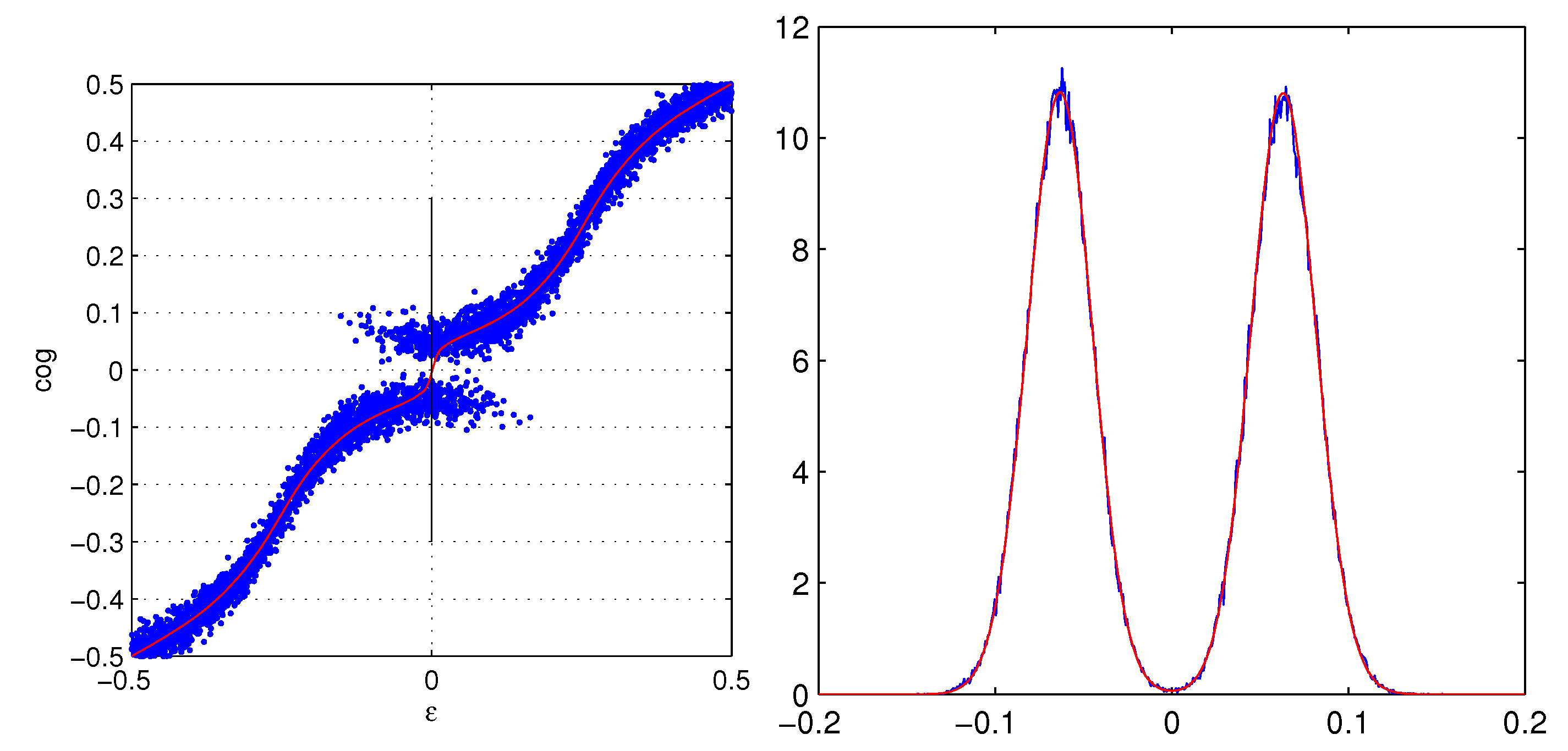
2.1. A Short Derivation of the PDF for the COG 2 Algorithm

The incidence angle of our MIPs imposes the use of the minimum number of signal strips to reduce the noise, hence, as stated above, only two signal strips will be used. In ref. [9] we indicated the principal steps required to obtain the PDF for the COG 2 (two-strip COG), those steps followed the standard method described in the books about the theory of probability. At first one has to obtain the cumulative distribution with integrations on complex surfaces, after, the derivative of the cumulative distribution gives the PDF. The length and the complexity of this development (our first procedure) is not suitable for publication. A simpler and more direct method applied to a few COG n algorithms will be published elsewhere. A small portion of that method is reported here. In a few steps, results identical to those given by the cumulative distribution are obtained. Here, the COG 2 algorithm has the origin of its reference system in the center of the maximum-signal strip. The strip signals are indicated with: x 1 , x 2 , and x 3 , respectively the signal of the right strip, central strip (with the maximum signal) and left strip. If x 1 > x 3 the COG 2 is x = x 1 / ( x 1 + x 2 ) , if x 3 > x 1 it is x = x 3 / ( x 3 + x 2 ) . Thus the probability P x g 2 of COG 2 to be x is given by:
P x g 2 ( x ) = + d x 1 d x 2 d x 3 P ( x 1 , x 2 , x 3 ) θ ( x 1 x 3 ) δ ( x x 1 x 1 + x 2 ) + θ ( x 3 x 1 ) δ ( x + x 3 x 3 + x 2 )
where P ( x 1 , x 2 , x 3 ) is the PDF to have the signals x 1 , x 2 , x 3 from the strips 1 , 2 , 3 . The signals x i are at their final elaboration stage (pedestals, common noise, etc.) and ready to be used for the hit-position reconstruction. The function θ ( x j ) is the Heaviside θ -function: θ ( x j ) = 1 for x j > 0 , θ ( x j ) = 0 for x j 0 , and δ ( x ) is the Dirac δ -function. The normalization of P x g 2 ( x ) can be easily verified by an integration on x. Equation (1) can be further elaborated with the following transformations. Splitting the sum of Equation (1) in two independent integrals and transforming the variables x 1 = ξ , x 1 + x 2 = z 1 and x 3 = β , x 3 + x 2 = z 2 , the Jacobian of the transformation is one and the integrals in z 1 and z 2 can be performed with the rule:
+ d z F ( z ν ) δ ( x ν z ) = F ( ± ν x ν ) | ν | x 2 .
Applying Equation (2) to Equation (1) and using the limitations of the two θ -functions, Equation (1) becomes:
P x g 2 ( x ) = 1 x 2 [ + d ξ ξ d β P ξ , ξ 1 x x , β | ξ | + + d β β d ξ P ξ , β 1 x x , β | β | ] .
This form underlines very well the similarity with the Cauchy PDF; in the limit of x the x-part of the P ( . ) arguments are 1 and P x g 2 ( x ) 1 / x 2 for large x.

2.2. The Probability P x g 2 ( x ) for Small x

The probability P ( x 1 , x 2 , x 3 ) can handle a strict correlation among its arguments, we abandon this strict correlation with the weakest one: the mean values of the strip signals { a i } are correlated, but the fluctuations around { a i } are independent. Thus the probability P ( x 1 , x 2 , x 3 ) becomes the product of three functions { P i ( x i ) , i = 1 , 2 , 3 } . Each P i ( x i ) is assumed to be a gaussian PDF with mean values a i and standard deviation σ i (the strip additive noise is well reproduced by a gaussian PDF in the absence of MIP signals). To simplify, the constants a i , i = 1 , 2 , 3 are the noiseless signals released by a MIP with impact point ε :
P i ( x i ) = exp ( x i a i ) 2 2 σ i 2 1 2 π σ i .
Even with the gaussian functions, the integrals of Equation (3) have no analytical expressions and effective approximations must be constructed. We will not report our final forms that are very long, instead we will illustrate a limiting case which gives a simple approximation and eliminates a disturbing singularity for the numerical integrations. It is easy to show that for | x | 0 , x 1 P 2 ξ ( 1 x ) / x and x 1 P 2 β ( 1 x ) / x converge to two Dirac δ -functions. Hence, for small | x | (or better for | x | σ 2 / a 2 1 ), the integrals of Equation (3) can be expressed as:
P x g 2 ( x ) = | a 2 | 2 π { exp ( x a 1 a 1 + a 2 ) 2 ( a 1 + a 2 ) 2 2 σ 1 2 ( 1 x ) 2 1 erf ( a 3 a 2 + a 3 x ) a 2 + a 3 2 σ 3 | 1 x | 2 σ 1 ( 1 x ) 2 + exp ( x + a 3 a 3 + a 2 ) 2 ( a 3 + a 2 ) 2 2 σ 3 2 ( 1 + x ) 2 1 erf ( a 1 a 2 + a 1 + x ) a 2 + a 1 2 σ 1 | 1 + x | 2 σ 3 ( 1 + x ) 2 } .
Equation (5) is correct for | x | 0 , but it is useful beyond this limit, as far as the pole for x = ± 1 is irrelevant, and it contains many ingredients of more complex expressions.
An example of Equation (5) can be seen in the right side of Figure 2. The essential elements are the two maxima (gaussian-like) centered in the possible noiseless two-strip COG: a 1 / ( a 1 + a 2 ) and a 3 / ( a 3 + a 2 ) . The widths of the two maxima are modulated by the signal-to-noise ratio ( a 2 + a 1 ) / σ 1 and ( a 2 + a 3 ) / σ 3 , the 1 ± x factor is relevant at the borders of the x-range, i.e., x = ± 0.5 . Each maximum has a scaling factor | a 2 | / σ 1 or | a 2 | / σ 3 that, for the large majority of strip clusters σ 1 σ 2 σ 3 , is the signal to noise ratio of the central strip.
Increasing the impact position ε , the lowest maximum tends to disappear. Similarly at decreasing ε , the highest maximum is rapidly reduced. The tails of the maxima differ drastically from gaussian PDF. More complete expressions of Equation (5) contain terms very similar to Cauchy PDFs, they have no a j factors and survive when all the a j are zero.
The dimensions of the constants a j must be those of the σ j , for both of them we take directly the ADC counts. The x-variable (the COG 2 ) is a pure number expressed as a fraction of the strip width, or more precisely, the strip width is the scale of lengths. In the simulated distribution of Figure 2, the particle track is split in 15 segment and each segment has a different ionization density, obtained from a Landau PDF accorded to the length of the segment. The total ionization is normalized to a constant value. The ionization of each segment is independently diffused toward the collecting strips and scaled to the signal mean value, a gaussian noise of 4 ADC counts is added to each strip. The distribution of the COG 2 is reported in the normalized histogram, and it shows that, at this orthogonal incidence. the Landau fluctuations are well represented by the fluctuations of the total collected charge.

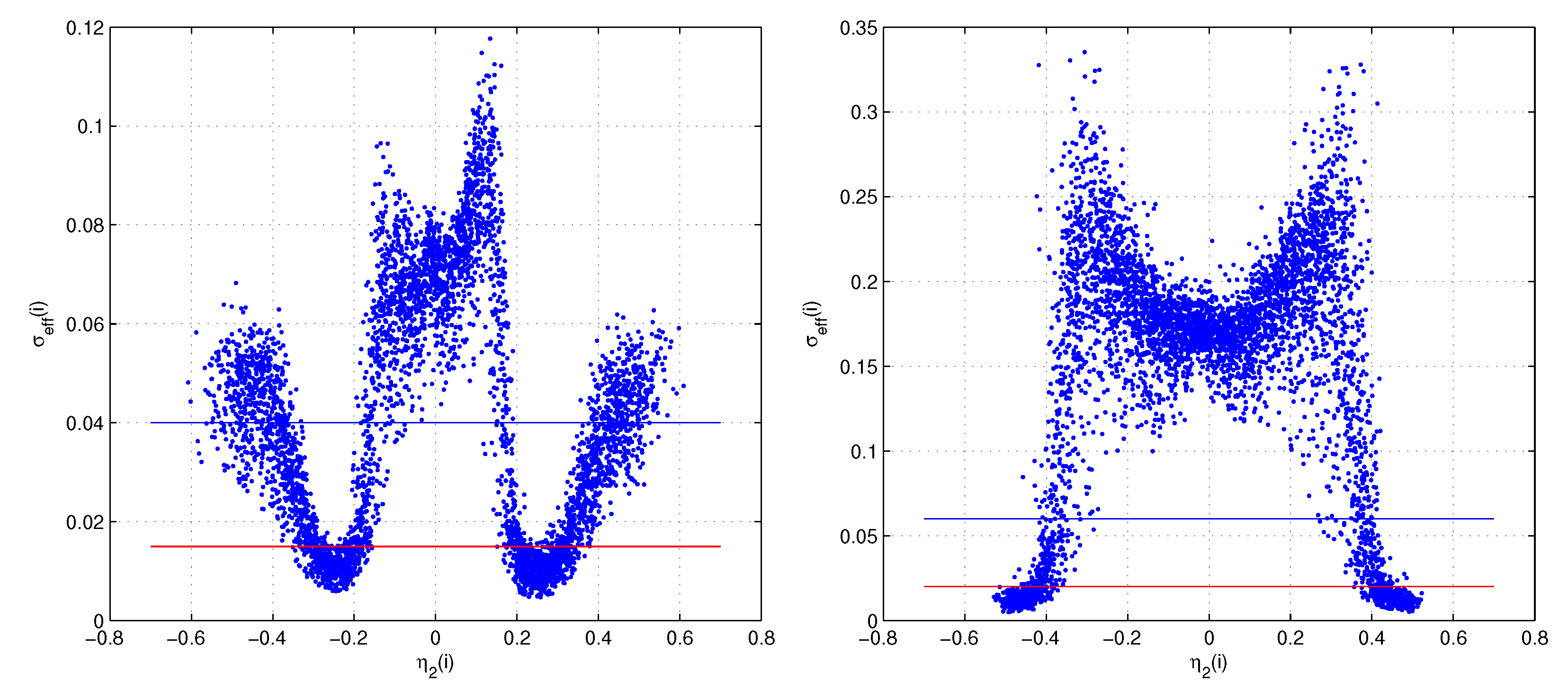
2.3. The Functional Dependence from the Impact Point

For our fitting task, the PDFs with constant a i , the noiseless version of the strip signals, and variable x (the COG 2 noisy values), are irrelevant. We need the PDFs of the impact point ε at constant (noisy) x. It is clear that the mean values { a i } of Equation (4) depend from the impact points and they are related to x by Equation (5). To simplify this dependence we redefine as a i ( ε ) the fraction of signal acquired by each strip as a function of ε , an additional parameter to normalize this fraction must be recovered from data of each hit. The constructions of the functions a i ( ε ) has been illustrated in ref. [9], for orthogonal incidence. Identical expressions will be used here. These new pieces of information, contained in the { a i ( ε ) } , extend the PDF of Equation (3) to be function of the impact point. The PDF can be rewritten as:
P x g 2 ( x , E t , ε ) = F ( a 1 ( ε ) , a 2 ( ε ) , a 3 ( ε ) , E t , σ 1 , σ 2 , σ 3 , x ) x 2 N P ( x ) .
where F ( a 1 ( ε ) , a 2 ( ε ) , a 3 ( ε ) , E t , σ 1 , σ 2 , σ 3 , x ) is the term in square brackets of Equation (3) and N P ( x ) normalizes P x g 2 ( x , E t , ε ) as a function of ε . Equation (6) is the mathematical infrastructure able to connect the points (a)–(c) discussed at the beginning of Section 2. The functions a 1 ( ε ) , a 2 ( ε ) , a 3 ( ε ) are the fractions of signal collected by the strips 1 , 2 , 3 as a function of ε , they are normalized with E t , the total signal of the three strips: the central one with the maximum signal and the two lateral. The extraction of the functions { a i ( ε ) } from real data described in ref. [9] is a delicate operation, but a strict compliance to the described equations produces very reliable results. In any case, slight variations of the { a i ( ε ) } around the best one give almost identical track parameter distributions, thus their selection is very important but less critical than expected. Our function a 2 ( ε ) has a definition similar to the functions called “templates” in ref. [20]. The parameters σ 1 , σ 2 , σ 3 are the standard deviations (Equation (4)) of the three strips considered. Equation (6) can easily handle strips with different σ , but, in the simulations, we will use identical σ s for all the strips of same detector side. To simplify the notations, these parameters will not be reported in the future expressions. A set of PDFs from Equation (6) are illustrated in ref. [9] as ε -functions. It should be evident the enormous number of different PDFs that can be generated by Equation (6), it depends from five parameters and three independent functions (essentially at least hundred free parameters). For the COG 3 case, the equivalent of Equation (6) depends from seven parameters and five independent functions, at large incidence angle this type of PDF is one of the candidates for the fit.

2.4. The η Position Algorithms

Two different position algorithms will be used in the following: the COG 2 algorithm and the η 2 algorithm. The results of the least squares are better with the η 2 positioning algorithm than with the COG 2 . The η 2 -algorithm is built to correct the COG 2 systematic error. Assuming a definite relation of the impact point ε with the COG n , the PDF of the COG n can be defined as the coordinate transformation:
p ( ε ) | d ε d x g n | = Γ n ( x g n ) ,
where Γ n ( x g n ) is the PDF of COG n given by p ( ε ) as PDF of impact points. For uniform distribution of the impact point p ( ε ) = 1 / τ and normalized to one on the strip length τ ( τ = 1 here), the differential equation can be integrated:
ε n ( x g n ) = ε ( x g n 0 ) + x g n 0 x g n Γ n ( y ) d y ,
the positive sign of d ε / d x g n is discussed in refs. [4,8]. With the exact initial constant ε ( x g n 0 ) , the function ε n ( x g n ) is a better estimation of the impact point than the simpler COG n . In the η 2 positioning algorithm, the function ε 2 ( x g 2 ) is given by the experimental COG 2 PDF inserted in Equation (8). The extraction of the initial constant ε ( x g 2 0 ) from the data is discussed in refs. [8,21] and tested in a dedicated test beam [10]. The definition of Equation (7) generalizes the η algorithm of ref. [7] for any COG n . Our η 2 algorithm coincides with that of ref. [7] with ε ( x g 2 0 ) = x g 2 0 = 0 . This condition is true for an exact axial symmetry of the signal distribution and of the strip response function. It is evident that real detectors drastically deviate from this symmetry, and essential corrections must be implemented for ε ( x g 2 0 ) .

2.5. Track Definition

Given the novelty of this approach, our track definition must be very simple. The tracks are circles with a large radius to simulate the high momentum MIPs where the multiple scattering is negligible. The relation of the track parameters to the momenta is p = 0.3 B R (ref. [22]) here p is in GeV / c , B in Tesla and R, the track radius, in meters.
The tracker model is formed by six parallel equidistant ( 89 mm ) detector layers as in the PAMELA tracker. The constant magnetic field is 0.44 T . The simulated tracks are on a plane perpendicular to the the detector layers and to the magnetic field, ( ξ , z ) are the coordinates of the track plane. The center of the tracker is at ξ = 0 , z = 0 , the z axis is parallel to the layer planes and the ξ axis is perpendicular. The tracks are circles with center in ξ = R and z = 0 , and the magnetic field is parallel to the analyzing strips. To simplify the geometry, the overall small rotation of the Lorentz angle ( 0.7 ) is neglected now, but it will be introduced in the following. The simulated hits are generated (ref. [9]) with a uniform random distribution on a strip, they are collected in groups of six to produce the tracks. The exact impact position ε of each hit is subtracted from its reconstructed η 2 ( x g 2 ) position (as defined in refs. [7,8,9]) and it is added the value of the fiducial track for the corresponding detector layer. In this way each group of six hits defines a track with our geometry and the error distribution of η 2 -algorithm. Identically for the COG 2 positioning algorithm. This hit collection simulates a set of tracks populating a large portion of the tracker system with slightly non parallel strips on different layers (as it is always in real detectors). At our high momenta the track bending is very small and the track sagitta is smaller than the strip width. Thus, the bunch of tracks has a transversal section around a strip size, on this width we have to consider the Lorentz angle but its effect is clearly negligible. Our preferred position reconstruction is the η 2 algorithm as in ref. [9] because it gives parameter distributions better than those obtained with the simplest COG 2 positions, but even the results for the COG 2 will be reported in the following.
In the { ξ , z } -plane, the circular tracks are approximated, as usual, with parabolas that are linear in the track parameters:
ξ = R + R 2 z 2 β + γ α z 2 = φ ( z ) ξ n = β n + γ n z α n z 2 = φ n ( z ) .
The first line of Equation (9) is the model track, the second line is the fit result. The circular track is the osculating circle of the parabola φ ( z ) , at our high momenta and tracker size the differences are negligible. The function φ ( z ) has γ = 0 , β = 0 , and 1 / α is proportional to the track momentum. Due to the noise, the reconstructed track has equation φ n ( z ) and the parameters { α n , β n , γ n } , given by the fit, are distributed around the model values. The non gaussian forms of our PDFs oblige the use of the non-linear search of the likelihood maxima, and, as always, the search will be transformed in a minimization. The parameters of the track n are obtained minimizing, with respect to { α n , β n , γ n } , the function L ( α n , β n , γ n ) defined as the negative logarithm of the likelihood with the PDFs of Equation (6):
L ( α n , β n , γ n ) = j = 6 n + 1 6 n + 6 ln [ P x g 2 ( x ( j ) , E t ( j ) , ψ j ( α n , β n , γ n ) ] ψ j ( α n , β n , γ n ) = ε ( j ) φ ( z j ) + φ n ( z j ) .
The parameters x ( j ) , E t ( j ) (introduced in Equation (6)) are respectively: the COG 2 ( j ) position, the sum of signal in the three strips for the hit j of the track n. The term z j is the position of the detector plane j of the nth track. The ε -dependence in the { a i ( ε ) } is modified to ψ j ( α n , β n , γ n ) , to place the impact points on the track. In real data, ε ( j ) φ ( z j ) is absent (and unknown) but the data are supposed to be on a track. We can easily use a non linear form for the function ψ j ( α n , β n , γ n ) , but in this case is of scarce meaning. In more complex cases, non linearities of various origin can be easily implemented, for example analytic expressions of the tracks that exactly account for the magnetic field inhomogeneities.
We will reserve the definition of Maximum Likelihood Evaluation (MLE) for the results of Equation (10). The routine for the MLE is initialized as in ref. [9], the first track parameters are given by a weighted least squares (schematic model) with weights given by an effective variance ( σ e f f ( i ) 2 ) for each hit ( i ) and η 2 ( i ) as hit position. The σ e f f ( i ) 2 is obtained from Equation (6), but, for its form, the variance is an ill defined parameter even in ε . Cuts in the integration limits suppress the tails and give finite results.
σ e f f ( i ) 2 = η 2 ( i ) c t η 2 ( i ) + c t P x g 2 ( x ( i ) , E t ( i ) , ε ) ε η 2 ( i ) 2 d ε .
The parameter c t is selected to reproduce the PDFs P x g 2 ( x ( i ) , E t ( i ) , ε ) with gaussian functions of variance σ e f f ( i ) 2 in the case of excellent hits. For a set of hits (excellent hits), Equation (6) has the form of a narrow high peak and a gaussian, centered in η 2 ( i ) and variance σ e f f ( i ) 2 , can overlap well the P x g 2 ( x ( i ) , E t ( i ) , ε ) around the maximum. We selected a few of them for the tuning of c t . These gaussian approximations look good in linear plots, the logarithmic plots show marked differences even in these happy cases: the tails are non-gaussian. The cuts, so defined, are used for the σ e f f ( i ) extraction for all the other hits, even where P x g 2 ( x ( i ) , E t ( i ) , ε ) is poorly reproduced by a gaussian. We use two sizes of cuts, one for each side of our detector.
The { α n , β n , γ n } given by the schematic model (weighted least squares) are almost always near those given by the minimization of Equation (10), thus accelerating the minimum search to the MATLAB [23] f m i n s e a r c h routine. The closeness of these approximations to the MLE supports the non criticality of the extraction of the functions { a i ( ε ) } . The approximate gaussian distributions are often very different from the hit PDFs but this partial information suffices to produce near optimal results. When the tails of the PDFs are important the MLE gives better results. The strong variations of the set { σ e f f } on the strip are illustrated in Figure 1. The time-consuming extraction of σ e f f ( i ) can be reduced building a look-up table of σ e f f ( η 2 ( x ) , E t ) and calculating σ e f f ( i ) with an interpolation. This use of Equation (11) to get weights to insert in the least squares is directly consistent with ref. [6].
Having to plot the results of four type of reconstructions we will use the following color convention for the lines:
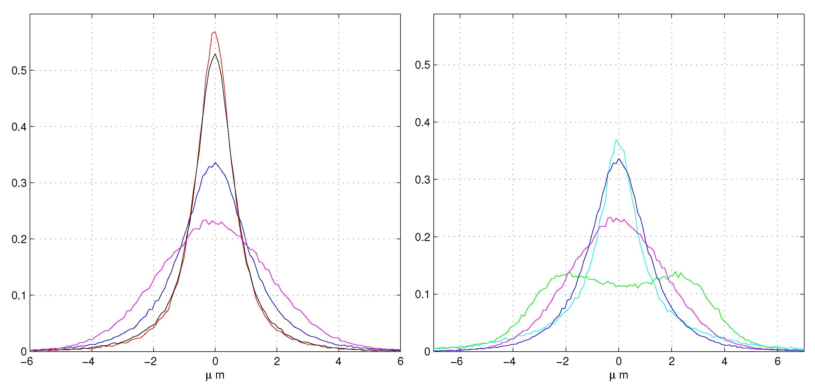
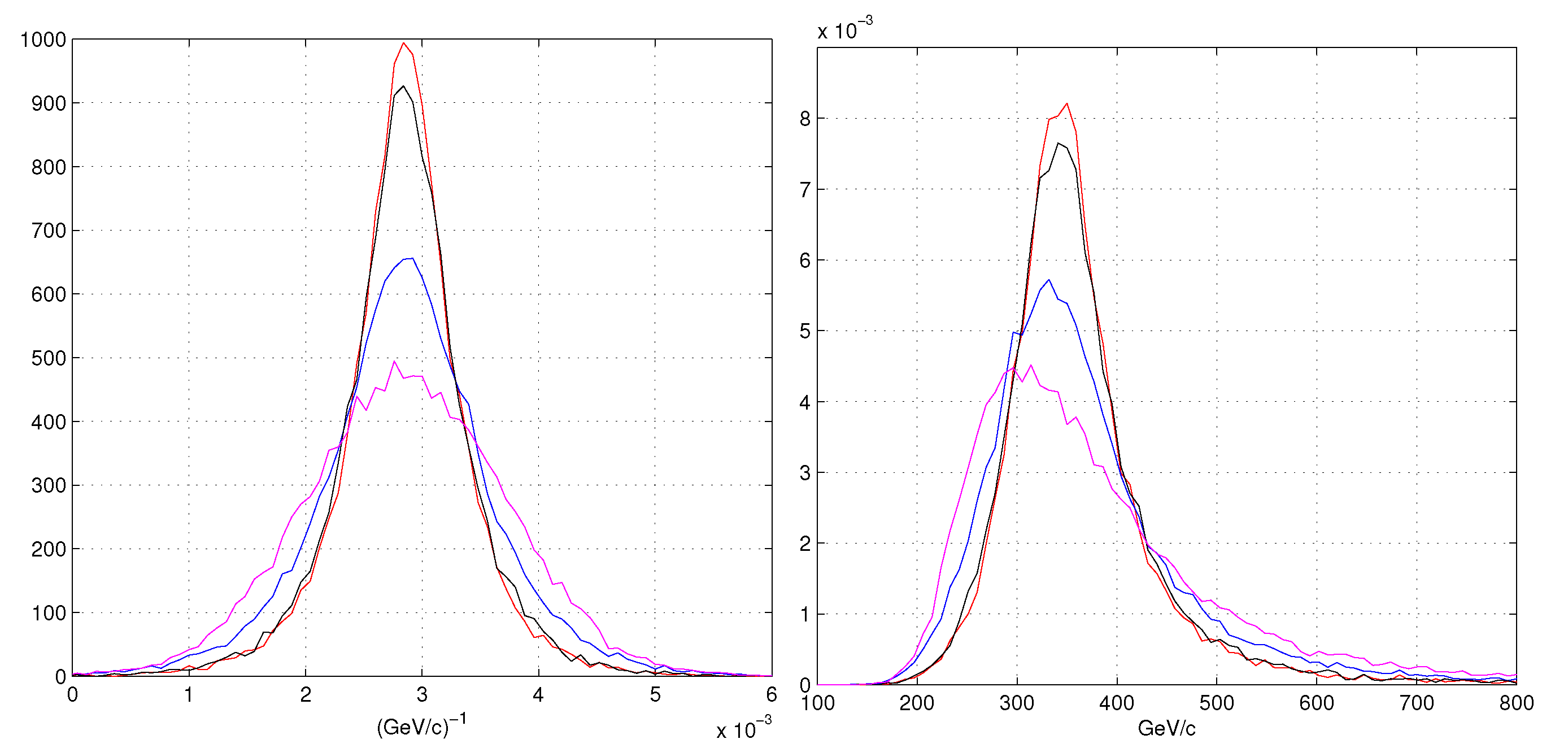
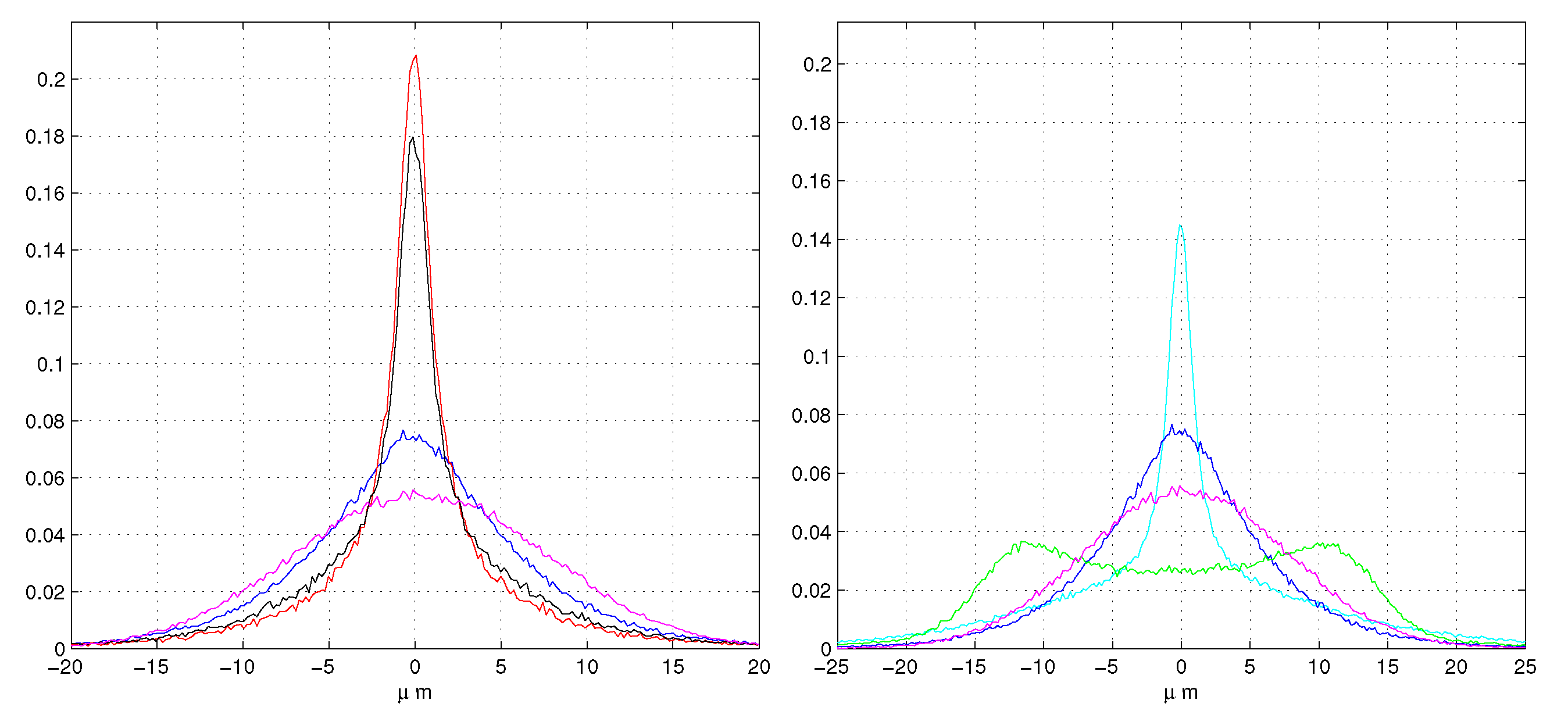
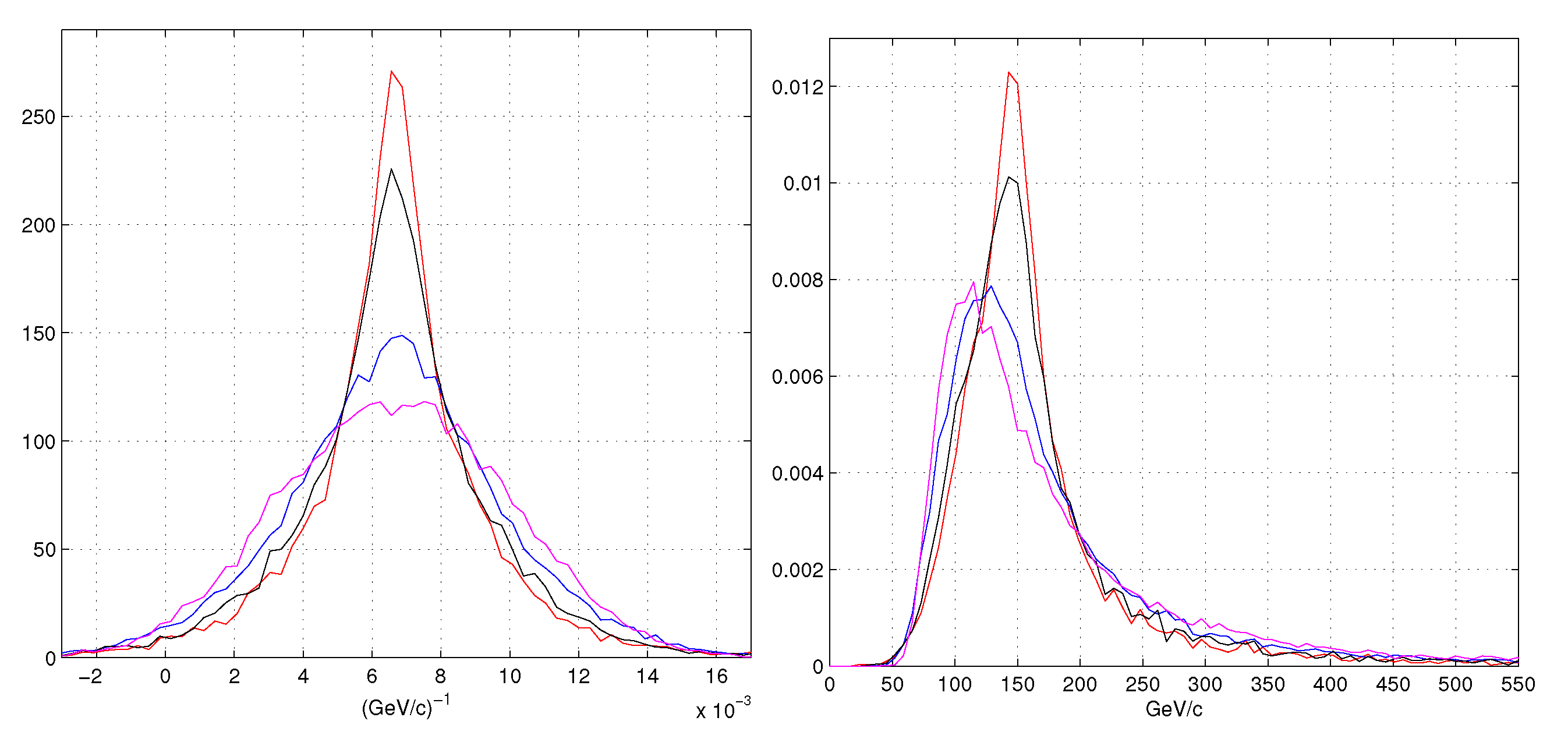
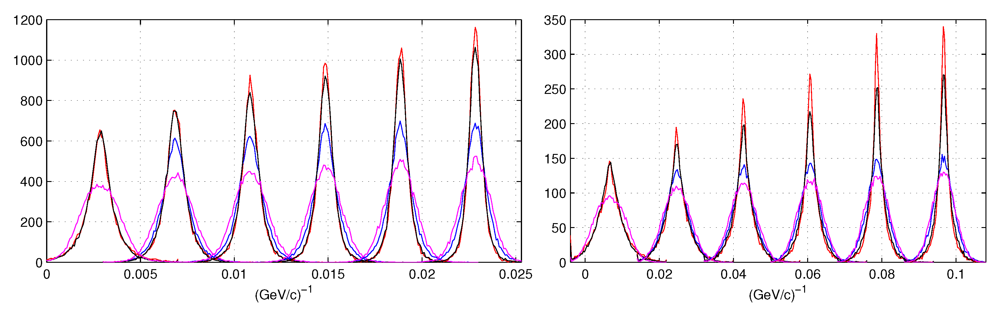
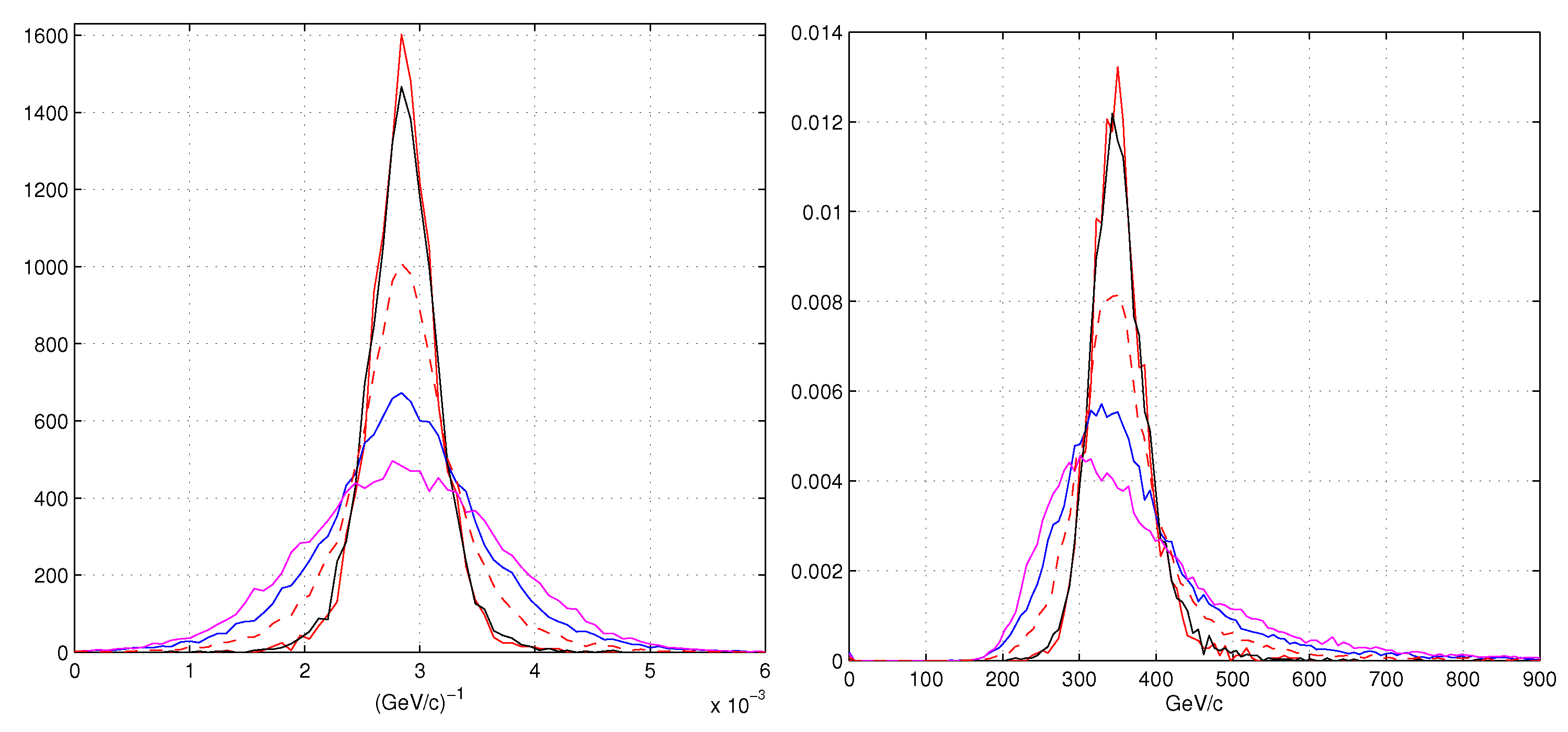
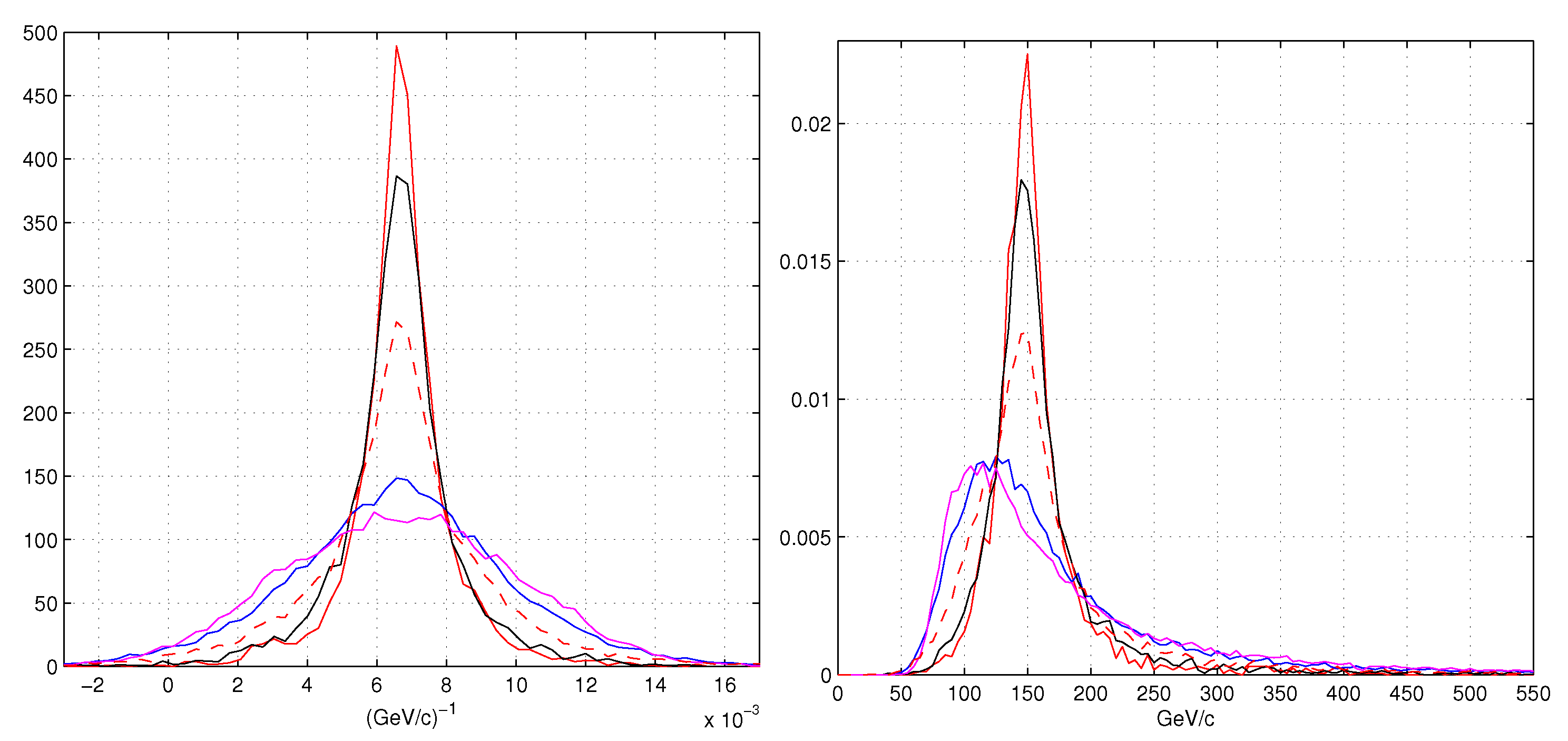
  • red lines: refer to our MLE (Equation (10)),
  • black lines are the weighted least squares with weight 1 / σ e f f ( i ) 2 and η 2 position,
  • blue lines for the least squares with the η 2 position algorithm
  • magenta lines for the least squares with the COG 2 position algorithm.

3. Low Noise, High Resolution, Floating Strip Side

The floating strip side is the best of the two sides of this type of strip detector (strip width 51 μ m, thickness 300 μ m). It is just this side that measures the track bending in the PAMELA magnetic spectrometer. In the test beam [10], the noise PDF of the “average” strips without signals is well reproduced by a gaussian with a standard deviation of 4 ADC counts. The PDF for the sum of three strip signals has its maximum at 142 ADC counts with the most probable signal-to-noise ratio ( S N R ) of 35.5 for a three-strip cluster ( S N R ( n ) = i = 1 3 x i ( n ) / σ i ). The functions a j ( ε ) are those of ref. [9] for this strip type. In the simulations we will use a high momentum of 350 GeV / c . For this momentum and identical geometry, we have a report with some histograms of a CERN test beam of the PAMELA tracker before its installation in the satellite. The tracks were reconstructed with the original η algorithm of ref. [7], the curvature histogram turns out very similar to ours, giving an excellent check of our simulations. In this case, with the orthogonal incidence of the beam, the systematic error of η algorithm of ref. [7] is constant (and small) and has no effect on the curvature reconstruction.
In the left side of Figure 3, the histogram values divided by the number of entries and the step size (frequency polygons called distributions in the following) of the differences of the fitted positions compared to the exact ones (true residuals in the following) are reported. We will use the definition of true residuals (allowed only in simulations) to distinguish from the residuals that generally indicate the differences from the fitted positions with respect to the reconstructed ones. The highest curve is the distribution of the true residuals of our MLE, followed immediately by the true residuals of our schematic model. The true residuals of the least squares with η 2 and COG 2 as hit positions are the lowest two distributions.
Due to the absence of the COG systematic error, the PDFs of the track parameters given by the η 2 algorithm are better than those given by the COG 2 . The right side of Figure 3 illustrates the relations of the true residual PDFs for the least squares with the η 2 and COG 2 as hit positions with their corresponding error PDFs. We see that, contrary to the general expectation, the data redundancy does not improve the position reconstructions for the η 2 algorithm. This result is similar to the use of the least squares with data extracted from a Cauchy distribution: the least squares degrades the original position resolution. Instead, the true residual PDF of COG 2 least squares looks better than the error PDF. The least squares method seems able to round the error distribution, but this effort consumes all its power. In fact, if the statistical noise is suppressed, the COG systematic error does not allow any modification of the true residual PDF. On the contrary, the true residual PDF of the η 2 least squares grows toward a Dirac δ -function in the absence of the statistical noise.
The PDFs of the residuals (as defined above) are not reported. Those for the COG 2 and η 2 are almost identical to the true residual PDFs of Figure 3. The residuals for the MLE and of the schematic model are very different from their true residuals of Figure 3. Narrow and high peaks centered in zero are present in those two distributions. The peak of the schematic model is higher than that of the MLE, and both of them are higher than their maxima of the true residual distributions. Our PDF of Equation (6) and the weights 1 / σ e f f ( i ) 2 distinguish good hits from bad hits and the fit optimization forces the track to pass near to good ones, giving them an high frequency of small residuals. Often the residuals are used as a measure of the detector resolution, it is easy to show the inconsistency of this assumption almost in any case. For example in the right side of Figure 3 the distribution of the true residuals of the COG 2 is very similar to the residual distribution, but it is very different from the COG 2 error distribution. In the following other similar discrepancies will be underlined.
As illustrated in Figure 4, the MLEs give the best results for the momentum reconstruction, and the weighted least squares, are very near to them. The fits of the standard least squares with η 2 or COG 2 positioning algorithms show a drastic decrease in resolution. The use of the simple COG 2 algorithm is the worst one. Often the distributions of the left side of Figure 4 are reported as resolution of the momentum reconstruction, the k-value of ref. [22]. For the η 2 and COG 2 least squares, the plots of the momentum distributions have appreciable shifts of the maxima (most probable value) respect to the fiducial value of 350 GeV / c , the shifts are negligible for the other two fits. These shifts are mathematical consequences of the change of variable from curvature to momentum. For gaussian PDF, the shift of the maximum due to the variable conversion from curvature ( GeV / c 1 ) to momentum ( GeV / c ) is easily calculable, and depends from the variance of the gaussian, increasing the variance the maximum for the momentum PDF moves to lower values.

3.1. Other Track Parameters

The complete track reconstruction must consider even the other two parameters of a track, the β n and γ n . Their fits give very similar distributions to those plotted in ref. [9]. The maxima of the distributions are now a little lower, in particular for the β parameter. This is not unexpected, in ref. [9] we had 3 degrees of freedom for two parameters, here we have 3 degrees of freedom for three parameters, an effective reduction of the redundancy that has a slight effect on the results.

4. High Noise, Low Resolution, Normal Strip Side

The other side of the double sided silicon microstrip detector has very different properties compared to the floating strip side (the junction side). We will not recall the special treatments required to transform this side (the ohmic side) in strip detector and all the other particular setups necessary to its function. From the point of view of their data, this side produces very similar data to a normal strip with a gaussian noise of 8 ADC counts, twice of the other side (most probable signal-to-noise ratio S N R ( n ) = 18.2 ) and a strip width of 63 μ m. The absence of the floating strips gives to the histograms of the COG 2 the normal aspect with a high central density and a drop around x g 2 = 0 . No additional rises around x g 2 = ± 1 / 2 are present, they are typical of the charge spreads given by the floating strips. This absence reduces the efficiency of the positioning algorithms that gain substantially from the charge spread. Now, the functions { a i ( ε ) } of ref. [9] are similar to those of an interval function with a weak rounding to the borders, this rounding is mainly due to the convolution of the strip response with the charge spread produced by the drift in the collecting field. If a residual capacitive coupling is present, it is very small. In any case, it is just this rounding that renders very good the resolution of the hits on the strip borders with a small σ e f f ( i ) (e.g., the points below the lowest horizontal line in Figure 1). Due to the differences with the other side, and to obtain a reasonable momentum distribution we have to implement the simulations with a lower momentum of 150 GeV / c . Operating at higher momentum the curvature distributions has a large part at negative values and the momentum distribution acquires a second maximum at wrong negative momenta.
Figure 5 illustrates the distributions of Figure 3 for this type of detector, that, as discussed above, are much lower than those of Figure 3. As usual, the highest distribution of the true residuals is the MLE, followed by the schematic model with effective σ e f f ( i ) for each hit, the least squares with the η 2 position algorithm, that even here is better than the true residuals of the least squares with COG 2 as position algorithm. As illustrated in the right side of Figure 5, the data redundancy for the least squares with the η 2 -positions is unable to improve its own hit error PDF. The η 2 hit error PDF is drastically better than that of the true residuals for the fit and is the highest distribution of plot. As in Figure 4, the COG 2 position error PDF has two maxima with a separation four times greater than the case of the floating strip side. The COG systematic error is positive for the first half of the strip and negative in the second half and this difference of sign combines to round the two maxima. The fit, based on the COG 2 positions, has a good probability to partially average these sign differences and produce a single wide maximum. The momentum distributions given by the four fits are reported in Figure 6. The results of our MLE and the weighted least squares are drastically better than the standard least squares. Now the shift of the maxima for the momentum distributions of two lowest distributions are more evident than in Figure 4.

5. Discussion

An easy comparison among the different fits is somewhat difficult. Often an effective variance (or a standard deviation) of the PDF is extracted by interpolating a gaussian function on non gaussian distribution to avoid the effects of the tails. However, even the variance itself is not free from arbitrariness as often stated by Gauss in ref. [6], the Gauss preference for the variance is essentially due to its “easier” analytical properties. Similarly the full width at half maximum, as suggested in ref. [22], does not characterize very well non-gaussian distributions. In any case, the differences among the chosen parameters are not of simple interpretation from the physical point of view, and it is precisely the physical point of view that is our essential focus. Here we will use two very “precious” physical resources as measuring tools to establish a comparison: the magnetic field and the signal-to-noise ratio. The simulated magnetic field intensity and the signal-to-noise ratio are increased in the η 2 and COG 2 least squares reconstructions to overlap our best distributions (the red lines). This increase is the relative gain in resolution.

5.1. Increasing the Magnetic Field

With fixed momentum, the magnetic field is increased in the fit for the η 2 least squares. The upper sectors of Figure 7 illustrate these results for the floating strip side and the overlaps with our MLE. The red lines are identical to those of Figure 4, the blue line are the η 2 least squares for tracks with a magnetic field 1.5 times higher. The plots for the COG 2 least squares are not reported to render easily legible the figures, in this case the magnetic field must be increased of factor 1.8 to overlap our red lines. The lowest sectors of Figure 7 report the noisy normal strip side, the red lines are identical to those of Figure 6, the blue lines ( η 2 least squares) overlap the red lines with a magnetic field increased of 1.8 times. Even here, the overlaps with the COG 2 least squares are not reported, but, to obtain reasonable overlaps, the magnetic field must be doubled. Clearly, the increment of the magnetic field produces other slight differences in the tails of the distributions, but the main results are well highlighted.

5.2. Increasing the Signal-to-Noise Ratio

Let us now discuss the effects of the increase of the signal-to-noise ratio. These modifications reproduce in part the results of the magnetic increase, but they are different in other parts. In fact, higher values of the magnetic field do not modify the form of the distributions of the curvature α (with dimension l e g t h 1 ), the curvature distributions translate toward higher values for a reduction of the track radius. The dimensional transformations to ( GeV / c ) 1 and GeV / c have the magnetic field intensity as scaling factor and move the distributions to the forms of Figure 7 even for the COG 2 case. However, as for the α parameters (with dimension l e n g t h 1 ), the distributions of the true residuals of Figure 3 and Figure 5 are not influenced by the increase of the magnetic field, apart small effects on the Lorentz angle.
Keeping the magnetic field to 0.44 T , the increase of the signal-to-noise ratio modifies the distributions of the α parameters and those of the true residuals and can bring them to overlap our red distributions. In our simulations, the increase of the signal-to-noise ratio is accomplished by scaling the amplitude of the random noise, added to the strip signals, and rerunning the least squares fits. The plots of these results for the momentum (in GeV / c ) and curvature (in ( GeV / c ) 1 ) are not reported because they are practically identical to those of Figure 7. For the (low noise) floating strip side, the gaussian strip noise of σ = 4 ADC counts must be reduced to 2.5 ADC counts, increasing the signal-to-noise ratio by a factor 1.6 to a huge most probable value of 56.8 . Now, even the blue line in Figure 3 of the true residuals reaches the red line, but the redundancy continues to be unable to move the true residual distribution beyond that of the new η 2 errors. A special mention must be given to the COG 2 distributions, they remain essentially unchanged in any plot for a (any) reduction of the strip noise. The COG 2 error distribution of Figure 3 (the green line) shows a slight modification becoming less rounded for the hard presence of the systematic error, unaffected by the random noise.
For the noisy normal side of the detector, a reduction to less of one half of the noise (from 8 to 3.6 ADC -counts) is required to reproduce the low parts of Figure 7. With this doubling (2.2) of the signal-to-noise ratio, the blue line (the η 2 best fit) overlaps the red line in Figure 5 increasing the most probable signal-to-noise ratio to 40.5. Similarly to the other side, no noise reduction moves the distributions given by the COG 2 least-squares. As just said above, the absence of response to the noise reduction is due to the COG 2 systematic error of ref. [4]. This fact renders of weak relevance the efforts to improve the signal-to-noise ratio in the detectors if the positioning algorithm remains the uncorrected COG. Unpleasant effects, due to the neglect of the systematic errors, were forecasted long time ago by Gauss [6]. On the other hand, we have also to underline a positive feature of this positioning method. It remains stable to decreases of the signal-to-noise ratio due to ageing or radiation damages, as far as the COG systematic error continues to dominate.
A further point requires an explanation, i.e., the huge difference between the curvature PDF for the η 2 least squares in the low part Figure 7 and the blue line of Figure 4. Now the two detector types have very similar signal-to-noise ratio (3.6 ADC counts in the first and 4 ADC counts in the second), but, to reach the overlap of the two PDFs, another factor of around 2.4 is needed. This factor is too large to be due to the 20% of differences between the sizes of their strips. The main difference must be due to the beneficial charge sharing of the floating strip and the approximation of this architecture to the ideal detector defined in ref. [4]. Thus, detectors without this type of charge sharing are evidently disadvantaged for momentum measurements.

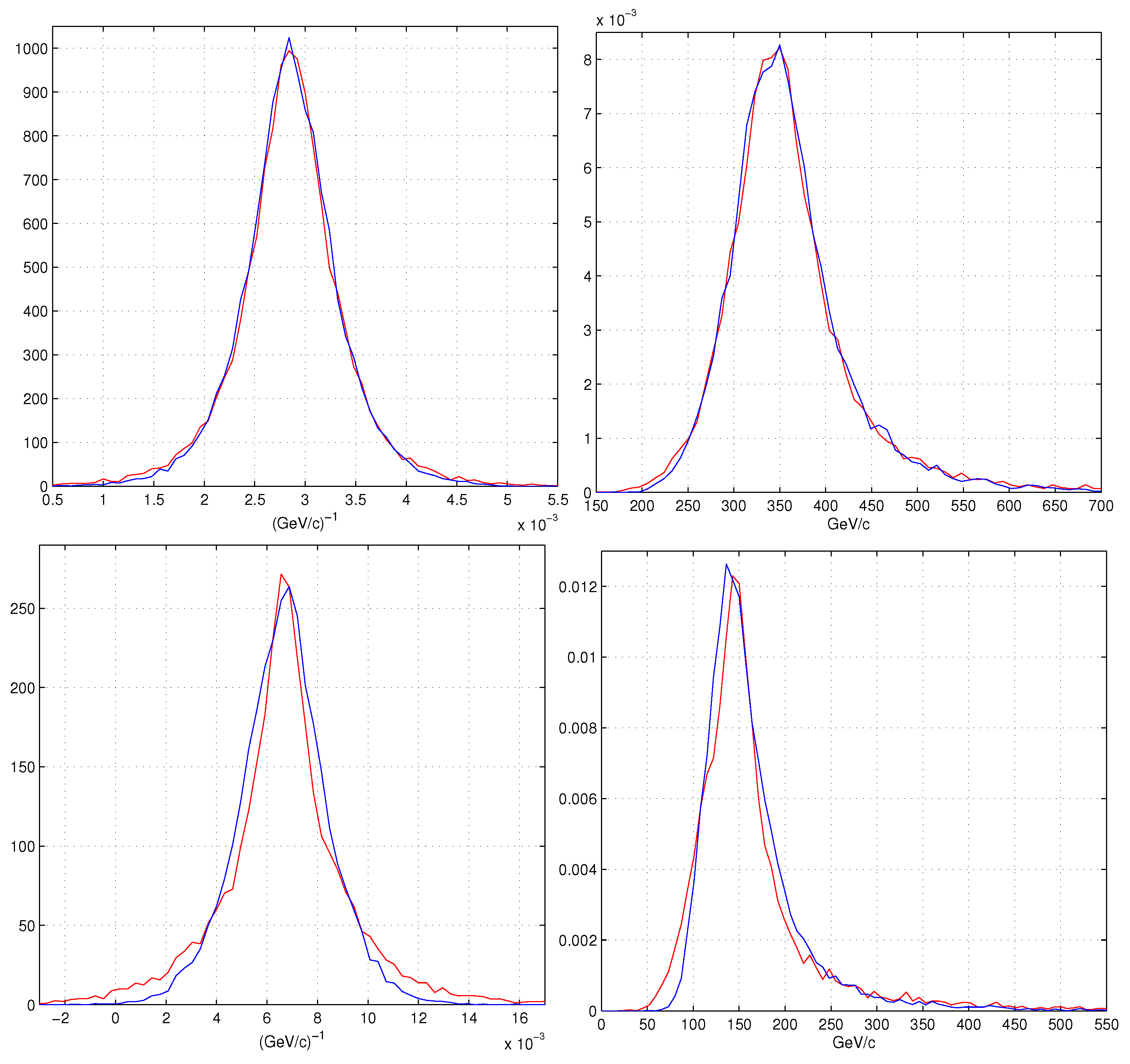
5.3. Momentum Resolution for a Track Selection

Another important result of this new fitting method is the rapid growth of the momentum resolution with the number of detecting layers. The least squares demonstrations assume the identity of the variance of the data to be fitted. This assumption eliminates any statistical difference among the data and the resolution (of a constant) grows with the square root of the number of independent measurements, detecting layers in our case. On the contrary our method distinguishes the hit properties, and the quality of the track reconstruction is controlled by the number of excellent or good hits contained in its path. Thus we can expect that the resolution increases with the number of detecting layers, as the probability of excellent or good hits. To prove this effect we report in Figure 8 the growth in resolution for the curvature PDFs for different numbers of detecting layers.
The PDFs for the six layers set up are those of Figure 4 and Figure 6. A very rapid increase, near to a linear growth with N, is observed for the maxima of the PDFs of our two methods. (For normalized PDFs the maxima are essentially proportional to the inverse of the full-width-at-half-maximum that is often defined as resolution.) The two standard least squares have a typical slow growth of their maxima. To simplify we speak of N even if the curvature grows as a square root of a complicated function of the positions of the detecting layers. In the case of three layers there is an overlap of our two methods with the least squares with the η 2 positioning algorithm. This overlap is due to the absence of any redundancy (zero degrees of freedom) and to the best quality of the η 2 position algorithm with respect to COG 2 . The resolution of the MLE and of the schematic model in the four layers set up results better than the resolution of the six layers set up for the η 2 -least squares. Thus, if this resolution suffices, two detector layers could be eliminated with important saving of weight and energy consumption that are critical parameters for a satellite experiment. However, the four layer resolution is better than the seven and eight layers resolution of the η 2 -algorithm in each of the two detector types. Hence, important reductions of tracker complexity are possible with this new fitting method. Faster growth of resolution with N can be produced with track selections.

5.4. Momentum Resolution for a Track Selection

Up to now, we explored the momentum resolution for a generic track sample without any special attention to the hit quality. All the generated tracks are reconstructed identically. However, our effective variances allow us to select subsets of tracks containing good or excellent hits and to obtain much better momentum resolutions. The numbers of track collected by the running experiments are enormous. The LHC-experiments report track numbers around 10 12 per year, thus subset of data with higher resolution could be relevant for their tasks.
The hit selections are defined in Figure 1, the two horizontal lines isolate the (so called) good hits. The hits below the lowest line are defined excellent hits. It is evident that these are somewhat arbitrary definitions chosen to obtain easy track selections and, with a rough tuning, to have large increases of momentum resolution.
The two last figures illustrate the momentum resolutions of track selections. For the floating strip side, we select tracks with two excellent and three good hits. The 16.1 % of all the tracks has this hit combination, and a very well defined momentum and curvature, drastically better than that without hit selection as illustrated in Figure 9.
We can proceed identically with the noisy normal side. We select tracks with two excellent hits and four other hits of random type, 25 % of tracks has this hit combination. Even in this case the momentum resolution have a great improvement with respect to the case without the hit selection. Figure 10 shows this comparison.

5.5. A “Gift” from Heteroscedasticity

The large variations of the effective variances observed in Figure 1 have effects even in the standard least squares method. The heteroscedasticity couples the track variance to the parameter distributions. Tracks, richer of good or excellent hits (as we defined above), have an higher probability to have lower residual variance. Obviously if the hit reconstruction is free from systematic errors. The η 2 -algorithm has this property. Hence, a track selection with the lowest values of the track residual variance (called χ 2 in ref. [22] ) has the distribution of the reconstructed momenta overlapping our best PDFs of Figure 4 and Figure 5. The price is an efficiency below 25 % but these improvements can be obtained without any modifications of the fitting methods. For the COG 2 hit positions, the χ 2 selection has no “gift” from heteroscedasticity. The COG 2 positioning is dominated by its systematic error that destroys any correlation with good hits.

6. Conclusions

The hit properties of a tracker system are carefully explored for the momentum reconstruction of minimum ionizing particles in a simulated uniform magnetic field of 0.44 T . Other important effects, as δ -rays, multiple scattering (negligible at high momenta), energy loss, etc., are explicitly excluded in the simulations, focusing on the differences among various fitting methods. A simpler and more direct method for the calculation of the probability density functions is illustrated and a useful simplified form, suitable for these applications, is reported. Even if very synthetic, this development completes the other part illustrated in a previous publication and enables the replication of all the published results. The data used for the simulations come from a test beam with double sided detector, which allows the extraction of realistic parameters for the two type of detectors. These parameters are employed to simulate the signals of charged particles in a low magnetic field. The higher noise side has signal properties very similar to single sided detectors of large use in trackers of running experiments. The realistic probability distributions are applied in two forms: complete in the Maximum Likelihood Evaluation or schematic as a weight parameters 1 / σ e f f ( i ) 2 . Each one of these two forms is very effective for the momentum reconstructions compared to the two other type of track fitting i.e., the least squares with η 2 as position algorithm and with the two strip Center of Gravity as position algorithm. To establish a comparison among these fitting methods, the usual method of comparing standard deviations or the full width at half maximum is abandoned. The heavy tails of the distributions give unrealistic contributions to the standard deviation. Instead, two different tracker properties are modified to reach an overlap among the fit outputs: the magnetic field and the signal-to-noise ratio. To reach the overlap of the two standard fits with the best momentum distributions, the magnetic field must grow by a factor 1.5 for the η 2 positioning, and 1.8 for the two strip Center of Gravity in the floating strip side and 1.8 and 2 for the noisy normal side. The increase of signal-to-noise ratio is effective only for the η 2 position algorithm, the overlaps are obtained with factors 1.6 and 2.2 for the two detector sides. Any increase of the signal-to-noise ratio has no effect in the least squares based on two strip Center of Gravity. The intrinsic systematic error of the Center of Gravity as position algorithm survives untouched by any reduction of the detector random noise biasing any position measurement. An evident difference in the resolution of the momentum reconstruction is observed in the noisy normal side with respect to the floating strip side. Even if the noise is reduced to the level of the other side, the momentum resolution remains drastically lower. The effects of the floating strips are very beneficial for momentum resolution. Its approximation of the ideal detector, as defined in a our previous work, attenuates the effects of the heteroscedasticity. The simulations are extended to the study of the effect of the number of detection layers on momentum resolution. It is easy to observe an almost linear increase of resolution of the Maximum Likelihood Evaluation and of the schematic model, as expected, being bound to the linear increase of the average probability for good or excellent hits. Instead, standard fits grow less than the square root of the layer number as for any linear regression model with homoscedasticity. To test the dependence from the hit quality, a rough definition of good and excellent hit is introduced and tracks with a given content of good and excellent hits are selected. These selected tracks show an additional increase of the momentum resolution at the price of an efficiency reduction. It must be reminded that these are simulations and are accompanied with the usual uncertainties of any simulation. Assuming an optimistic view, this increase in resolution can be spent in different ways, either for better results on running experiments or in reducing the complexity of future experiments if the baseline fits (almost always based on the Center of Gravity as position algorithm) are estimated sufficient. Further details about this method will be published elsewhere.

Funding

This research received no external funding.

Conflicts of Interest

The authors declare no conflict of interest.

Abbreviations

The following abbreviations are used in this manuscript:
MIPMinimum Ionizing Particle
PDFProbability Distribution Function
COGCenter of Gravity
COG n Center of Gravity algorithm with n-strips
MLEMaximum Likelihood Evaluation.

References

  1. Berger, N.; Kozlinskiy, A.; Kiehn, M.; Schõning, A. A new three-dimensional fit with multiple scattering. Nucl. Instrum. Methods Phys. Res. A 2017, 844, 135–140. [Google Scholar] [CrossRef]
  2. Blobel, V. A new fast track-fit algorithm based on broken lines. Nucl. Instrum. Methods Phys. Res. A 2006, 566, 14–17. [Google Scholar] [CrossRef] [Green Version]
  3. Karimäki, V. Effective circle fitting for particle trajectories. Nucl. Instrum. Methods Phys. Res. A 1991, 305, 187–191. [Google Scholar] [CrossRef]
  4. Landi, G. Properties of the center of gravity as an algorithm for position measurements. Nucl. Instrum. Methods Phys. Res. A 2002, 485, 698–719. [Google Scholar] [CrossRef]
  5. Landi, G. Properties of the center of gravity as an algorithm for position measurements: Two-dimensional geometry. Nucl. Instrum. Methods Phys. Res. A 2003, 497, 511–534. [Google Scholar] [CrossRef]
  6. Gauss, C.F. Methode de Moindre Carre. Memoires sur la Conbination des Observation; French translation by Bertrand, J.; Revised by the author; Mallet-Bachelier: Paris, France, 1855; Available online: https://books.google.it/books?id=_qzpB3QqQkQC (accessed on 1 September 2018).
  7. Belau, E.; Klanner, R.; Lutz, G.; Neugebauer, E.; Seebrunner, H.J.; Wylie, A. Charge collection in silicon strip detector. Nucl. Instrum. Methods Phys. Res. A 1983, 214, 253–260. [Google Scholar] [CrossRef]
  8. Landi, G. Problems of position reconstruction in silicon microstrip detectors. Nucl. Instrum. Methods Phys. Res. A 2005, 554, 226–246. [Google Scholar] [CrossRef]
  9. Landi, G.; Landi, G.E. Improvement of track reconstruction with well tuned probability distributions. JINST 2014, 9, P10006. [Google Scholar] [CrossRef]
  10. Adriani, O.; Bongi, M.; Bonechi, L.; Bottai, S.; Castellini, G.; Fedele, D.; Grandi, M.; Papini, P.; Vannuccini, E.; Taddei, E.; et al. In-flight performance of the PAMELA magnetic spectrometer. In Proceedings of the 16th International Workshop on Vertex Detectors, Lake Placid, NY, USA, 23–28 September 2007. [Google Scholar]
  11. Batignani, G.; Bosi, F.; Bosisio, L.; Conti, A.; Focardi, E.; Forti, F.; Giorgi, M.A.; Parrini, G.; Scarlini, E.; Tempesta, P.; et al. Double sided read out silicon strip detectors for the ALEPH minivertex. Nucl. Instrum. Methods Phys. Res. A 1989, 277, 147–153. [Google Scholar] [CrossRef]
  12. Adriani, O.; Alcaraz, J.; Ahlen, S.; Ambrosi, G.; Basçhirotto, A.; Battiston, R.; Bay, A.; Bencze, G.; Bertucci, B.; Biasini, M.; et al. The New double sided silicon microvertex detector for the L3 experiment. Nucl. Instrum. Methods Phys. Res. A 1994, 348, 431–435. [Google Scholar] [CrossRef]
  13. Picozza, P.; Galper, A.M.; Castellini, G.; Adriani, O.; Altamura, F.; Ambriola, M.; Barbarino, G.C.; Basili, A.; Bazilevskaja, G.A.; Bencardino, R.; et al. PAMELA-A Payload for Matter Antmatter Exploration and Light-nuclei Astrophysics. Astropart. Phys. 2007, 27, 296–315. [Google Scholar] [CrossRef] [Green Version]
  14. Frühwirth, R. Track fitting with non-Gaussian noise. Comput. Phys. Commun. 1997, 100, 1–16. [Google Scholar] [CrossRef]
  15. Frühwirth, R.; Speer, T. A Gaussian-sum filter for vertex reconstruction. Nucl. Instrum. Methods Phys. Res. A 2004, 534, 217–221. [Google Scholar] [CrossRef] [Green Version]
  16. ALICE Collaboration. The ALICE experiment at the CERN LHC. JINST 2008, 3, S08002. [Google Scholar] [CrossRef]
  17. ATLAS Collaboration. The ATLAS experiment at the CERN Large Hadron Collider. JINST 2008, 3, S08003. [Google Scholar] [CrossRef]
  18. CMS Collaboration. The CMS experiment at the CERN Large Hadron Collider. JINST 2008, 3, S08004. [Google Scholar] [CrossRef]
  19. CMS Collaboration. The performance of the CMS muon detector in proton-proton collision at s = 7 TeV at the LHC. JINST 2013, 8, P11002. [Google Scholar] [CrossRef]
  20. The CMS Collaboration. Description and performance of track and primary-vertex reconstruction with the CMS tracker. JINST 2014, 9, P10009. [Google Scholar] [CrossRef]
  21. Landi, G.; Landi, G.E. Asymmetries in Silicon Microstrip Response Function and Lorentz Angle. arXiv, 2014; arXiv:1403.4273. [Google Scholar]
  22. Olive, K.A.; Agashe, K.; Amsler, C.; Antonelli, M.; Arguin, J.-F.; Asner, D.M.; Baer, H.; Band, H.R.; Barnett, R.M.; Basaglia, T.; et al. Particle Data Group. Chin. Phys. C 2014, 38, 090001. [Google Scholar] [CrossRef]
  23. MATLAB 8, The MathWorks Inc.: Natick, MA, USA.
Figure 1. (Left figure) scatter-plot of the σ e f f ( i ) for the floating strip side as a function of the η 2 positions. (Right figure) scatter-plot of the σ e f f ( i ) for the normal noisy side (with evident lower resolution). The horizontal lines will be illustrated in Section 5.4.
Instruments 02 00022 g001
Figure 2. (Left plot) blue dots: distribution of COG 2 for the floating strip side, continuous line η 2 algorithm. (Right plot) red line, PDF of eq.2.5 along the black line of the left-side figure. Blue line: the simulated COG 2 PDF with Landau fluctuations along the track (0.2 Mega-samples).
Instruments 02 00022 g002
Figure 3. (Left plot) true residuals of the reconstructed tracks. MLE (red), schematic model σ e f f ( i ) (black), hit position η 2 (blue), hit position COG 2 (magenta). (Right plot) position errors of the η 2 (cyan) true residuals for the hit position η 2 (blue), true residual for hit position COG 2 (magenta), and errors of the COG 2 (green).
Instruments 02 00022 g003
Figure 4. (Left plot) distributions of the curvature in ( GeV / c ) 1 (the α parameters) MLE (red), schematic model σ e f f ( i ) (black), hit position η 2 (blue), hit position COG 2 (magenta). (Right plot) reconstructed momentum distributions. Color code as in the left plot.
Instruments 02 00022 g004
Figure 5. The noisy normal strip side. (Left plot) True residuals of the reconstructed tracks. MLE (red), schematic model σ e f f ( i ) (black), hit position η 2 (blue), hit position COG 2 (magenta). (Right plot) position errors of the η 2 (cyan) true residuals for the hit position η 2 (blue), true residual for hit position COG 2 (magenta), and errors of the COG 2 (green).
Instruments 02 00022 g005
Figure 6. (Left plot) distributions of the curvature in ( GeV / c ) 1 (the α parameters) MLE (red), schematic model σ e f f ( i ) (black), hit position η 2 (blue), hit position COG 2 (magenta). (Right plot) distributions of the reconstructed momenta.
Instruments 02 00022 g006
Figure 7. (Top plots) floating strip side, Curvature in ( GeV / c ) 1 and momentum distributions for our MLE (red lines) and η 2 least squares (blue lines) with a magnetic field increased by a factor 1.5. (Bottom plots) noisy normal strip side, here the η 2 least square has a magnetic field 1.8 times greater than the MLE.
Instruments 02 00022 g007
Figure 8. Left plot. Distributions of the curvature in ( GeV / c ) 1 (the α parameters) for the low noise detector and increasing the number of detecting layers. The starting one has three layers (zero degree of freedom), the second has four layers (1 degree of freedom) and is shifted by a fixed step to avoid the overlap with the first one. Similarly for the other that have five, six, seven and eight detecting layers. The right plot is similar for the higher noise side.
Instruments 02 00022 g008
Figure 9. Left plot. Distributions of the curvature in ( GeV / c ) 1 (the α parameters) for the low noise detector for a selection of two excellent and three good hits. The two highest distributions are the MLE and schematic model. The two lowest distributions and the dashed one are those of Figure 3. To the right the momentum distributions.
Instruments 02 00022 g009
Figure 10. Left plot. Distributions of the curvature in ( GeV / c ) 1 (the α parameters) for the high noise detector for a selection of two excellent hits. The two highest distributions are the MLE and schematic model. The two lowest distributions and the dashed one are those of Figure 3. To the right the momentum distributions.
Instruments 02 00022 g010

