


Fully Microscopic Treatment of Magnetic Field Using Bogoliubov–De Gennes Approach

 , , , , and
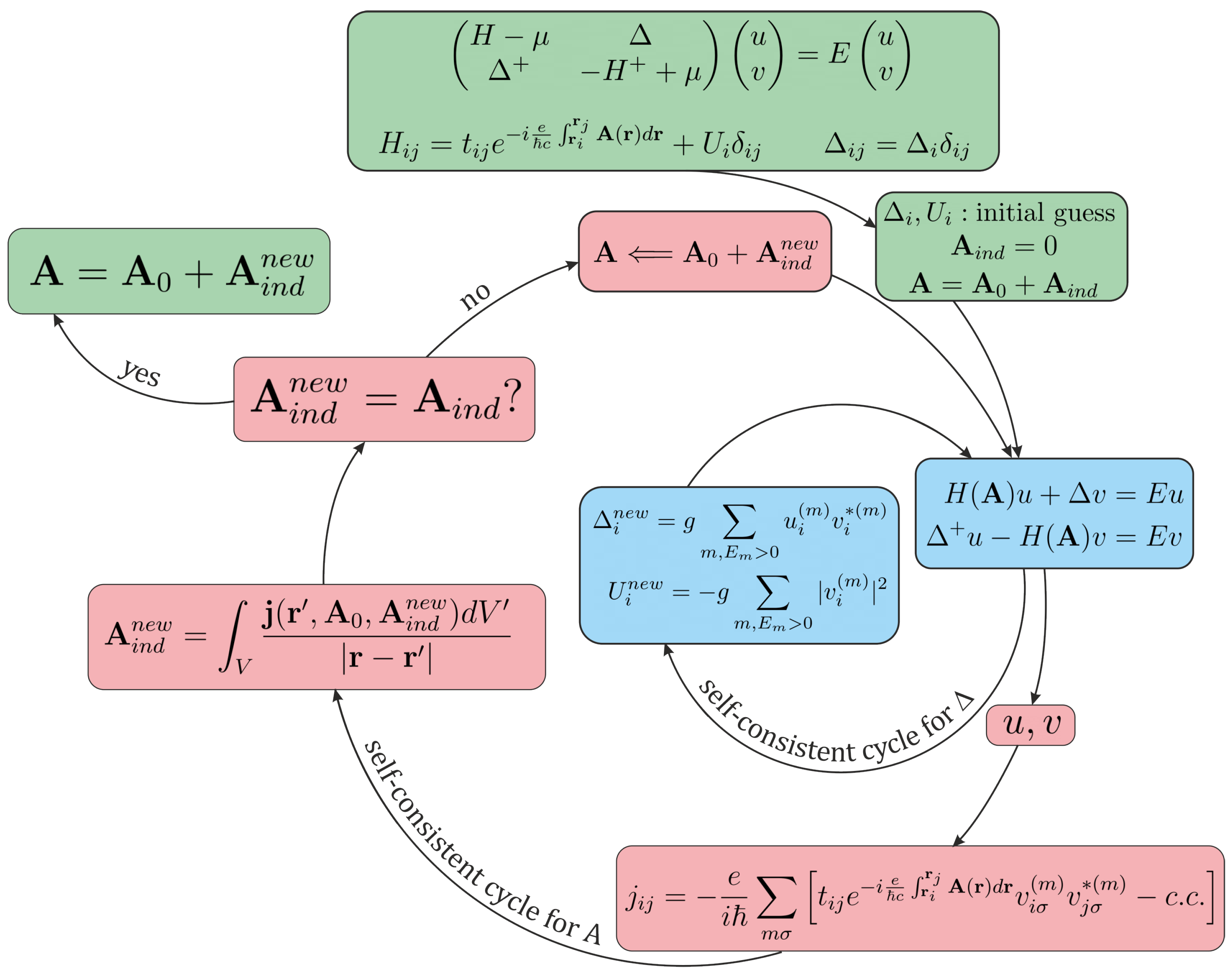
Abstract
1. Introduction
2. Method
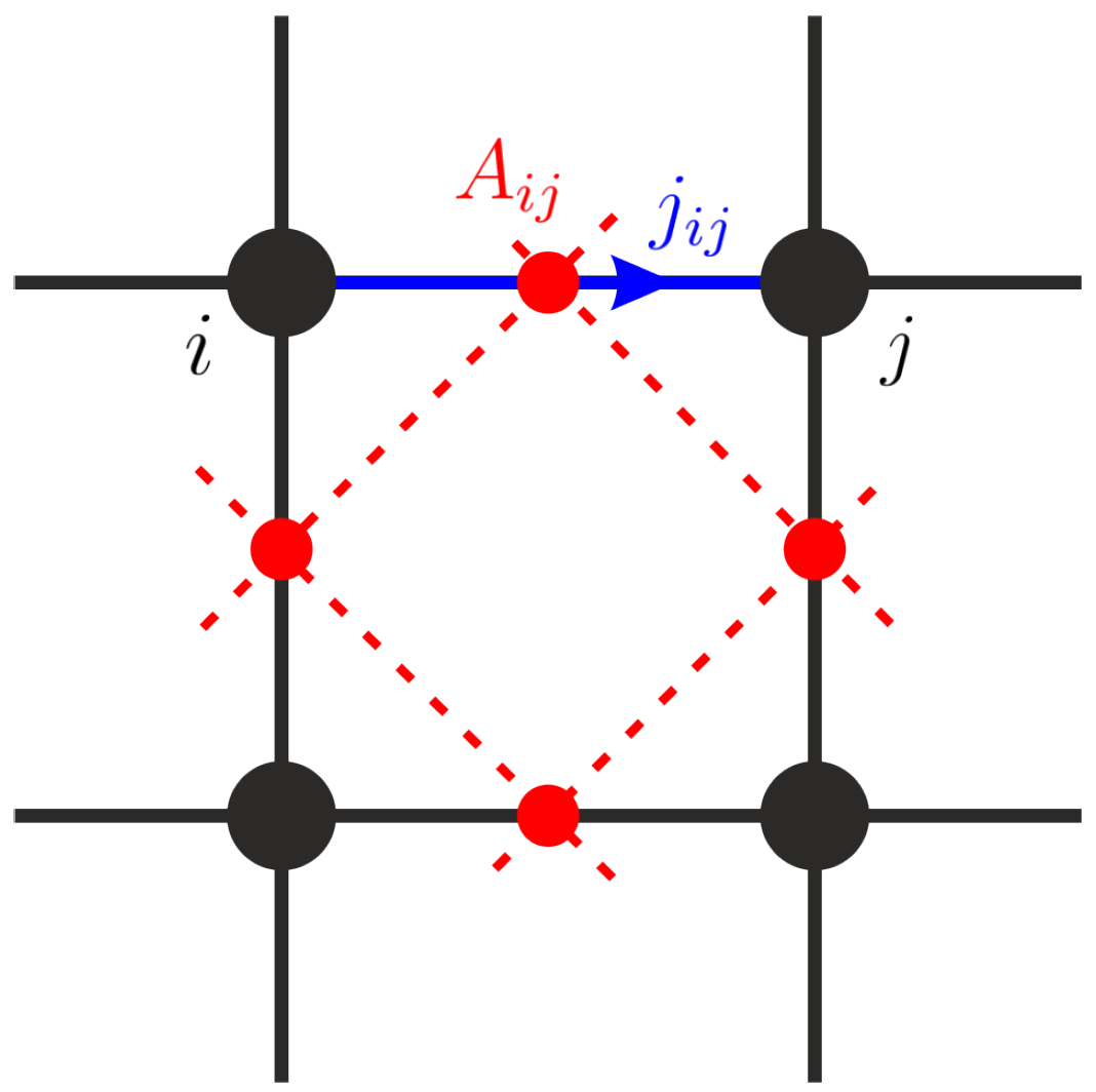
2.1. Formalism
2.2. Inner Convergence Cycle—ICC
2.3. Outer Convergence Cycle—OCC
3. Illustrative Examples
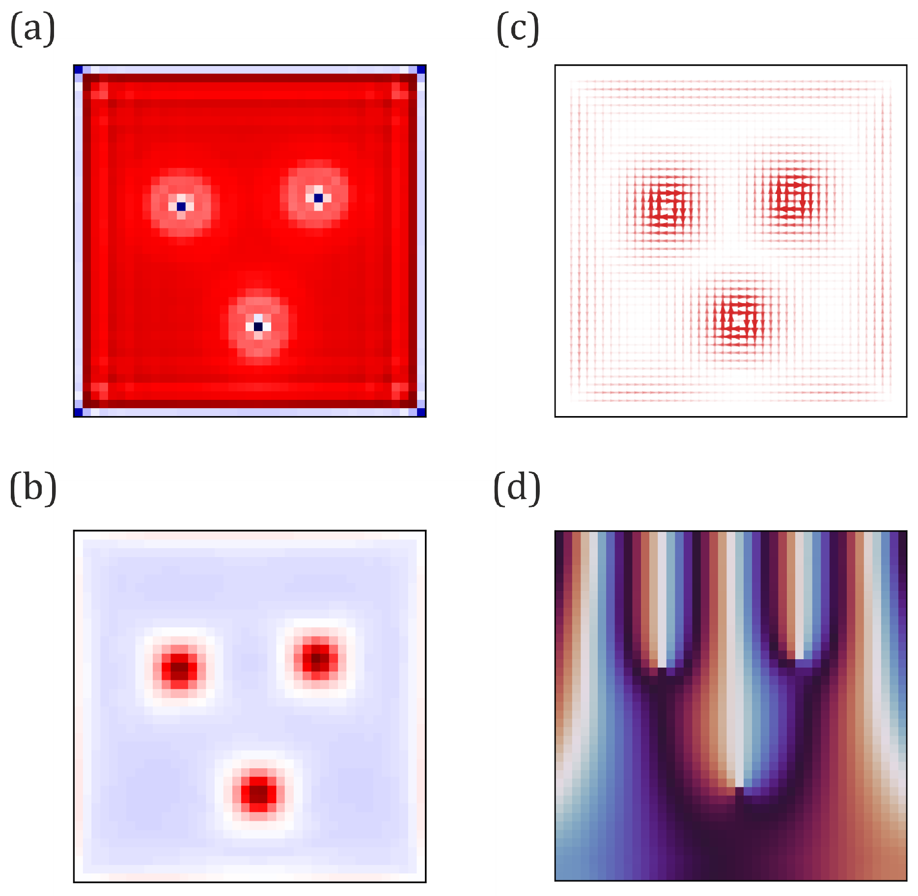
3.1. Abrikosov Lattice
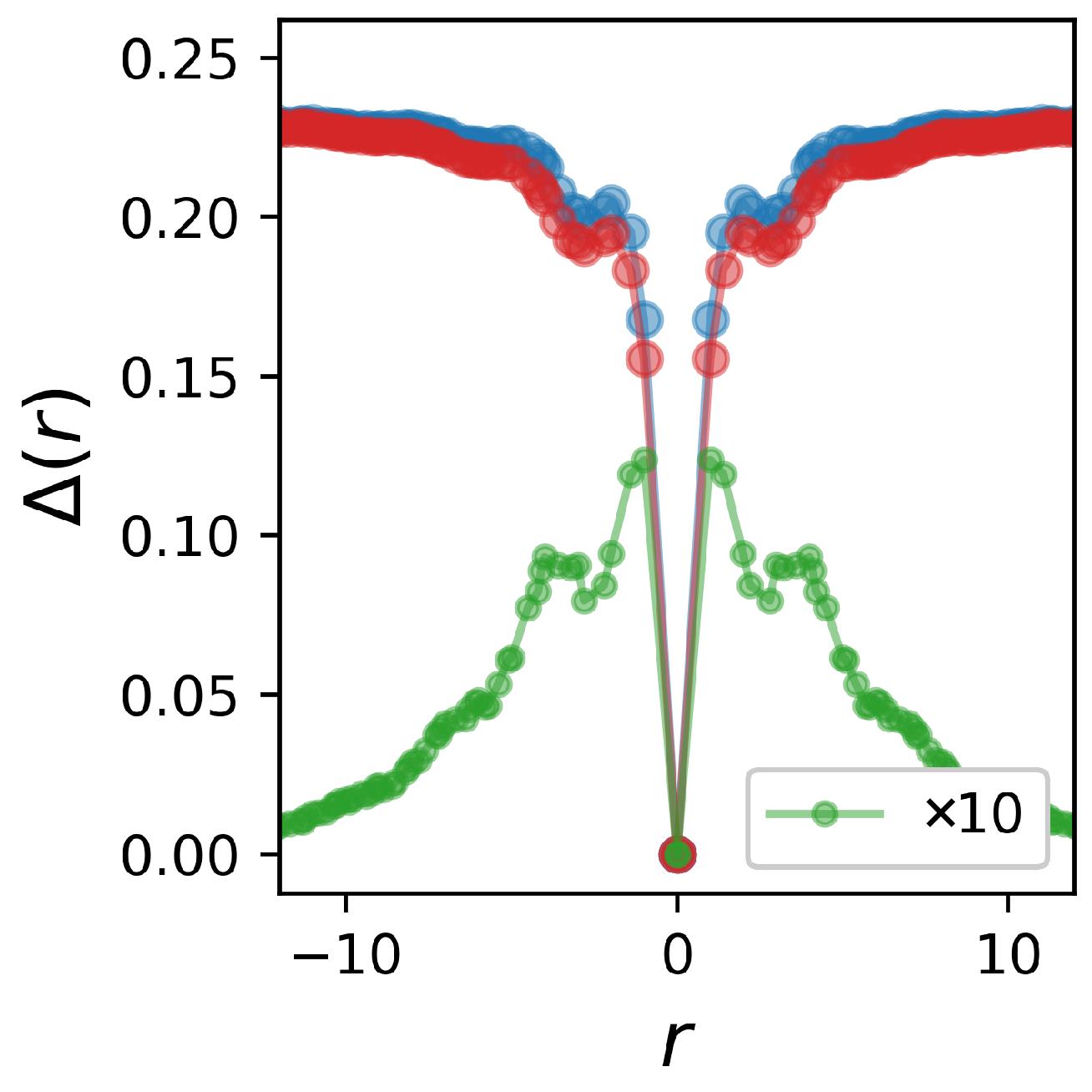
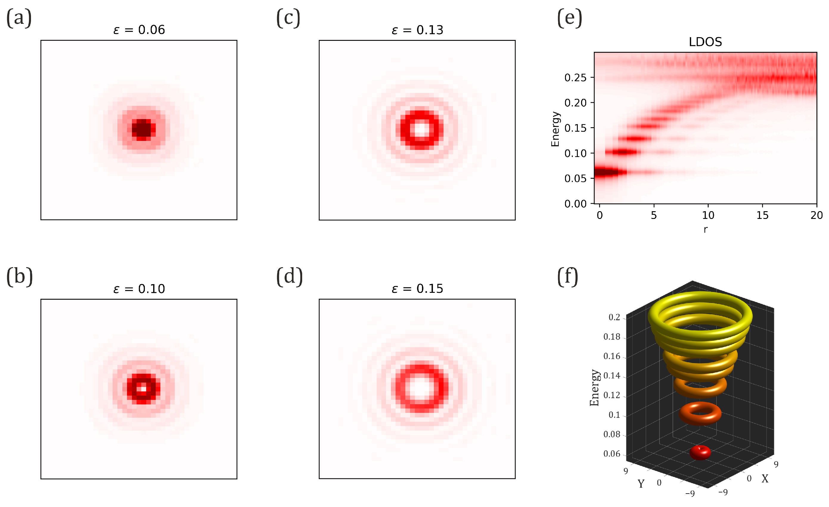
3.2. Vortex Core States
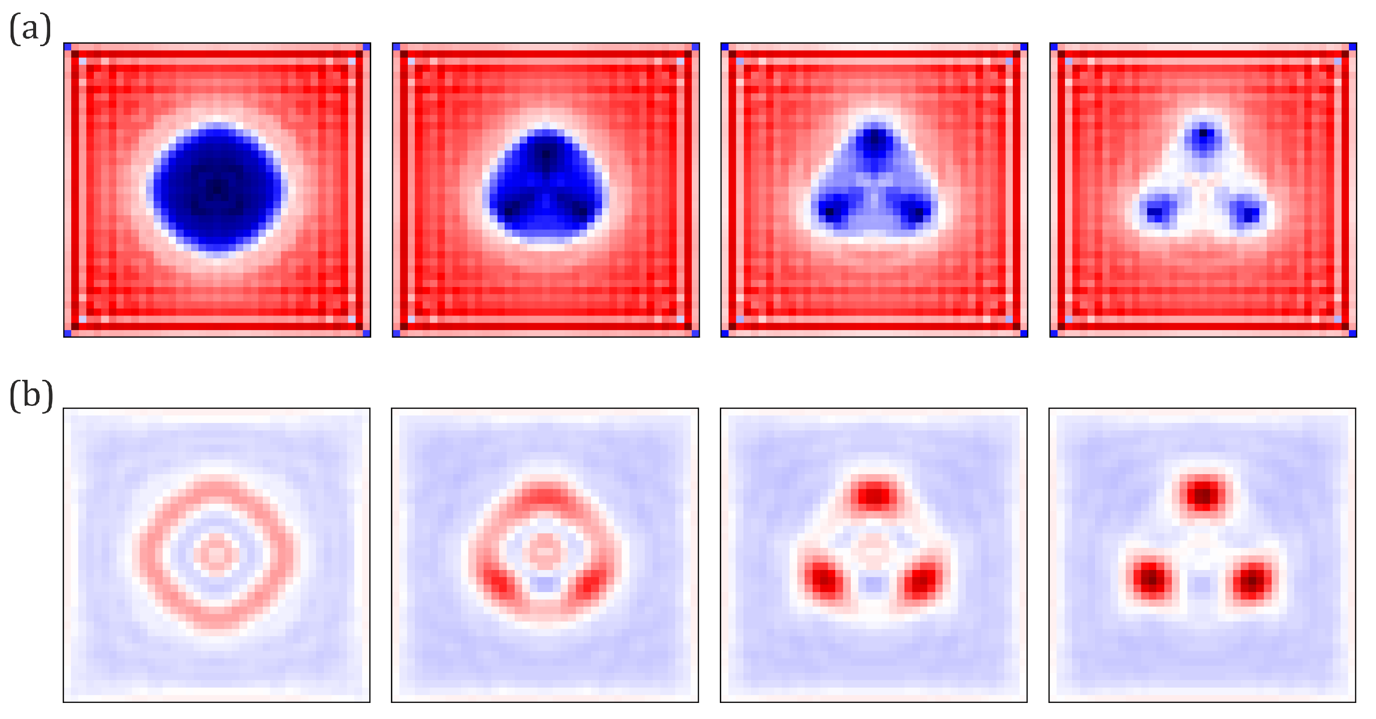
3.3. Intermediate Mixed State
4. Discussion
Author Contributions
Funding
Data Availability Statement
Conflicts of Interest
References
- Abrikosov, A.A. Nobel Lecture: Type-II superconductors and the vortex lattice. Rev. Mod. Phys. 2004, 76, 975–979. [Google Scholar] [CrossRef]
- Caroli, C.; Gennes, P.D.; Matricon, J. Bound Fermion states on a vortex line in a type II superconductor. Phys. Lett. 1964, 9, 307–309. [Google Scholar] [CrossRef]
- Bardeen, J.; Kümmel, R.; Jacobs, A.E.; Tewordt, L. Structure of Vortex Lines in Pure Superconductors. Phys. Rev. 1969, 187, 556–569. [Google Scholar] [CrossRef]
- Shore, J.D.; Huang, M.; Dorsey, A.T.; Sethna, J.P. Density of states in a vortex core and the zero-bias tunneling peak. Phys. Rev. Lett. 1989, 62, 3089–3092. [Google Scholar] [CrossRef] [PubMed]
- Gygi, F.; Schluter, M. Electronic tunneling into an isolated vortex in a clean type-II superconductor. Phys. Rev. B 1990, 41, 822–825. [Google Scholar] [CrossRef]
- Gygi, F.; Schluter, M. Angular band structure of a vortex line in a type-II superconductor. Phys. Rev. Lett. 1990, 65, 1820–1823. [Google Scholar] [CrossRef] [PubMed]
- Gygi, F.; Schlüter, M. Self-consistent electronic structure of a vortex line in a type-II superconductor. Phys. Rev. B 1991, 43, 7609–7621. [Google Scholar] [CrossRef]
- Kramer, L.; Pesch, W. Core structure and low-energy spectrum of isolated vortex lines in clean superconductors atT ≪T c. Z. Phys. 1974, 269, 59–64. [Google Scholar] [CrossRef]
- Hayashi, N.; Isoshima, T.; Ichioka, M.; Machida, K. Low-Lying Quasiparticle Excitations around a Vortex Core in Quantum Limit. Phys. Rev. Lett. 1998, 80, 2921–2924. [Google Scholar] [CrossRef]
- Shanenko, A.A.; Croitoru, M.D.; Peeters, F.M. Magnetic-field induced quantum-size cascades in superconducting nanowires. Phys. Rev. B 2008, 78, 024505. [Google Scholar] [CrossRef]
- Abrikosov, A. The magnetic properties of superconducting alloys. J. Phys. Chem. Solids 1957, 2, 199–208. [Google Scholar] [CrossRef]
- Vagov, A.; Wolf, S.; Croitoru, M.D.; Shanenko, A.A. Universal flux patterns and their interchange in superconductors between types I and II. Commun. Phys. 2020, 3, 58. [Google Scholar] [CrossRef]
- Han, Q. A method of studying the Bogoliubov–de Gennes equations for the superconducting vortex lattice state. J. Phys. Condens. Matter 2009, 22, 035702. [Google Scholar] [CrossRef] [PubMed]
- Berdiyorov, G.R.; Hernandez, A.D.; Peeters, F.M. Confinement Effects on Intermediate-State Flux Patterns in Mesoscopic Type-I Superconductors. Phys. Rev. Lett. 2009, 103, 267002. [Google Scholar] [CrossRef] [PubMed]
- Datta, A.; Banerjee, A.; Trivedi, N.; Ghosal, A. New paradigm for a disordered superconductor in a magnetic field. arXiv 2021, arXiv:2101.00220. [Google Scholar] [CrossRef]
- Fan, B.; García-García, A.M. Exploring the vortex phase diagram of Bogoliubov-de Gennes disordered superconductors. arXiv 2022, arXiv:2205.12347. [Google Scholar] [CrossRef]
- de Braganca, R.H.; Croitoru, M.D.; Shanenko, A.A.; Aguiar, J.A. Effect of Material-Dependent Boundaries on the Interference Induced Enhancement of the Surface Superconductivity Temperature. J. Phys. Chem. Lett. 2023, 14, 5657–5664. [Google Scholar] [CrossRef]
- Ghosal, A.; Randeria, M.; Trivedi, N. Inhomogeneous pairing in highly disordered s-wave superconductors. Phys. Rev. B 2001, 65, 014501. [Google Scholar] [CrossRef]
- Bouadim, K.; Loh, Y.L.; Randeria, M.; Trivedi, N. Single- and two-particle energy gaps across the disorder-driven superconductor–insulator transition. Nat. Phys. 2011, 7, 884–889. [Google Scholar] [CrossRef]
- Gastiasoro, M.N.; Andersen, B.M. Enhancing superconductivity by disorder. Phys. Rev. B 2018, 98, 184510. [Google Scholar] [CrossRef]
- Neverov, V.D.; Lukyanov, A.E.; Krasavin, A.V.; Vagov, A.; Croitoru, M.D. Correlated disorder as a way towards robust superconductivity. Commun. Phys. 2022, 5, 177. [Google Scholar] [CrossRef]
- Liesen, J.; Strakos, Z. Krylov Subspace Methods: Principles and Analysis; Oxford University Press: Oxford, UK, 2002. [Google Scholar]
- Maggio-Aprile, I.; Renner, C.; Erb, A.; Walker, E.; Fischer, O. Direct Vortex Lattice Imaging and Tunneling Spectroscopy of Flux Lines on YBa2Cu3O7-δ. Phys. Rev. Lett. 1995, 75, 2754–2757. [Google Scholar] [CrossRef] [PubMed]
- Vagov, A.; Shanenko, A.A.; Milošević, M.V.; Axt, V.M.; Vinokur, V.M.; Aguiar, J.A.; Peeters, F.M. Superconductivity between standard types: Multiband versus single-band materials. Phys. Rev. B 2016, 93, 174503. [Google Scholar] [CrossRef]
- Córdoba-Camacho, W.Y.; da Silva, R.M.; Vagov, A.; Shanenko, A.A.; Aguiar, J.A. Between types I and II: Intertype flux exotic states in thin superconductors. Phys. Rev. B 2016, 94, 054511. [Google Scholar] [CrossRef]
- Volkov, A.F.; Kogan, S.M. Collisionless relaxation of the energy gap in superconductors. Sov. J. Exp. Theor. Phys. 1974, 38, 1018–1021. [Google Scholar]
- Hannibal, S.; Kettmann, P.; Croitoru, M.D.; Axt, V.M.; Kuhn, T. Persistent oscillations of the order parameter and interaction quench phase diagram for a confined Bardeen-Cooper-Schrieffer Fermi gas. Phys. Rev. A 2018, 98, 053605. [Google Scholar] [CrossRef]
- Berdiyorov, G.R.; Hernández-Nieves, A.D.; Milošević, M.V.; Peeters, F.M.; Domínguez, D. Flux-quantum-discretized dynamics of magnetic flux entry, exit, and annihilation in current-driven mesoscopic type-I superconductors. Phys. Rev. B 2012, 85, 092502. [Google Scholar] [CrossRef]


Disclaimer/Publisher’s Note: The statements, opinions and data contained in all publications are solely those of the individual author(s) and contributor(s) and not of MDPI and/or the editor(s). MDPI and/or the editor(s) disclaim responsibility for any injury to people or property resulting from any ideas, methods, instructions or products referred to in the content. |
© 2024 by the authors. Licensee MDPI, Basel, Switzerland. This article is an open access article distributed under the terms and conditions of the Creative Commons Attribution (CC BY) license (https://creativecommons.org/licenses/by/4.0/).
Share and Cite
Neverov, V.D.; Kalashnikov, A.; Lukyanov, A.E.; Krasavin, A.V.; Croitoru, M.D.; Vagov, A. Fully Microscopic Treatment of Magnetic Field Using Bogoliubov–De Gennes Approach. Condens. Matter 2024, 9, 8. https://doi.org/10.3390/condmat9010008
Neverov VD, Kalashnikov A, Lukyanov AE, Krasavin AV, Croitoru MD, Vagov A. Fully Microscopic Treatment of Magnetic Field Using Bogoliubov–De Gennes Approach. Condensed Matter. 2024; 9(1):8. https://doi.org/10.3390/condmat9010008
Chicago/Turabian StyleNeverov, Vyacheslav D., Alexander Kalashnikov, Alexander E. Lukyanov, Andrey V. Krasavin, Mihail D. Croitoru, and Alexei Vagov. 2024. "Fully Microscopic Treatment of Magnetic Field Using Bogoliubov–De Gennes Approach" Condensed Matter 9, no. 1: 8. https://doi.org/10.3390/condmat9010008
APA StyleNeverov, V. D., Kalashnikov, A., Lukyanov, A. E., Krasavin, A. V., Croitoru, M. D., & Vagov, A. (2024). Fully Microscopic Treatment of Magnetic Field Using Bogoliubov–De Gennes Approach. Condensed Matter, 9(1), 8. https://doi.org/10.3390/condmat9010008