1. Introduction
There is a fundamental distinction between the properties of classical currents and quantum ones. In the semi-equilibrium case, similarities between the two appear, where the Fourier law [
1,
2] holds. Therefore, the linear relation between potential difference and net current is valid both in the classical and quantum cases. In particular, this relation can be applied in the derivation of the Landauer formula [
3,
4].
However, in the far-from-equilibrium case, the differences are striking. While the classical Fourier law connects the current (
) to the gradient in the particles’ density (
) [
1,
2],
the quantum current is related to a non-classical property—the wavefunction’s phase (
) [
5], i.e.,
where
and
are the reduced Planck constant and the particles’ mass, respectively.
The mismatch between the classical and quantum world is responsible for surprising phenomena. In particular, when a beam of particles is abruptly released by lifting a shutter [
6,
7,
8,
9,
10], a constant current is instantly generated all over space [
11].
There are no general methods to investigate the current’s dynamic out of equilibrium. There are some specific approaches to investigate out-of-equilibria scenarios [
12,
13]. Most of the methods are based on perturbative approaches, such as the well-known Non-Equilibrium Green Function approach [
14,
15] (for reviews on the NEGF method, see Refs. [
16,
17]). Due to their perturbative nature, they are unsuitable for handling the dynamics of systems with sharp density gradients.
Seemingly, this drawback is not a real problem, since physical shutters cannot create a discontinuity in the wavefunction [
11]. Moreover, since currents usually emerge in electrical systems due to voltage differences between particles’ reservoirs, the shutter must separate between the two reservoirs’ particles’ wavefunctions. In practice, the shutter’s barrier cannot be infinitely large, but the barrier can be opaque enough so that the tunneling probability (and therefore the leakage current as well) will be practically zero during the experiment. In this case, the wavefunctions practically vanish at the shutter’s spatial domain. Consequently, the shutter repels the particles (see below), and therefore, even the density’s slope is continuous at the shutter’s edges. Therefore, unlike the classical equivalent (and unlike the diffusion dynamics), when the shutter is abruptly removed, the current must initially be zero. But even then, this change in the particles’ density cannot predict the quantum behavior of the current. Moshinsky [
6,
7] was the first to analyze the effect of a quantum shutter. His shutter dynamic investigated the free propagation of a discontinuous beam of particles. Therefore, as was explained above, it cannot describe a realistic shutter. Nevertheless, his model predicted temporal oscillations, which resemble Fresnel diffraction, i.e., oscillations, that are manifestations of quantum effects. Since oscillations appear whenever a localized wavefunction is released [
10,
11], they should appear even when a more realistic shutter is lifted.
Physical shutters, unlike Moshinsky’s one, repel the particles, and therefore initially create an abrupt change in the slope of the wavefunction, rather than in the wavefunction itself. It should be emphasized that since the particle density is proportional to the square of the wavefunction, then even the density’s slope is continuous.
There has been a lot of research on transmission through a quantum dot in variable potential (see, for example [
18]). These potential changes produce oscillations in the current. However, these studies neglected the effect of the discontinuity (or at least neglected the sharp changes) in the wavefunction’s slope. Consequently, the system’s response in the short-time regime was not investigated, and the universalities that appeared there were missed.
In this paper, we analyze the current that arises when a more realistic shutter is lifted between two adjacent (charged) particles’ reservoirs. The object is to identify the universalities that appear in this process. Indeed, we will show below that the short-time behavior of the current is closely related to the long-time oscillations. Moreover, the maximum instantaneous value of the current and the instantaneous conductance are also bounded by universal values.
In what follows, we start with a one-particle Schrödinger equation in one spatial dimension, when interaction between particles is neglected. Then, we explain why most of the universal patterns are valid even for a realistic thin wire, i.e., a wire in 3D and even in the presence of electron–electron interactions.
2. The System
The system can be initially presented using the following Schrödinger equation:
where
is the potential which separates between the two reservoirs.
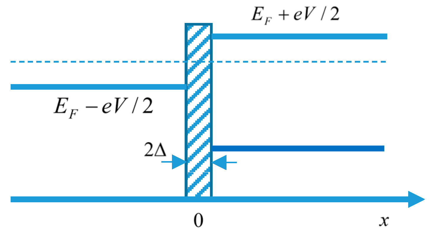
Initially, the particles on the left reservoir occupy all states within the range
, and on the right one, they occupy all states whose energy is within the range
(see
Figure 1). It is taken that the temperature is close to zero.
The eigenstates on the left reservoir are then
for
and on the right one, they are
for
where
is the Heaviside step function,
is the normalization constant, and
is the length of half space.
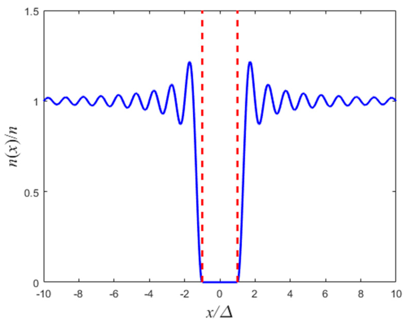
Initially, it follows that the particles’ density is
where
. Therefore, as can be seen in
Figure 2, the shutter repels the particles to a distance
.
3. The Solution
Due to the symmetry of the problem, it is sufficient to investigate the temporal dynamics of the left states. After the barrier is released, i.e., when the potential shutter vanishes, each one of the left eigenstates propagates according to the following:
where
is the Moshinsky function [
6,
7] and erfc is the complementary error function [
19]. Therefore, since
the current density of the single state with the wavenumber
satisfies
where
represents the imaginary part and the asterisks stand for the complex conjugate. Then (following Equations (7)–(10)),
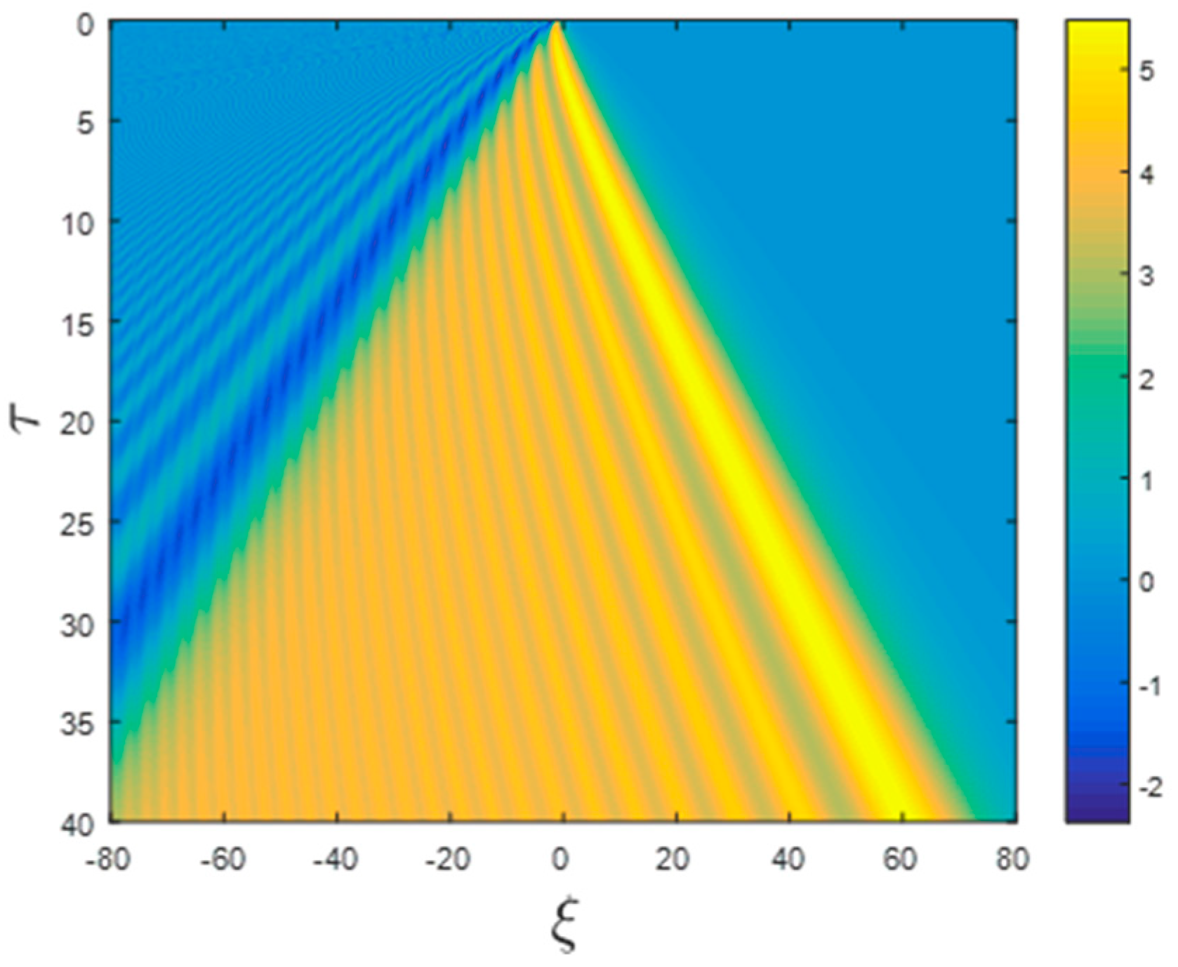
Before we continue to calculate the total current, it is instructive to investigate the dynamics of this single state. For a given wavenumber
, one can define dimensionless parameters,
in which case, the current reveals a universal form
This is a universal pattern, since in terms of the normalized time
and normalized space
, it depends only on a single parameter
, and in the limit of
(i.e., an extremely narrow shutter), the pattern is totally universal. The spatiotemporal structure of this dimensionless current is presented in
Figure 3.
As can be seen from
Figure 3, the current emerges at the transition (singular) point and propagates to both directions, i.e., for a given
, the current is restricted to the regional space
. Beyond these points, there are only ripples, which are also universal, as will be shown below.
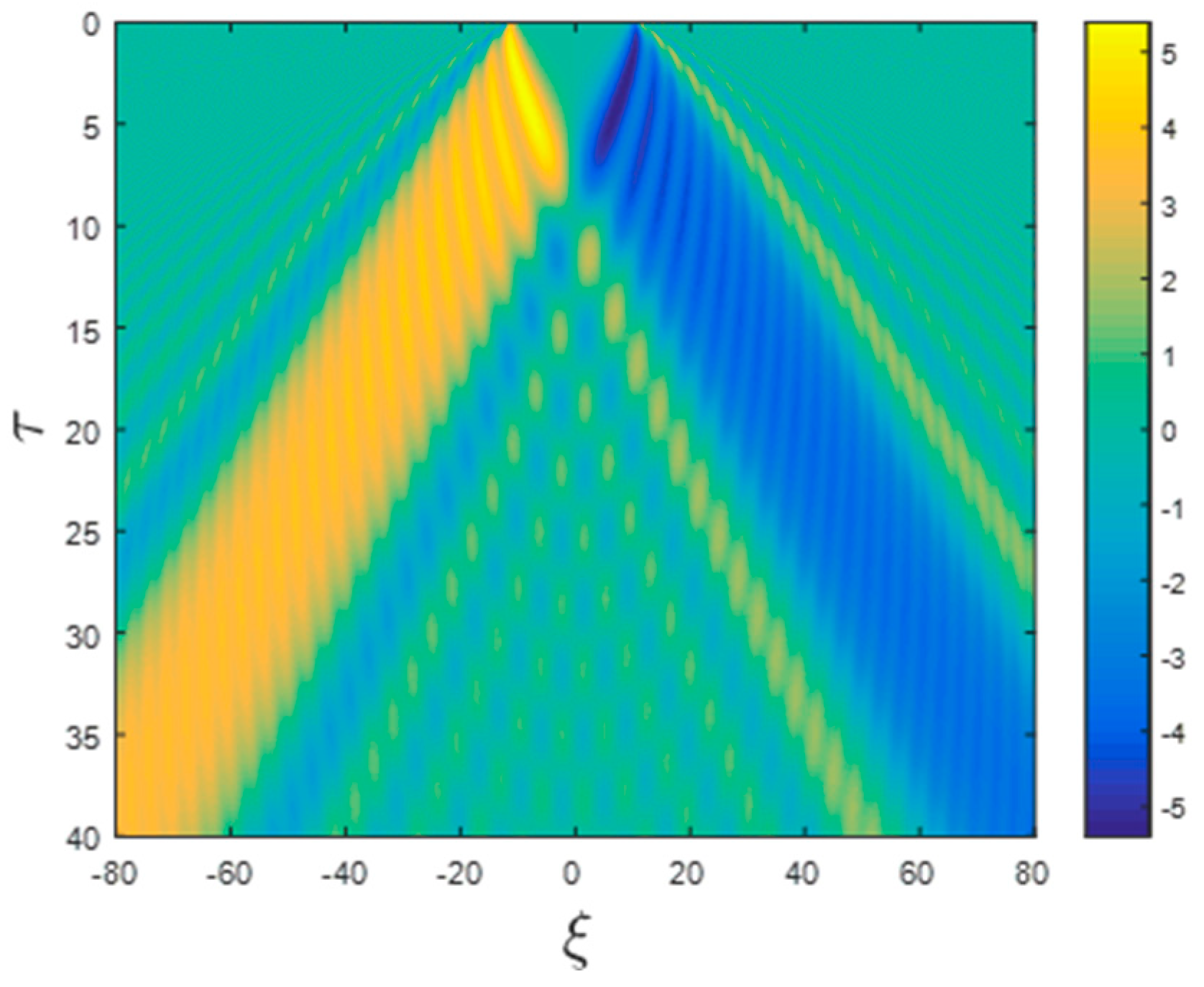
Consequently, there are non-zero currents everywhere. Even when the voltage difference
V is zero, currents are spread all over space when the shutter is lifted, albeit the
average current is zero, and in particular, the current at the shutter’s center, i.e.,
x = 0, is always zero even when it is lifted. Such a case is presented in
Figure 4. Clearly, the ripples exist even when the shutter has zero width (
). A non-zero current emerges at
x = 0 when there is a net voltage difference. At zero temperature, the current reads
where
and
are the maximum wavenumbers of the right and left reservoirs, respectively. The prefactor 2 corresponds to the two spin states.
In the derivation of (14), it was taken that .
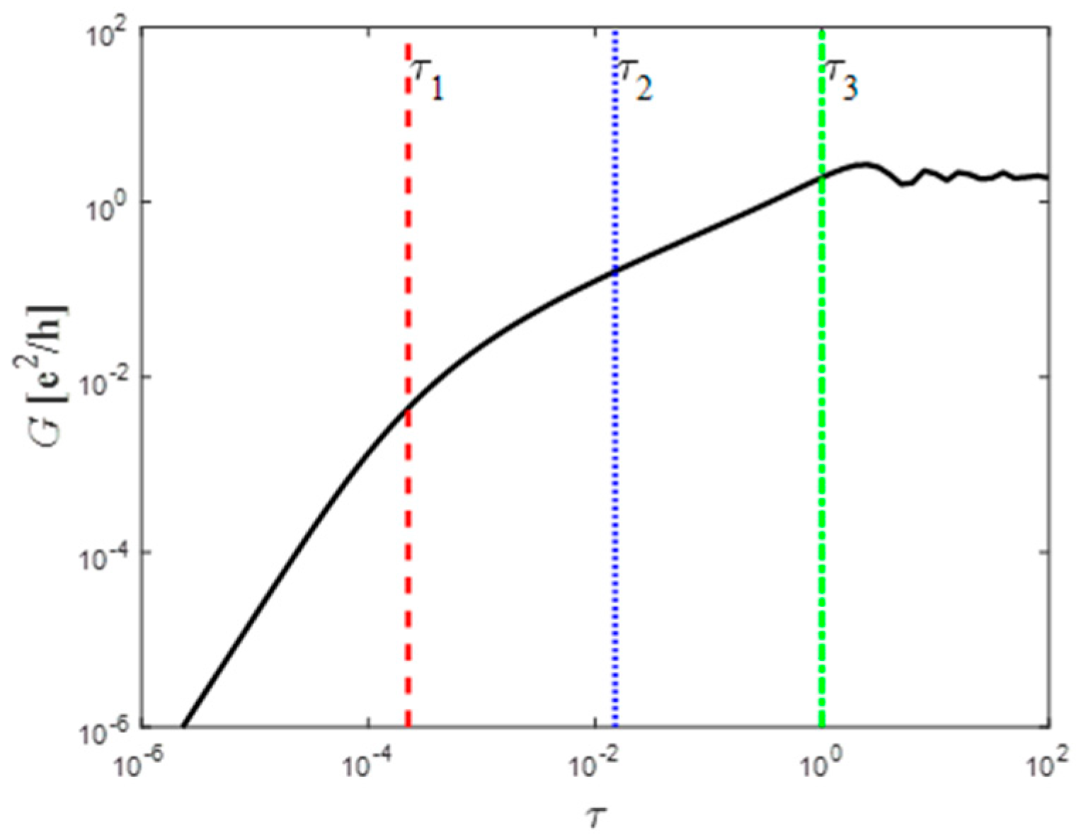
Therefore, the conductance
is time-dependent:
where
can be approximated by the average
.
The system is governed by three relevant time scales:
Since
is the particles’ density (
is the charge density), then the size of
(which can be interpreted as the number of particles that populate a region which is equal to the shutter’s width) determines which length scale is larger. In the low-density scenario,
, then
and vice versa; when
, then
. It is easier to investigate the different time domains using the dimensionless temporal parameters as follows:
It should be pointed out that in the limit
(this is the regime of a narrow shutter, or low density
), Expression (15) turns into a simpler form:
where
and
are the Fresnel C and S integrals [
19] and
represents the real part.
4. Short-Time Behavior
When
is a large number (
), there is only one short-time dynamic. In this case, the conductance rises as
, or more precisely
However, if , the dynamic behavior can vary drastically in the short-time regime.
In
Figure 5, the scenario with
is presented. As can be seen from this figure, the three time scales are clearly shown.
In the very short-time regime, i.e.,
(
), the conductance agrees with Equation (19); however, between the time scales,
(
)
, i.e.,
where, again,
is the particles’ density. In between these temporal behaviors
, there is a gradual transition.
Clearly, when the shutter width goes to zero, Equation (20) is valid as long as , i.e., (20) is valid in the short-time domain.
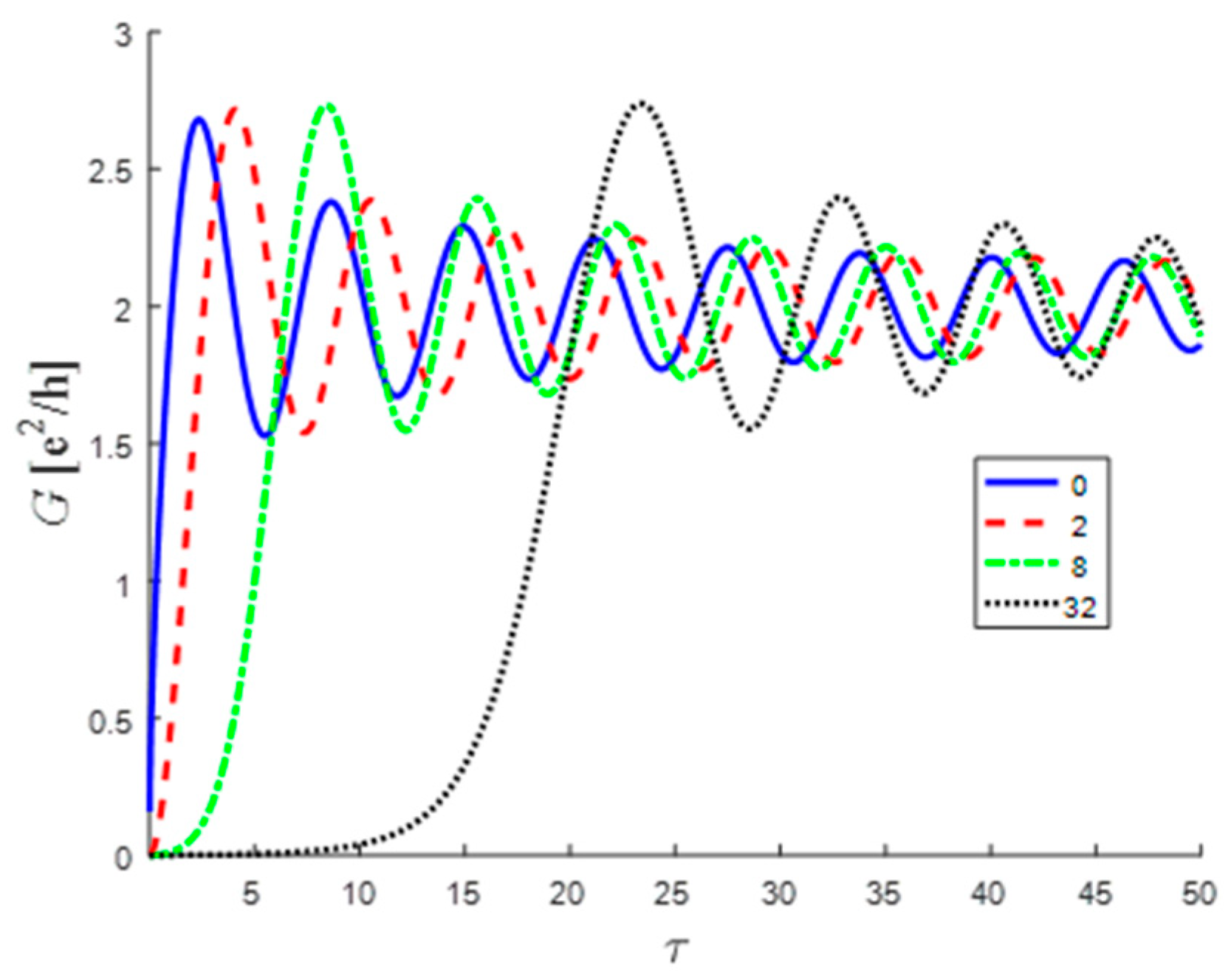
5. Long-Time Behavior
In the long-time regime,
and the current oscillates. In this regime, Expression (15) can be approximated by the following:
where
and
are again the Fresnel C and S integrals, respectively [
19], and
. Equation (21) can be further approximated by the following:
Equation (22) emphasizes the fact that the current oscillates with varying frequency,
which converges to the frequency
The higher the particles’ density, the higher this frequency; however, the rate in which the system converges to equilibrium is independent of the particles density or mass. In the long-time regime,
and eventually, the conductance converges to its well-known equilibrium value
with an oscillation amplitude that decays as
. In this regime, the dependence on the specific properties of the system disappears and the well-known universality reappears.
However, we meet another universal relation between the short-time conductance and the long-time oscillations’ frequency; namely, in the regime of a narrow shutter, we find
Moreover, another universality appears. Initially, unlike the classical analogy, the current is zero and rises monotonically to an overshoot value and only then oscillates and converges to its final value.
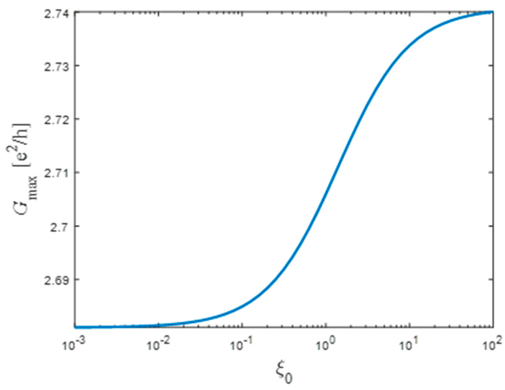
The maximum overshoot current value is dependent on the shutter’s width. However, as can be seen from
Figure 6, the variations are miniscule. In fact, a good approximation of
can be evaluated using the first maximum of (25), i.e., it can be evaluated in the absence of the shutter, in which case
In
Figure 7,
is plotted as a function of the normalized shutter’s width
for five orders of magnitude. In this regime,
varies by less than 3%.
Since the first maximum is reached approximately at
, then the two extreme values can be evaluated by substituting this value into the conductance formula for the two limiting regimes (
and
). The lower value can be evaluated by the following:
and the upper value can be evaluated by the following:
It should be emphasized that this is a local instantaneous conductance which can exceed the equilibrium value (26). This is possible due to an instantaneous increase in the particles’ density (see
Figure 2) followed by a similar decrease in the particles’ density. Consequently, on average, the equilibrium value is restored.
Furthermore, the average value is almost exactly equal to Euler’s number .
6. Quantum Wire in 3D
The above equations were derived using the single particle 1D Schrödinger equation. In reality, the channel is a thin wire in 3D, and in general, electron–electron interaction cannot be neglected. However, most of the conclusions of the 1D scenario are still valid.
When the wire’s width (
w) is very narrow, i.e.,
, then only the first mode is propagating, and the other modes do not contribute to the current. In which case, the one-electron Schrödinger wavefunction reads
, and the equations for the longitudinal part
and the transverse part can be rewritten as follows:
and
respectively, where
represents the non-linear electron–electron potential,
is the cutoff energy of the wire, and
is the transverse Laplacian.
In general, the solution of (31) is very complex; however, in two time regimes, the non-linear part can be ignored.
In the long-time regime, when only oscillations remain, the system is close to equilibrium, and the oscillations are within the linear regime, in which case can be neglected (theoretically, it should be a constant, which has to be zero to conform with Landauer’s equation) and then Equations (24) and (25) are valid, provided the Fermi energy is reduced by the cutoff energy of the wire, i.e., .
In the short-time regime, the non-linear term can also be neglected, but for a different reason. At
t = 0,
depends analytically on the particles’ density. Therefore, it represents a smooth potential (both its value and its slope are continuous). However, since initially, the wavefunction has a discontinuous derivative at the shutter’s location, the effect of the smooth potential can be neglected in the short-time regime since the wavefunction dynamics are
governed in the short time by the singularity. This phenomenon can be easily understood from the Schrödinger equation (Equation (3)): the temporal change in the wavefunction is governed by two terms—the kinetic term, which is proportional to the second derivative of the wavefunction, and the potential energy term. In the case of a singular wavefunction as in (4), the potential term vanishes continuously at the singular point, while the second derivative diverges at this point. Therefore, in the short-time regime, the effect of the potential term can be ignored in comparison to the kinetic one (for a detailed explanation, see Refs. [
20,
21] and references therein).
Therefore, in the short time that follows the shutter’s removal, the wavefunction singularity governs the wavefunction dynamics, and the non-linear electron–electron interaction can be neglected. Consequently, in the short time, Equation (20) and the square-root temporal behavior are valid, provided the Fermi energy is replaced again with . Moreover, the result of (27), which relates the short-time prefactor to the long-time oscillations, is also valid, even in the physical 3D case where electron–electron interactions are present.
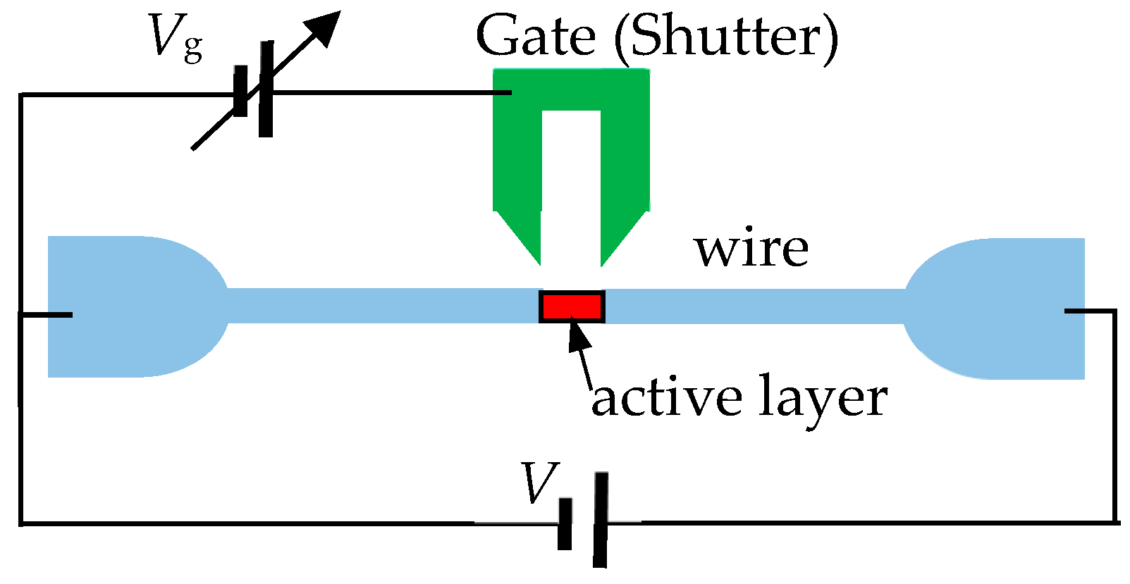
7. Physical Realization
The tunable shutter can be realized as a point of contact with side branches as controls (see, for example, Ref. [
4] and references therein). A schematic illustration of such a system is depicted in
Figure 8. The narrow wire is connected to the active layer, which emits light, and to the voltage source. The gate controls the current from the wire to the active layer, which emits light. The detected light power is proportional to the current through the active layer. If the wire is made of semiconductors, then the Fermi energy is of the order of meV [
4]. Therefore, to prevent multi-mode propagation in the wire, the wire’s width should be around 10–100 nm, where the Fermi energy of the semiconductor is close to the wire’s cutoff energy.
The main difficulty in measuring the short-time behavior is the time response of the active layer, which is of the order of a microsecond. Since the time scale of the system is determined by the effective Fermi energy, the wire should be designed in coordination with the semiconductor’s Fermi energy to keep .
8. Summary
We investigated the currents that emerge when a shutter that distinguishes between adjacent particles’ reservoirs is lifted. Unlike its classical equivalent (and even some quantum ones), the current is initially zero and increases gradually. Initially, the conductance rises like , but beyond a certain time scale, which depends on the shutter’s width, the conductance rises like , where . In the long-time regime, the current oscillates with the same frequency around the universal conductance unit , with an oscillation amplitude that decreases like . Another finding is that the maximum conductance is also universal , where has a weak dependence on the shutter’s width and it is very close to Euler’s number.


