How to Calculate Condensed Matter Electronic Structure Based on Multi-Electron Atom Semi-Classical Model

Abstract

Atoms are proved to be semi-classical electronic systems in the sense of closeness of their exact quantum electron energy spectrum with that calculated within semi-classical approximation. Introduced semi-classical model of atom represents the wave functions of bounded in atom electrons in form of hydrogen-like atomic orbitals with explicitly defined effective charge numbers. The hydrogen-like electron orbitals of constituting condensed matter atoms are used to calculate the matrix elements of the secular equation determining the condensed matter electronic structure in the linear-combination-of-atomic-orbitals (LCAO) approach. Preliminary test calculations are conducted for boron B atom and diboron B₂ molecule electron systems.

1. Introduction

Earlier author developed so-called quasi-classical theory of substance (QCTS), the theoretical method for calculating condensed matter electronic structure quantitative characteristics based on quasi-classical parameterization of electron density and electric field potential distributions in the constituent atoms. Detailed description of the physical theory one can find, e.g., in [1]. As for the resolution of special mathematical problems of this approach, they are summarized in [2,3,4]. Within the initial quasi-classical, i.e., semi-classical, approximation, QCTS represents electron density and electric field potential distributions in atoms by the step-like radial functions [5].

Today the QCTS is implemented mainly for elemental boron and boron nitride species: molecules, clusters, nanostructures, and crystalline modifications. In particular, by this method the values of ground state (chemical bonds length, molar binding energy, localized vibration frequencies, etc.) and electronic structure (electronic density-of-states (DoS) maxima positions, band gap, impurity energy levels, etc.) parameters were calculated [6,7,8,9,10,11,12,13,14,15,16,17,18,19,20,21]; as well as some of isotopic effects in solids were successfully interpreted.

The estimated relative errors of the QCTS in calculating condensed matter energy and structural parameters are expected to be a few percent, which is acceptable for most of materials science problems. When calculations are carried out in theory’s semi-classical limit, there are absent any ambiguous uncertainties in the results. The point is that the step-like presentations of electron density and electric field potential distributions imply the strict finiteness of the atomic radii. For this reason, the infinite series expressing the matrix elements of the secular equation determining electronic structure are converted into sums of a finite number of nonzero terms without artificial termination.

However, advantage of the QCTS to avoid computation uncertainties turns into its disadvantage: the lack of expressions of electric charge density and electric field potential distributions in atoms and their bounded systems, in particular, condensed matter by continuous functions.

The new semi-classical method proposed in this paper should be considered as a higher stage in development of semi-classical approach to the calculation of condensed matter electronic structure.

It is proved that atoms are semi-classical electronic systems in the sense of closeness of their exact quantum spectrum of electronic energies with the spectrum calculated in the semi-classical approximation. On this basis, a semi-classical model of the atom is introduced, within which the potential of self-consistent electric field acting on given atomic electron is represented in the Coulomb-like form with corresponding effective charge number. For chosen electronic configuration of the atom, the consistent set of atomic potentials effective charge number values can be found explicitly by integrating combinations of transcendental functions.

Further, that set of effective charge numbers of atomic potentials is used to construct hydrogen-like atomic orbitals and calculate radii of classical orbits and energies of electrons filling them.

Then hydrogen-like electron orbitals of atoms constituting the condensed matter under consideration are used to calculate the matrix elements of the secular equation determining the condensed matter electronic structure in the linear-combination-of-atomic-orbitals (LCAO) approach.

2. Multi-Electron Atom Semi-Classical Model

There is given a proper justification of basic assumptions of the semi-classical model, which is introduced here for the multi-electron atom taking into account a number of relevant works available in the literature. The assumptions proved are of key importance for semi-classical atomic orbitals and potential constructed below. For their part, semi-classical calculations of the electronic structure of any bound system of atoms, including condensed matter, will be based just on these semi-classical atomic orbitals and potential.

2.1. Stationary State

In atomic nucleus, which is the bounded system of nucleons—protons and neutrons, the presence of at least one proton is obligatory to have non-zero electric charge. As the nucleon in ~2000 times exceeds electron by mass, mass of the electron bounded in atom is almost negligible compared to the total mass of the atomic core, i.e., the bounded system of nucleus and the rest of atomic electrons. By assuming the nucleus mass infinite the atom is imagined as a system of positively charged nucleus fixed in the rest and negatively charged electrons moving around. Each atomic electron is affected by approximately stationary self-consistent-field (SCF) consisted of stationary electric field of the nucleus and time-averaged superposition of electric fields of moving in the corresponding atomic core electrons.

As single-electron wave equation with stationary binding potential leads to discrete energy eigenvalues, the atomic SCF conception reduces the multi-electron atom problem to the determination of its electronic structure—single-electron atomic orbitals (AO) and corresponding electron energy levels.

Thus, the single-electron approximation for multi-electron atoms actually is based on the huge difference (three to five orders of magnitude) of mass between nuclei and electrons making the formers behave similar to classical particles. To establish the single-electron description of the atomic electronic system, one has to start with the exact, i.e., multi-electron, Hamiltonian and introduce approximations, which lead to set of single-electron-like equations for electrons in the external potential created by the presence of atomic nucleus and other electrons [22]. Each electron experiences the presence of other electrons through an effective potential in an approximate way encapsulating the multi-electron nature of the real system. In developing the one-electron picture of atoms, one does not neglect the exchange and correlation effects between electrons but take them into account in an average way usually referred to as a SCF approximation for the electron–electron interactions.

Initially, nonzero relativistic correction to the atomic electron non-relativistic energy level appears only in the second order with respect to the $v/c$ ratio, where $v$ and $c$ are electron and light speeds, respectively. The relativistic correction $~v^2/c^2$ yields so-called fine-structure of the electronic energy spectrum (see, e.g., [23]). It accounts the first-order electron-spin effects as well. As for the correction $~v^3/c^3$, it takes into account the electron radiation, what is incompatible with assumed stationary motion. Thus, it makes no sense to take into account relativistic corrections of orders higher than 2.

In this regard, note that according to the general perturbation theory, any second-order correction to the energy corresponds to first-order correction to the wave function. In addition, since there are no first-order ($~v/c$) relativistic corrections to the atomic energy levels, it should be completely neglected relativistic corrections to the electron wave functions.

Studies show that for the bounded structures of heaviest elements the relativity corrections must be addressed because they strongly affect heavy elements causing complex shifts in their electronic energy levels. For example, two heavy elements, tennessine Ts and oganesson Og, with atomic numbers of 117 and 118, respectively, form pentatomic molecule OgTs₄, which, according to the recent relativistic computations, in tetrahedral geometry is about 1 eV more stable than in square planar geometry [24].

Summarizing, we conclude that the relativistic correction to the atomic electron non-relativistic energy levels should be taken only into the initial nonzero order, which yields the electronic energy spectrum fine-structure and accounts the electron-spin effects as well. As for the relativistic corrections to the electron non-relativistic wave functions, they should be neglected.

2.2. Spherical Symmetry

In the parlance of modern physics, electron is a truly point-like particle. Can one consider the nucleus as material point too? If so, the nucleus fixed in a point serves for source and spherical symmetry center of the Coulomb electric field. As for the intra-atomic SCF, this is too obvious for electron-orbits in light atoms but has never been proven before for low-lying electron-orbits in heavy atoms. To prove the spherical symmetry of intra-atomic SCF in general, we need to evaluate minimum radius of the electron orbits in atom and compare it with maximum electric charge radius of the corresponding atomic nucleus.

Since electrons in low-lying orbits in heavy atoms move with relativistic velocity, non-relativistic analysis is insufficient to estimate the minimum radius of the electron orbits: it is necessary to involve relativistic mechanics. Elsewhere we will give in detail a relativistic generalization (reported in [25]) of the Bohr semi-classical non-relativistic model. According to this generalization, electron orbit radius $r_n$, its velocity in orbit $v_n$, and energy $E_n$ are found from following relations:

$$\frac{r_n}{r_{\mathrm{B}}}=\frac{n^2}{Z}\sqrt{\frac{\sqrt{1+{\beta }_n}+1}{2}}$$

(1)

$$\frac{v_n}{c}=\sqrt{1+\frac{1}{{\beta }_n}}-\sqrt{\frac{1}{{\beta }_n}}$$

(2)

and

$$\frac{E_n}{m{c}^2}=\sqrt{\frac{\sqrt{1+{\beta }_n}+1}{2}}-\frac{1}{2}\sqrt{\frac{{\beta }_n\left(\sqrt{1+{\beta }_n}-1\right)}{2}}$$

(3)

Here,

$$n=1, 2, 3, \dots$$

(4)

is the principal quantum number, while $m$ is the electron rest mass and $Z$ is the nucleus charge number. The electron orbit parameter,

$${\beta }_n=\frac{4{\alpha }^2{Z}^2}{n^2}$$

(5)

is determined by the fine-structure constant,

$$\alpha =\frac{e^2}{\hslash c}\approx \frac{1}{137.04}$$

(6)

And finally,

$$r_{\mathrm{B}}=\frac{{\hslash }^2}{e^{2}m}\approx 0.53 \AA$$

(7)

is the non-relativistic Bohr radius.

On the one hand, at given charge number $Z$ the minimum radius corresponds to the first orbit: $n=1$. On the other hand, the radius of the orbit decreases with increasing in $Z$. If this number is so large that $\alpha Z>1$, i.e., $Z>137$, then the solution of the Dirac relativistic wave equation with the Coulomb potential does not satisfy the physical boundary condition at the center of the field [26]. Resent model [27] of single-electron ion with high accuracy average ionization potential also confirms the thesis about last element of the Periodic Table with $Z=137$. Consequently, the values $Z_{\max }=137$ and ${\beta }_{\max }=4$ are the extremely possible ones for stable atoms. Therefore, we acquire the desired estimate of minimum radius of the relativistic electron orbit in atom:

$$r_{\min }\approx \frac{r_{\mathrm{B}}}{137}\sqrt{\frac{\sqrt{5 }+1}{2}}\approx 0.0049 \AA$$

(8)

It is an underestimated value for $r_{\min }$ because the nuclei themselves become unstable at lower $Z$.

Due to the almost constant density of nuclear matter, the radius of the nucleus was found [28] to be approximately proportional to the cubic root of the atomic number $A$, the sum of numbers of protons $Z$ and neutrons in the nucleus: $R\approx R_A\sqrt[3]{A}$. Here, the averaged value of the proportionality coefficient is: $R_A\approx 0.000012 \AA$. Note that $R$ is the root-mean-square charge radius of the nucleus, not its geometric characteristic. For structurally stable large nuclei $A\approx 2.5 Z$ (see, e.g., [29]) and, consequently,

$$R\approx R_Z\sqrt[3]{Z}$$

(9)

with $R_Z\approx 0.000016 \AA$. Apparently, the estimated nucleus charge radius maximum corresponds to $Z_{\max }=137$:

$$R_{\max }\approx R_Z\sqrt[3]{137}\approx 0.000082 \AA$$

(10)

Thus, the ratio of the maximum possible nucleus charge radius to the minimum electron orbit radius in atoms is much less than 1: $R_{\max }/r_{\min }\approx 0.017\ll 1$. Therefore, even for an extremely heavy nucleus, its charge radius turns out to be significantly smaller compared with the characteristic distance to electron in lowest-lying orbit. For the overwhelming majority of electron-states in atoms with stable nuclei, similar conditions are fulfilled in much better.

The representation of the nucleus as a fixed point electric charge means that the intra-atomic electric SCF is of spherical symmetry with the center at nucleus. The contribution from the nucleus Coulomb-like field directly satisfies this condition. However, as is known the spherical symmetry is not characteristic for electronic contributions. The fact is that the AOs themselves, which are found by solving wave equation with radial potential, are not spherically symmetric: in addition to the radial factor they also contain angular factors. Therefore, to achieve self-consistency, it is necessary that when calculating the atomic SCF the partial electron densities be averaged over directions.

2.3. Semi-Classical Approximation

The semi-classical approximation to quantum mechanics appeared simultaneously with quantum mechanics itself. As early as in his seminal work [30,31,32] Bohr wrote: “… the dynamical equilibrium of the systems in the stationary states can be discussed by help of the ordinary mechanics … assumption seems to present itself; for it is known that the ordinary mechanics cannot have an absolute validity, but will only hold in calculations of certain mean values of the motion of the electrons. On the other hand, in the calculations of the dynamical equilibrium in a stationary state in which there is no relative displacement of the particles, we need not distinguish between the actual motions and their mean values”.

According to the standard quasi-classical, i.e., Wentzel–Kramers–Brillouin (WKB), approximation, in general the particle’s potential energy $U\left(r\right)$ in a stationary radial field has to vary slowly over a distance comparable with its de Broglie wavelength at all the points, where potential energy is negligible in comparison with particle’s total mechanical energy $E$. This criterion certainly cannot be satisfied near the classical turning points, which are determined as roots of the equation: $U\left(r\right)=E$. In the initial, i.e., semi-classical, approximation it leads to so-called connection problem [33], which means searching for the optimal linear combination of semi-classical wave functions well approximating precise one in different regions of the space.

As for atomic potentials, they definitely contradict the mentioned WKB criterion because of Coulomb singularity at the origin and electron-shell structure yielded in the oscillatory radial dependences of electron density and, consequently, potential. For this reason, at first glance the success of the Bohr’s simple semi-classical model giving exact electron energy spectrum for hydrogen-like atoms seems to be partially accidental. The fact is that the electric field bounding single electron with atomic nucleus is purely Coulomb-like and then corresponding wave equation can be solved exactly. In addition, not only for the attracting Coulomb [34], but also for all solvable spherically symmetric potentials [35] application of the standard leading-order in $\hslash$ WKB quantization rule to the wave equation reproduces exact energy spectrum. It also has been argued [36] that contrary to widespread belief, Bohr’s model is consistent and can be interpreted to support the moderate and selective version of the realistic description.

For example, Potapov reported [37] on so-called dipole–shell model of the atom, which can be considered as a neoclassical development of the Bohr’s semi-classical shell-model. In such a way, atom is represented as a classical object—set of nested each in other quasi-spheres or shells formed by circular/elliptical electron orbits. The conceptual basis of this model consists in using the Gauss theorem to reduce the multi-charge problem to the two-charge one. In connection with this work, it must be emphasized that we strongly disagree with author’s claim that a purely classical description, completely neglecting any quantum effects, can give the exhaustive explanation of all the observed atomic phenomena. Potapov’s approach itself being purely classical does not contain any Planck constant dependent quantum correction to the electronic energy levels in atom. Its errors can be revealed in the quantum consideration, namely, by the asymptotic expansion of the electronic energy spectrum showing that even the initial term corresponding to the semi-classical approximation, in the general case, depends on the Planck constant (see below). In [38], for two-electron or helium-like atoms it was demonstrated how to extract useful information about the light atoms electronic structure from their classical study by numerical methods.

Direct extending of the Bohr’s simple semi-classical model to helium-like, i.e., two-electron, atomic systems [39] leads to the renormalization of the nuclear charge number. Obtained in this way ground state energies differ from the experimental ones only in a few percent. Review [40] discussed the modified semi-classical concepts and their application to two-electron atoms offering the viewpoint complementary to numerical quantum-mechanical approach. Interpretations of approximate quantum numbers and rules are given in terms of key periodic orbits of the classical three-body Coulomb problem. The focus lies on the periodic orbit trace formulas able to resolve quantitatively resonances and bound states from the ground state across the two-body fragmentation thresholds.

Bohr-type semi-classical analytical models’ suitability was demonstrated for electron trajectories in small neutral molecules and molecular ions with two or three electrons [41]. In particular, the classical description of periodic motion was shown to be not necessarily limited to cases with $\hslash \to 0$. Other simple extension of the Bohr’s semi-classical molecular model [42] gives a clear physical picture of how electrons create chemical bonds and provides surprisingly accurate ground-state potential energy curves for light diatomic molecules.

To simulate the many-electron systems such as heavy atoms, multi-atomic molecules, and condensed matter, the semi-classical approximation should be combined with statistical one. Even the simplest Thomas–Fermi model [43,44] gives the intra-atomic electron density distribution, which is suitable as initial approximation when interpreting the electromagnetic waves scattering in condensed matter. Based on Thomas–Fermi semi-classical model, a special methodology allows [45] to find single-electron densities even beyond electrons classical turning points in atom and use them for revealing shell-effects characteristic of many-electron quantum systems.

Further development of the semi-classical/statistical approach leads to the class of modified or generalized Thomas–Fermi equations (see, e.g., [46]), which take into account various quantum and statistical corrections introduced by adding corresponding terms in the atom electron system total energy expression. Emphasize that non-relativistic Thomas–Fermi model admits direct relativistic generalization as well.

Perhaps, the most complete and consistent generalization of the Thomas–Fermi model was given by the Magomedov radial-statistical model [47], in which radial electron orbitals corresponding to the semi-classical SCF are introduced for spherical bound multi-electron system such as atom. This approach is equivalent to the Thomas–Fermi model only in the limit of infinite number of electrons in the system. Magomedov model has revealed the loss of the major, first order, correction to Thomas–Fermi model [48], the origin of which is purely statistical. It is associated with the replacement of summation over quantum numbers by integration, when considering them for continuous variables.

The second order correction basically is a statistical one as well because mainly is caused by the Dirac’s electron–electron exchange correction. There are von Weizsacker’s quantum and also so-called shell corrections of the same parametric smallness, but with much smaller numerical coefficients. The introduction of the Amaldi’s third order correction is related to the necessity to exclude the nonphysical effect of electron self-action, i.e., it again is related to the statistical approximation. Thus, errors of the Thomas–Fermi-type approaches are predominantly of statistical origin, not semi-classical one.

Density functional theory (DFT) is the most modern formulation of statistical modeling of multi-electron bounded systems. The density of the total kinetic energy of the electron jellium as a function of electron density permits systematic decomposition into quasi-classical series [49], the initial, semi-classical, approximation of which corresponds to so-called local density approximation (LDA). The well-known success of the LDA once again confirms the suitability of the semi-classical approach to atoms and systems of bounded atoms such as molecules and condensed matter.

As it was mentioned in the Introduction, the errors of the QCTS in semi-classical calculating of condensed matter electron energy and structural parameters do not exceed a few percent.

What is the reason for the successful practice of applying various semi-classical approaches to the problem of isolated atoms and bounded systems of atoms? The key to understanding the semi-classical nature of physical systems seems that in the wave equation the small parameter, Plank constant $\hslash$, stands at highest derivative. Both in non-relativistic and relativistic cases, this allows the asymptotic finding of an approximate solution [50].

Let us consider the motion of a quantum particle along the $x$-axis and assume that its stationary potential energy $U\left(x\right)$ satisfies the following conditions: (1) the spectrum of the corresponding one-dimensional Schrödinger equation near the energy $E$ is purely discrete; (2) there exists a region with $U\left(x\right)-E<0$, the simply connected part of which is bounded by the points $x_1\left(E\right)$ and $x_2\left(E\right)$ representing the simple zeros of the difference $U\left(x\right)-E$; and (3) the function $U\left(x\right)$ is infinitely differentiable. For these conditions that are usually satisfied by physical potentials, Maslov proved theorem [51] on the possibility to represent discrete energy eigenvalues $E_i$ of the stationary one-dimensional Schrödinger equation with a binding potential by asymptotic series in powers of ${\hslash }^2$:

$$E_i={{\displaystyle \sum }}_{k=0}^{k=\infty }{\hslash }^{2k}{E}_i^{\left(k\right)}$$

(11)

where,

$$i=1, 2, 3, \dots$$

(12)

denotes the number of discrete energy levels. It is obvious that the index $i$ is equivalent to a certain set of quantum numbers. Emphasize that, in general, the coefficients $E_i^{\left(k\right)}$ here are not independent of the small parameter $\hslash$. Formally, above expression is similar to the series obtained by the perturbation theory. The fundamental difference between the conditions of applicability of asymptotic expansion and perturbation theory is that in the first case a small parameter is contained in the kinetic part of the Hamiltonian, while in the second case it is in the potential one.

The energy $E_i^{\left(0\right)}$ is determined in the semi-classical approximation—by the standard semi-classical Bohr–Sommerfeld quantization rule. As for the members of higher orders, they are determined by recursive relations. For the terms not only of zero, but also first and second orders, the formulas are obtained in a simple closed form.

Obviously, this theorem can also be extended to the three-dimensional radial Schrödinger equation, if so-called effective potential energy $U_{\mathrm{eff}}\left(r\right)$ is introduced by adding the centrifugal part to the physical one [23]:

$$U_{\mathrm{eff}}\left(r\right)=U\left(r\right)+\frac{{\hslash }^{2}l\left(l+1\right)}{2m{r}^2}$$

(13)

Here $m$ is the mass of the particle and $l$ is its orbital quantum number.

If $U_0$ denotes the characteristic value of the potential energy, and $r_0$ is the characteristic distance of its significant change in magnitude, then one can enter the small dimensionless parameter [23],

$$\eta =\frac{{\hslash }^2}{2m{U}_0{r}_0^2}$$

(14)

by help of which and on the basis of the asymptotic expansion in powers of ${\hslash }^2$, the semi-classicality condition of the discrete energy spectrum of a bounded non-relativistic particle can be formulated as,

$$\eta \ll 1$$

(15)

We call this condition the Maslov criterion.

It should be emphasized that, in general, the discrete energy spectrum semi-classicality condition (15) is not equivalent to standard WKB condition for the wave functions semi-classicality.

It is interesting to find out the semi-classicality criteria for a relativistic bounded particle as well. Note that in the single-particle Hamiltonian, the Planck constant appears only in the particle momentum operator,

$$\widehat{\overrightarrow{p}}=-i\hslash \overrightarrow{\nabla }$$

(16)

Therefore, the semi-classical decomposition of a relativistic Hamiltonian in powers of squared Planck constant ${\hslash }^2$ is essentially equivalent to its quasi-relativistic decomposition in powers of squared momentum operator ${\widehat{\overrightarrow{p}}}^2$. We arrive at the conclusion that the stated above semi-classicality condition for the Schrödinger equation is preserved for the Dirac equation as well. In this case, $m$ should be understood as the rest mass of a relativistic particle.

Now we can evaluate the Maslov semi-classicality criterion fulfillment specifically for atoms. Since atom is a spherically symmetric bounded system, it is possible to introduce some finite atomic radius $r_{\mathrm{a}}$. In general, the concept of “atomic radius” is not strictly defined. It is a characteristic distance from the nucleus, beyond which the electron density is almost zero. Using this parameter, the potential energy $U_{\mathrm{a}}\left(r\right)$ of given electron in the field of the corresponding atomic core can be represented in the Hartree form (see, e.g., [52]):

$$U_{\mathrm{a}}\left(r\right)=-\frac{e^{2}Z}{r_{\mathrm{a}}}\frac{f\left(r/r_{\mathrm{a}}\right)}{r/r_{\mathrm{a}}}$$

(17)

where,

$$0\le f\left(r/r_{\mathrm{a}}\right)\le 1$$

(18)

is the screening factor of the positively charged nucleus field by the negatively charged cloud of core electrons. Obviously, for the atomic potential,

$$r_0\approx r_{\mathrm{a}}$$

(19)

and then,

$$U_0\approx \frac{e^{2}Z}{r_{\mathrm{a}}}$$

(20)

Consequently, semi-classicality parameter ${\eta }_{\mathrm{a}}$ of the atom is,

$${\eta }_{\mathrm{a}}=\frac{1}{2Z}\frac{r_{\mathrm{B}}}{r_{\mathrm{a}}}$$

(21)

The finiteness of atomic radii is theoretically argued both by first-principle calculations and statistical models. First-principle calculations reveal the fast (exponential) decrease in the electron density at large distance from nucleus, and statistical models of the neutral atom, in which the non-physical effect of the electron self-action is correctly eliminated, explicitly lead to the finite radius.

As for the experimental atomic radii, they are found from the interatomic distances in their structures. Therefore, depending on corresponding interaction nature so-called van der Waals, metal, covalent, and ionic radii can be defined. For the problem under consideration, it is advisable to use the first of them since the van der Waals interaction implies almost only physical contact between the outer electron shells of the neighboring in the structure atoms excluding chemical bonding through valence electrons collectivization or interatomic exchange and transfer.

Table 1. Semi-classicality parameter of neutral atoms.

Atom	$\mathbf{Nucleus} \mathbf{Charge} \mathbf{Number}, \mathit{Z}$	$\mathbf{Van} \mathbf{der} \mathbf{Waals} \mathbf{Radius} {\mathit{r}}_{\mathit{a}}, \AA$	$\mathbf{Semi-Classicality} \mathbf{Parameter}, {\mathit{\eta }}_{\mathit{a}}$
H	1	1.10	0.240
He	2	1.49	0.095
B	5	1.92	0.028
C	6	1.70	0.026
N	7	1.55	0.024
O	8	1.52	0.022
Na	11	2.27	0.011
Fr	87	3.48	0.001

shows the van der Waals radii of some atoms [53] together with the corresponding semi-classicality parameter estimates.

For hydrogen H atom having the smallest radius, the semi-classicality criterion is not very well satisfied. However, it does not matter since the Coulomb potential is exactly solvable and, therefore, its semi-classical electron energy spectrum perfectly coincides with the exact one. As for the next element, helium He, mentioned criterion is satisfied much better. For francium atom Fr with largest radius among all the chemical elements, the satisfaction of semi-classicality criterion is too good. In addition to these extreme cases, Table 1 shows the parameters of atoms B, C, N, O, and Na, the bounded structures of which were semi-classically calculated within the QCTS. It can be seen that for them the semi-classicality condition is fulfilled quite satisfactorily.

Summarizing we conclude that atoms are semi-classical electronic systems in the sense of Maslov criterion. From above numerical estimates, the typical relative differences between semi-classical and exact electron energy spectra for light atoms are <3% and even less for heavy atoms. Thus, the expected accuracy of semi-classical electronic structure calculations for bound system of atoms—molecules and condensed matter—seem to be acceptable in some specific cases.

2.4. Construction of Semi-Classical Atomic Orbitals and Potential

Below, the term “atom” is understood not only as isolated neutral atom or atomic ion, but also as any atom-like particle, i.e., bounded system of a nucleus and one or more electrons constituting some bounded system of atoms—molecule or condensed matter.

Consider the atom containing nuclei with charge number of $Z$ and $N$ electrons. Number electrons by the index $i$:

$$i=1, 2, 3, \dots , N$$

(22)

which is equivalent to the set of atomic quantum numbers:

$$\left(i\right)=\left(n_i, l_i, m_i\right)$$

(23)

Here $n_i$, $l_i$, and $m_i$ are electron $i$-state principal, orbital, and magnetic quantum numbers, respectively. Denote the corresponding discrete electron energy levels by $E_i^{\pm }$ with $E_i^{+}$ and $E_i^{-}$ standing for two different orientations of the electron spin.

Since electrons motion in the atom can be assumed to be semi-classical, most of the time given $i$-electron should be near the surface of the sphere with certain radius $r_i$. In other words, it is possible to assume that its radial coordinate $r$ is a nearly constant quantity:

$$r\approx r_i$$

(24)

By the Gauss theorem, the stationary radial electric field on the spherical surface equals to Coulomb field created by point charge located at the center, the value of which is determined by the sum of electric charges inside this sphere. Therefore, the semi-classical potential energy $U_i\left(r\right)$ of an atomic electron can be approximated in the Coulomb-shaped form:

$$U_i\left(r\right)\approx -\frac{e^2{Z}_i}{r}$$

(25)

where for $i$-electron the relation,

$$Z_i=Z-4\pi {{\displaystyle \sum }}_{i\ne k=1}^{i\ne k=N}{{\displaystyle \int }}_0^{r_i}dr{r}^2{\rho }_k\left(r\right)$$

(26)

determines the effective charge number $Z_i$ of the nucleus shielded by all other atomic electrons. Here functions ${\rho }_i\left(r\right)$ are the radial distributions of partial electron densities in atom. Sum does not contain term with index $k=i$ to avoid inclusion of the $i$-electron self-action non-physical effect.

Approximating the electric field potentials acting on atomic electrons in the Coulomb-like form is too convenient because Coulomb potential is exactly solvable and, therefore, it is possible to find analytical expressions for partial electron density functions ${\rho }_i\left(r\right)$, parameters $r_i$ and $E_i^{\pm }$ and, in this way, finally calculate the effective charge numbers $Z_i$.

As mentioned above, within the SCF approach electron orbits radii and energy levels should be determined in non- and quasi-relativistic approximations, respectively [23]:

$$r_i=\frac{{\hslash }^2{n}_i^2}{e^{2}m{Z}_i}$$

(27)

and

$$E_i^{\pm }=-\frac{e^{4}m{Z}_i^2}{2{\hslash }^2{n}_i^2}-\frac{e^{8}m{Z}_i^4}{2{\hslash }^4{c}^2{n}_i^3}\left(\frac{1}{\left|l_i\pm \frac{1}{2}\right|+\frac{1}{2}}-\frac{3}{4n_i}\right)$$

(28)

The corresponding explicit semi-classical electron AOs ${\psi }_i(\overrightarrow{r})$ are:

$${\psi }_i(\overrightarrow{r})=Y_i\left(\theta ,\phi \right)R_i\left(r\right)$$

(29)

where radius $0\le r\le \infty$, and azimuthal $0\le \theta \le \pi$ and polar $0\le \phi \le 2\pi$ angles are the spherical coordinates.

In general, angular part of the wave function corresponding to a spherically symmetric potential is expressed as a spherical harmonic $Y_i\left(\vartheta ,\phi \right)$ normalized by the condition:

$${{\displaystyle \int }}_0^{\pi }d\theta \sin \theta {{\displaystyle \int }}_0^{2\pi }d\phi {\left|Y_i\left(\theta ,\phi \right)\right|}^2=1$$

(30)

Consequently, wave functions radial parts,

$$R_i\left(r\right)=\frac{2Z_i}{n_i^2{r}_{\mathrm{B}}}\sqrt{\frac{\left(n_i-l_i-1\right)! }{\left(n_i+l_i\right)! }\frac{Z_i}{r_{\mathrm{B}}}}\exp \left(-\frac{Z_{i}r}{n_i{r}_{\mathrm{B}}}\right){\left(\frac{2Z_{i}r}{n_i{r}_{\mathrm{B}}}\right)}^{l_i}{L}_{n_i-l_i-1}^{2l_i+1}\left(\frac{2Z_{i}r}{n_i{r}_{\mathrm{B}}}\right)$$

(31)

which are the real functions expressed by generalized Laguerre polynomials $L_{n_i-l_i-1}^{2l_i+1}\left(2Z_{i}r/n_i{r}_{\mathrm{B}}\right)$, have to satisfy the following normalization condition:

$${{\displaystyle \int }}_0^{\infty }dr{r}^2{R}_i^2\left(r\right)=1$$

(32)

Then, the averaged on full solid angle $4\pi$ partial electron densities are:

$${\rho }_i\left(r\right)=\frac{R_i^2\left(r\right)}{4\pi }$$

(33)

As for the effective charge numbers, now they take the form,

$$Z_i=Z-{{\displaystyle \sum }}_{i\ne k=1}^{i\ne k=N}{{\displaystyle \int }}_0^{r_i}dr{r}^2{R}_k^2\left(r\right)$$

(34)

Let us introduce the new variable,

$$x=\frac{2Z_{i}r}{n_i{r}_{\mathrm{B}}}$$

(35)

which at $r=r_i$ equals to,

$$x_i=2n_i$$

(36)

Thus, the squared semi-classical radial orbital $R_i^2\left(r\right)$ can be rewritten as,

$$R_i^2\left(r\right)=\frac{4Z_i^3}{n_i^4{r}_{\mathrm{B}}^3}\frac{\left(n_i-l_i-1\right)!}{\left(n_i+l_i\right)!}\exp \left(-x\right)x^{2l_i}{\left(L_{n_i-l_i-1}^{2l_i+1}\left(x\right)\right)}^2$$

(37)

We come to the effective charge numbers,

$$Z_i=Z-{{\displaystyle \sum }}_{i\ne k=1}^{i\ne k=N}\frac{\left(n_k-l_k-1\right)!}{2n_k\left(n_k+l_k\right)!}{{\displaystyle \int }}_0^{2n_i}dx\exp \left(-x\right)x^{2\left(l_k+1\right)}{\left(L_{n_k-l_k-1}^{2l_k+1}\left(x\right)\right)}^2$$

(38)

Electron configuration chosen for the atom should be considered as stable if all the charge numbers found in this way are physically meaningful, i.e., positive: $Z_i>0$.

In the full atomic radial potential in sense of potential energy of an electron in atomic SCF,

$$U_{Z Z_1\cdots Z_N}\left(r\right)=U_Z\left(r\right)+U_{Z_1\cdots Z_N}\left(r\right)$$

(39)

the nucleus’ Coulomb potential,

$$U_Z\left(r\right)=-\frac{e^{2}Z}{r}$$

(40)

is added with electron cloud potential $U_{Z_1\cdots Z_N}\left(r\right)$ determined by the Poisson’s equation,

$$\frac{1}{r^2}\frac{d}{dr}\left(r^2\frac{d{U}_{Z_1\cdots Z_N}\left(r\right)}{dr}\right)=-e^2{{\displaystyle \sum }}_{i=1}^{i=N}{R}_i^2\left(r\right)$$

(41)

or in the integral form,

$$U_{Z_1\cdots Z_N}\left(r\right)=-{{\displaystyle \sum }}_{i=1}^{i=N}\frac{e^2{Z}_i}{r_{\mathrm{B}}}\frac{\left(n_i-l_i-1\right)!}{n_i^2\left(n_i+l_i\right)!}{\displaystyle \int }\frac{dr}{r^2}{\displaystyle \int }dr \exp \left(-\frac{2Z_{i}r}{n_i{r}_{\mathrm{B}}}\right){\left(\frac{2Z_{i}r}{n_i{r}_{\mathrm{B}}}\right)}^{2\left(l_i+1\right)}{\left(L_{n_i-l_i-1}^{2l_i+1}\left(\frac{2Z_{i}r}{n_i{r}_{\mathrm{B}}}\right)\right)}^2$$

(42)

As the effective charge number $Z_i$ of a multi-electron atom nucleus for $i$-electron is determined by the sum self-consistent charge density distribution of other atomic electrons, it takes into account electron–electron exchange and correlation effects. It is why in the semi-classical approach (in contrast with, e.g., Hartree–Fock method) there is no need to introduce a correction for electron correlations.

3. Formulation of LCAO Method with Semi-Classical AOs

In the condensed matter, only a part of electrons of constituting atoms called as valence electrons are actually involved in the formation of interatomic bonds, whereas the rest of electrons called as core electrons together with nuclei remain in states almost indistinguishable from their states in corresponding isolated atoms. Therefore, atoms largely retain their individuality within the condensed matter and its treatment as a structure of atom-like systems is acceptable.

This fact explains the successful examples of theoretical description of the condensed matter electronic structure by the LCAO method—see, e.g., [54] (for the origins see [55,56]), which is looking for the electronic subsystem wave function as a linear combination of atom-like orbitals. Both the accuracy and range of applicability of the LCAO method are greatly dependent of effective expression of the set of constituent atoms electronic orbitals used in the trail. Since the standard first principle quantum-chemical methods give AOs in numerical form, the matrix elements of the secular equation determining the condensed matter electronic structure in the LCAO approach usually have to be found by numerical integration as well.

In the previous section, semi-classical electron orbitals are obtained analytically—in form of hydrogen-like atomic orbitals as combinations of generalized Laguerre polynomials and spherical harmonics. Thus, the LCAO method version using hydrogen-like semi-classical atomic orbitals for basis set is expected to determine crystal electronic structure with a good accuracy.

In this section, for simplicity the LCAO method with basic set of semi-classical AOs is introduced for crystals. Formulation can be easily extended to finite clusters or disordered condensed matter by restricting with a single unit cell or substituting periodic lattice by some non-periodic infinite distribution of atomic sites, respectively.

3.1. Formulation of LCAO Method for Semi-Classical Crystal Potential

Crystal single-electron wave functions ${\Psi }_n(\overrightarrow{k},\overrightarrow{r})$ are determined by the stationary Schrödinger equation,

$$\widehat{H}(\overrightarrow{r}){\Psi }_n(\overrightarrow{k},\overrightarrow{r})=E_n(\overrightarrow{k}){\Psi }_n(\overrightarrow{k},\overrightarrow{r})$$

(43)

with non-relativistic Hamiltonian,

$$\widehat{H}(\overrightarrow{r})=-\frac{{\hslash }^2∆}{2m}+U(\overrightarrow{r})$$

(44)

Here $\overrightarrow{r}$ and $\overrightarrow{k}$ are the electron radius- and wave-vectors, respectively; and $m$ is the electron mass.

So-called band approximation means that crystal potential $U(\overrightarrow{r})$ invariant for all the crystal symmetry transformations is a given periodic function of the radius-vector $\overrightarrow{r}$. Here $n$ numbers the electron energy bands $E_n(\overrightarrow{k})$, which are periodic functions of the wave-vector $\overrightarrow{k}$.

In general, three factors determine the applicability of the single-electron approximation to the crystal multi-electron system [57]: (1) range of the electron–electron interactions, (2) electron density, and (3) degree of localization of the constituent electrons. This approximation works better to justifiably construct the single-electron potential for crystals containing a high concentration of significantly delocalized electrons with long-range interactions. In addition, there are two physically different first principles SCF approaches to the single-electron approximation used to arrive at crystal potential: Hartree–Fock method and DFT. First of them considers the electronic wave function, while the second the electron density as primary quantities to be determined.

Solutions can be always written in the form of Bloch functions:

$${\Psi }_n(\overrightarrow{k},\overrightarrow{r})=\frac{1}{\sqrt{N}}{\displaystyle \sum }_{\overrightarrow{\tau }}\exp (i\overrightarrow{k}\overrightarrow{\tau })W_n(\overrightarrow{r}-\overrightarrow{\tau })$$

(45)

where sum is over lattice translations vector $\overrightarrow{\tau }$. $W_n(\overrightarrow{r}-\overrightarrow{\tau })$ indicate Wannier functions localized on corresponding unit cell and $N$ is the total number of unit cells in the crystal. In turn, Wannier functions are expressed by sums over wave vectors $\overrightarrow{k}$ of the Brillouin zone:

$$W_n(\overrightarrow{r}-\overrightarrow{\tau })=\frac{1}{\sqrt{N}}{\displaystyle \sum }_{\overrightarrow{k}}\exp (-i\overrightarrow{k}\overrightarrow{\tau }){\Psi }_n(\overrightarrow{k},\overrightarrow{r})$$

(46)

Wannier functions form an orthonormal set:

$${\displaystyle \int }{d}^3\overrightarrow{r}{W}_{n^{\prime }}^{\ast }(\overrightarrow{r}-{\overrightarrow{\tau }}^{\prime })W_n(\overrightarrow{r}-\overrightarrow{\tau })={\delta }_{n^{\prime }n}{\delta }_{{\overrightarrow{\tau }}^{\prime }\overrightarrow{\tau }}$$

(47)

Let ${\psi }_{i_{\mu }\mu }(\overrightarrow{r}-{\overrightarrow{d}}_{\mu })$ indicates the atomic-like (neutral atom or atomic ion) electron orbital with quantum numbers $i_{\mu }$ for the atom located in position ${\overrightarrow{d}}_{\mu }$ of the unit cell. AOs of any atom form an orthonormal set of basic functions:

$${\displaystyle \int }{d}^3\overrightarrow{r}{\psi }_{i_{\mu }^{\prime }\mu }^{\ast }(\overrightarrow{r}-{\overrightarrow{d}}_{\mu }){\psi }_{i_{\mu }\mu }(\overrightarrow{r}-{\overrightarrow{d}}_{\mu })={\delta }_{i_{\mu }^{\prime }{i}_{\mu }}$$

(48)

Define the corresponding Bloch sum of wave-vector $\overrightarrow{k}$ as:

$${\Phi }_{i_{\mu }\mu }(\overrightarrow{k},\overrightarrow{r})=\frac{1}{\sqrt{N}}{\displaystyle \sum }_{\overrightarrow{\tau }}\exp (i\overrightarrow{k}\overrightarrow{\tau }){\psi }_{i_{\mu }\mu }(\overrightarrow{r}-{\overrightarrow{d}}_{\mu }-\overrightarrow{\tau })$$

(49)

Since any Wannier function $W_n(\overrightarrow{r}-\overrightarrow{\tau })$ can be presented as a LCAO, the crystal wave function can be expressed as linear combination of Bloch sums, i.e., a complete basic set of functions, with same wave-vector:

$${\Psi }_n(\overrightarrow{k},\overrightarrow{r})={\displaystyle \sum }_{\mu }{\displaystyle \sum }_{i_{\mu }}{C}_{i_{\mu }\mu }(\overrightarrow{k}){\Phi }_{i_{\mu }\mu }(\overrightarrow{k},\overrightarrow{r})$$

(50)

Constant coefficients $C_{i_{\mu }\mu }(\overrightarrow{k})$ are determined by requiring that these expansions satisfy the Schrödinger equation. The last is transformed into the secular equation by minimizing the expectation value of the crystal Hamiltonian with respect to coefficients.

Sets of expansion coefficients, which are equivalent to single-electron wave functions, and corresponding electron energies $E$ can be obtained, respectively, as eigenvectors and eigenvalues of the matrix, whose determinantal compatibility equation is

$$det(\langle {\Phi }_{i_{{\mu }^{\prime }}^{\prime }{\mu }^{\prime }}(\overrightarrow{k},\overrightarrow{r})\left|\left(\widehat{H}(\overrightarrow{r})-E(\overrightarrow{k})\right)\right|{\Phi }_{i_{\mu }\mu }(\overrightarrow{k},\overrightarrow{r})\rangle )=0$$

(51)

This secular equation determining the crystal electronic structure contains matrix elements dependent on crystal potential.

It should be noted that, in general, the eigenvalues $E_n(\overrightarrow{k})$ for electronic states ${\Psi }_n(\overrightarrow{k},\overrightarrow{r})$ depend to a large extent on the symmetry properties of the crystal potential $U(\overrightarrow{r})$ used and are not too sensitive to small deviations in its magnitude. This is why in many cases LCAO calculations are qualitatively successful dispute potential’s approximations involved. However, to obtain quantitative results the crystal potential $U(\overrightarrow{r})$ should be constructed properly.

For a good initial approximation to the crystal potential $U(\overrightarrow{r})$ usually it is considered superposition of centered at lattice sites spherically symmetric atom-like potentials $U_{\mu }(|\overrightarrow{r}-{\overrightarrow{d}}_{\mu }-\overrightarrow{\tau }|)$, which are derived from self-consistent potentials of corresponding atoms in their free states:

$$U(\overrightarrow{r})\approx {\displaystyle \sum }_{\overrightarrow{\tau }}{\displaystyle \sum }_{\mu }{U}_{\mu }(|\overrightarrow{r}-{\overrightarrow{d}}_{\mu }-\overrightarrow{\tau }|)$$

(52)

To obtain most accurate presentation for crystal potential, in electron state calculations attempts are made to achieve self-consistency by successively and iteratively recomputing the crystal potential from the multi-electron wave function of the crystal.

In previous section, it has been calculated the semi-classical atom-like radial potentials providing good accuracy for crystal potential constructed as their superposition.

3.2. Calculation of Semi-Classical Matrix Elements

Historically, one had to choose a set of basic functions so that to obtain meaningful results with a small number terms in the expressions. In the tight binding approximation (see, e.g., [58]), the crudest version of the LCAO method, interactions only between nearest neighbor and next to nearest neighbor atoms are taken into account. However, for today computers, the calculation of arising, for example, in the LCAO approach quantum-chemical integrals with the required accuracy is not a principal problem [59]. Though, band structural calculations remain generally quite laborious.

The semi-classical atomic orbital ${\psi }_{i_{\mu }\mu }(\overrightarrow{r}-{\overrightarrow{d}}_{\mu }-\overrightarrow{\tau })$ satisfies Schrödinger equation,

$$\widehat{H}(\overrightarrow{r}){\psi }_{i_{\mu }\mu }(\overrightarrow{r}-{\overrightarrow{d}}_{\mu }-\overrightarrow{\tau })=-\frac{{\hslash }^2}{2m}\frac{d^2{\psi }_{i_{\mu }\mu }(\overrightarrow{r}-{\overrightarrow{d}}_{\mu }-\overrightarrow{\tau })}{d{\overrightarrow{r}}^2}-\frac{e^2{Z}_{i_{\mu }}}{|\overrightarrow{r}-{\overrightarrow{d}}_{\mu }-\overrightarrow{\tau }|}{\psi }_{i_{\mu }\mu }(\overrightarrow{r}-{\overrightarrow{d}}_{\mu }-\overrightarrow{\tau })=E_{i_{\mu }}^{\pm }{\psi }_{i_{\mu }\mu }(\overrightarrow{r}-{\overrightarrow{d}}_{\mu }-\overrightarrow{\tau })$$

(53)

It makes possible matrix element decomposition into two terms:

$$\begin{gathered} \langle {\Phi }_{i_{{\mu }^{\prime }}^{\prime }{\mu }^{\prime }}(\overrightarrow{k},\overrightarrow{r})\left|\left(\widehat{H}(\overrightarrow{r})-E(\overrightarrow{k})\right)\right|{\Phi }_{i_{\mu }\mu }(\overrightarrow{k},\overrightarrow{r})\rangle = \\ =\langle {\Phi }_{i_{{\mu }^{\prime }}^{\prime }{\mu }^{\prime }}(\overrightarrow{k},\overrightarrow{r})\left|\left(U(\overrightarrow{r})+\frac{e^2{Z}_{i_{\mu }}}{|\overrightarrow{r}-{\overrightarrow{d}}_{\mu }-\overrightarrow{\tau }|}\right)\right|{\Phi }_{i_{\mu }\mu }(\overrightarrow{k},\overrightarrow{r})\rangle +\left(E_{i_{\mu }}^{\pm }-E(\overrightarrow{k})\right)\langle {\Phi }_{i_{{\mu }^{\prime }}^{\prime }{\mu }^{\prime }}(\overrightarrow{k},\overrightarrow{r})|{\Phi }_{i_{\mu }\mu }(\overrightarrow{k},\overrightarrow{r})\rangle \end{gathered}$$

(54)

The second, simpler, term is proportional to the overlap integral between two Bloch sums:

$$\begin{gathered} I_{i_{{\mu }^{\prime }}^{\prime }{i}_{\mu }}=\langle {\Phi }_{i_{{\mu }^{\prime }}^{\prime }{\mu }^{\prime }}(\overrightarrow{k},\overrightarrow{r})|{\Phi }_{i_{\mu }\mu }(\overrightarrow{k},\overrightarrow{r})\rangle = \\ =\frac{1}{N}{\displaystyle \sum }_{\overrightarrow{\tau }}{\displaystyle \sum }_{{\overrightarrow{\tau }}^{\prime }}\exp \left(i\overrightarrow{k}(\overrightarrow{\tau }-{\overrightarrow{\tau }}^{\prime })\right){\displaystyle \int }{d}^3\overrightarrow{r}{\psi }_{i_{{\mu }^{\prime }}^{\prime }{\mu }^{\prime }}^{\ast }(\overrightarrow{r}-{\overrightarrow{d}}_{{\mu }^{\prime }}-{\overrightarrow{\tau }}^{\prime }){\psi }_{i_{\mu }\mu }(\overrightarrow{r}-{\overrightarrow{d}}_{\mu }-\overrightarrow{\tau })= \\ ={\displaystyle \sum }_{\overrightarrow{\tau }}\exp (i\overrightarrow{k}\overrightarrow{\tau }){\displaystyle \int }{d}^3\overrightarrow{r}{\psi }_{i_{{\mu }^{\prime }}^{\prime }{\mu }^{\prime }}^{\ast }(\overrightarrow{r}-{\overrightarrow{d}}_{{\mu }^{\prime }}){\psi }_{i_{\mu }\mu }(\overrightarrow{r}-{\overrightarrow{d}}_{\mu }-\overrightarrow{\tau }) \end{gathered}$$

(55)

Here summation over translations vector ${\overrightarrow{\tau }}^{\prime }$ cancels the factor $1/N$. This term contains one- and two-center integrals. The one-center integrals are simply 1 or 0 because orthonormal properties of atomic orbitals set. As for the two-center integrals at given interatomic distances, they are reducible to a smaller number if independent ones. In semi-classical approximation, overlap matrix elements are expressed through special functions—spherical harmonics and generalized Laguerre polynomials—integrals.

The first, more complex, term,

$$\begin{gathered} U_{i_{{\mu }^{\prime }}^{\prime }{i}_{\mu }}=\langle {\Phi }_{i_{{\mu }^{\prime }}^{\prime }{\mu }^{\prime }}(\overrightarrow{k},\overrightarrow{r})\left|\left(U_{i_{\mu }\mu \overrightarrow{\tau }}(\overrightarrow{r})\right)\right|{\Phi }_{i_{\mu }\mu }(\overrightarrow{k},\overrightarrow{r})= \\ =\frac{1}{N}{\displaystyle \sum }_{\overrightarrow{\tau }}{\displaystyle \sum }_{{\overrightarrow{\tau }}^{\prime }}\exp \left(i\overrightarrow{k}(\overrightarrow{\tau }-{\overrightarrow{\tau }}^{\prime })\right){\displaystyle \int }{d}^3\overrightarrow{r}{\psi }_{i_{{\mu }^{\prime }}^{\prime }{\mu }^{\prime }}^{\ast }(\overrightarrow{r}-{\overrightarrow{d}}_{{\mu }^{\prime }}-{\overrightarrow{\tau }}^{\prime })\left(U(\overrightarrow{r})+\frac{e^2{Z}_{i_{\mu }}}{\left|\overrightarrow{r}-{\overrightarrow{d}}_{\mu }-\overrightarrow{\tau }\right|}\right){\psi }_{i_{\mu }\mu }(\overrightarrow{r}-{\overrightarrow{d}}_{\mu }-\overrightarrow{\tau })= \\ ={\displaystyle \sum }_{\overrightarrow{\tau }}\exp (i\overrightarrow{k}\overrightarrow{\tau }){\displaystyle \int }{d}^3\overrightarrow{r}{\psi }_{i_{{\mu }^{\prime }}^{\prime }{\mu }^{\prime }}^{\ast }(\overrightarrow{r}-{\overrightarrow{d}}_{{\mu }^{\prime }})\left(U(\overrightarrow{r})+\frac{e^2{Z}_{i_{\mu }}}{\left|\overrightarrow{r}-{\overrightarrow{d}}_{\mu }-\overrightarrow{\tau }\right|}\right){\psi }_{i_{\mu }\mu }(\overrightarrow{r}-{\overrightarrow{d}}_{\mu }-\overrightarrow{\tau }) \end{gathered}$$

(56)

is the matrix element between two Bloch sums of crystal potential minus semi-classical potential acting on electron in given atomic state:

$$U_{i_{\mu }\mu \overrightarrow{\tau }}(\overrightarrow{r})=U(\overrightarrow{r})+\frac{e^2{Z}_{i_{\mu }}}{|\overrightarrow{r}-{\overrightarrow{d}}_{\mu }-\overrightarrow{\tau }|}$$

(57)

It contains two- and three-center integrals. Here the three-center integrals, similar to the two-center integrals, for given interatomic distances can be reduced to a smaller number of independent ones. In semi-classical approximation, potential matrix elements are expressed through same special functions integrals.

4. Test Calculations

The numerical realization of the introduced semi-classical method needs a number of further studies: (1) Computing and tabulating of effective nucleus charge numbers for semi-classical electron orbitals and corresponding radii of electron orbits and electron energy levels in stable neutral atoms and atomic ions in their isolated states; (2) Constructing of semi-classical atomic (ionic) potentials; (3) Reducing of the semi-classical secular equation matrix elements to the linear combinations of irreducible one-, two-, and three-center overlap and potential energy integrals expressed analytically in special functions; and (4) Solving the secular equation to determine electron energy spectrum and electron density distribution of substances—bounded system of atoms.

Here we aim to conduct only a preliminary numerical testing of the proposed semi-classical method. In addition, to simplify its procedure as possible, we make several additional assumptions:

-

Consider elemental substance, namely boron B, not a compound of two or more chemical elements.

-

Consider smallest—diatomic molecule B₂, not a crystalline modification of boron.

-

Include into the LCAO basis only higher valence electron orbitals.

-

Conduct calculations in the non-relativistic limit.

To imagine the introduced additional (to proposed semi-classical approach) calculation errors, characterize these assumptions in brief.

As boron is light chemical element, electron orbitals in boron atoms possess low quantum numbers. For common versions of the semi-classical approximation, it is a critical case. In this regard, testing on an all-boron system should provide a quite good evaluation of the accuracy expected for proposed semi-classical method.

Analyzing electronic structure of a small molecule does not affect the calculations accuracy. Furthermore, B₂ molecule or isolated B–B bond is of academic interest because it is considered as “building block” of important boron 3D allotropes and also nanostructures, in particular, boron monoatomic sheet–borophene, which is a new prospective 2D material with properties in many aspects supplementary to that of the well-known and widely used graphene.

As for the restriction with only higher valence-electron orbitals basis in LCAO calculations, it definitely reduces their accuracy. Usually, such a basis includes all the completely or partially occupied valence electron orbitals and some of adjacent (in energy axis) unoccupied excited, as well as completely occupied atomic core electron orbitals.

Non-relativistic approximation seems to be quite acceptable as quasi-relativistic corrections to electron energy levels are significant for low-lying levels in heavy atoms, not light ones such as B.

4.1. Semi-Classical Electron Orbitals of Boron Atom

The charge number of boron B atom nucleus equals to $Z=5$. In the neutral state, it contains $N=5$ electrons. Ground-state electron configuration of boron neutral atom is 1s²2s²2p.

Table 2. Semi-classical parameters of neutral boron B atom electron orbitals occupied in ground-state.

Orbital	i	ni	li	Zi	ri, Å	−Ei, eV	${\mathit{E}}_{\mathit{i}}^{\mathbf{IP}}$, eV
1s	1	1	0	4.69	0.113	299	–
1s	2	1	0	4.69	0.113	299	259
2s	3	2	0	2.76	0.770	25.9	–
2s	4	2	0	2.76	0.770	25.9	25.2
2p	5	2	1	1.48	1.430	7.45	8.30

presents the semi-classical parameters of boron atom electronic structure calculated in this work in comparison with some available experimental data.

Here index,

$$i=1, 2, 3, 4, 5$$

(58)

numbers the orbitals occupied by electrons. $n_i$ and $l_i$ are their principal and orbital quantum numbers, respectively. $Z_i$ is the nucleus effective charge number for $i$-electron. $r_i$ and $E_i$ are the semi-classical non-relativistic electron orbitals radii and energies:

$$\frac{r_i}{r_{\mathrm{B}}}=\frac{n_i^2}{Z_i}$$

(59)

and

$$\frac{E_i}{E_{\mathrm{B}}}=-\frac{Z_i^2}{n_i^2}$$

(60)

Here $r_{\mathrm{B}}\approx 0.529 Å$ and $E_{\mathrm{B}}\approx 13.6 \mathrm{eV}$ are Bohr radius and energy, respectively. Note that $Z_1=Z_2$ and $Z_3=Z_4$, as well as $r_1=r_2$ and $r_3=r_4$. Furthermore, in the non-relativistic limit corresponding electron energy levels are indistinguishable as well: $E_1=E_2$ and $E_3=E_4$. In addition, $E_i^{IP}$ are the experimental electron ionization potentials.

Five unknown parameters $Z_i$ satisfy the system of five equations,

$$Z_i=5-{{\displaystyle \sum }}_{i\ne k=1}^{i\ne k=5}{{\displaystyle \int }}_0^{r_i}dr r^2{R}_k^2\left(r\right)$$

(61)

where hydrogen-like radial wave functions $R_k\left(r\right)$ are expressed via,

$$q_k\left(r\right)=\frac{2Z_k}{n_k}\frac{r}{r_{\mathrm{B}}}$$

(62)

dimensionless variables:

$$R_1\left(q_1\left(r\right)\right)=\sqrt{{\left(\frac{Z_1}{r_{\mathrm{B}}}\right)}^3}2 \exp \left(-\frac{q_1\left(r\right)}{2}\right)$$

(63)

$$R_2\left(q_2\left(r\right)\right)=\sqrt{{\left(\frac{Z_2}{r_{\mathrm{B}}}\right)}^3}2\exp \left(-\frac{q_2\left(r\right)}{2}\right)$$

(64)

$$R_3\left(q_3\left(r\right)\right)=\sqrt{{\left(\frac{Z_3}{r_{\mathrm{B}}}\right)}^3}\frac{1}{2\sqrt{2}}\left(2-q_3\left(r\right)\right)\exp \left(-\frac{q_3\left(r\right)}{2}\right)$$

(65)

$$R_4\left(q_4\left(r\right)\right)=\sqrt{{\left(\frac{Z_4}{r_{\mathrm{B}}}\right)}^3}\frac{1}{2\sqrt{2}}\left(2-q_4\left(r\right)\right)\exp \left(-\frac{q_4\left(r\right)}{2}\right)$$

(66)

$$R_5\left(q_5\left(r\right)\right)=\sqrt{{\left(\frac{Z_5}{r_{\mathrm{B}}}\right)}^3}\frac{1}{2\sqrt{6}}{q}_5\left(r\right)\exp \left(-\frac{q_5\left(r\right)}{2}\right)$$

(67)

Thus, the integrals $I_{ik}$ representing effective charge numbers can be rewritten in following forms:

$$I_{ik}={{\displaystyle \int }}_0^{r_i}dr r^2{R}_k^2\left(r\right)=\frac{n_k^3}{8}{{\displaystyle \int }}_0^{\frac{2n_i^2{Z}_k}{n_k{Z}_i}}dq q^2{Q}_k^2\left(q\right)$$

(68)

Here $q$ is the integration variable with higher limit at,

$$q_k\left(r_i\right)=\frac{2n_i^2{Z}_k}{n_k{Z}_i}$$

(69)

As for $Q_k\left(q\right)$ functions, corresponding $R_k\left(q\left(r\right)\right)$ functions differ from them only by $\sqrt{{\left(\frac{Z_k}{r_{\mathrm{B}}}\right)}^3}$. pre-factors.

Let’s start with calculating $I_{i1}$ integrals:

$$I_{i1}=\frac{n_1^3}{8}{{\displaystyle \int }}_0^{\frac{2n_i^2{Z}_1}{n_1{Z}_i}}dq q^{2}4\exp \left(-q\right)=n_1^3-\left(n_1^3+\frac{2n_i^2{n}_1^2{Z}_1}{Z_i}+\frac{2n_i^4{n}_1{Z}_1^2}{Z_i^2}\right)\exp \left(-\frac{2n_i^2{Z}_1}{n_1{Z}_i}\right)$$

(70)

Taking into account that $n_1=1$ we acquire,

$$I_{i1}=1-\left(1+\frac{2n_i^2{Z}_1}{Z_i}+\frac{2n_i^4{Z}_1^2}{Z_i^2}\right)\exp \left(-\frac{2n_i^2{Z}_1}{Z_i}\right)$$

(71)

And as $n_2=1$ as well,

$$I_{21}=1-\left(1+\frac{2Z_1}{Z_2}+\frac{2Z_1^2}{Z_2^2}\right)\exp \left(-\frac{2Z_1}{Z_2}\right)$$

(72)

However, $Z_1=Z_2$ and then,

$$I_{21}=1-5\exp \left(-2\right)$$

(73)

As $n_3=n_4=n_5=2$, for remaining integrals we have:

$$I_{31}=1-\left(1+\frac{8Z_1}{Z_3}+\frac{32Z_1^2}{Z_3^2}\right)\exp \left(-\frac{8Z_1}{Z_3}\right)$$

(74)

$$I_{41}=1-\left(1+\frac{8Z_1}{Z_4}+\frac{32Z_1^2}{Z_4^2}\right)\exp \left(-\frac{8Z_1}{Z_4}\right)$$

(75)

$$I_{51}=1-\left(1+\frac{8Z_1}{Z_5}+\frac{32Z_1^2}{Z_5^2}\right)\exp \left(-\frac{8Z_1}{Z_5}\right)$$

(76)

Integrals $I_{i2}$ can be easily obtained from integrals $I_{i1}$ by the indices replacement $1\leftrightarrow 2$:

$$I_{12}=1-5\exp \left(-2\right)$$

(77)

$$I_{32}=1-\left(1+\frac{8Z_2}{Z_3}+\frac{32Z_2^2}{Z_3^2}\right)\exp \left(-\frac{8Z_2}{Z_3}\right)$$

(78)

$$I_{42}=1-\left(1+\frac{8Z_2}{Z_4}+\frac{32Z_2^2}{Z_4^2}\right)\exp \left(-\frac{8Z_2}{Z_4}\right)$$

(79)

$$I_{52}=1-\left(1+\frac{8Z_2}{Z_5}+\frac{32Z_2^2}{Z_5^2}\right)\exp \left(-\frac{8Z_2}{Z_5}\right)$$

(80)

Now calculate the $I_{i3}$ integrals:

$$I_{i3}=\frac{n_3^3}{8}{{\displaystyle \int }}_0^{\frac{2n_i^2{Z}_3}{n_3{Z}_i}}dq q^2\frac{1}{8}{\left(2-q\right)}^2\exp \left(-q\right)=\frac{n_3^3}{8}-\left(\frac{n_3^3}{8}+\frac{n_i^2{n}_3^2{Z}_3}{4Z_i}+\frac{n_i^4{n}_3{Z}_3^2}{4Z_i^2}+\frac{n_i^8{Z}_3^4}{4n_3{Z}_i^4}\right)\exp \left(-\frac{2n_i^2{Z}_3}{n_3{Z}_i}\right)$$

(81)

However, $n_3=2$ and then one finds,

$$I_{i3}=1-\left(1+\frac{n_i^2{Z}_3}{Z_i}+\frac{n_i^4{Z}_3^2}{2Z_i^2}+\frac{n_i^8{Z}_3^4}{8Z_i^4}\right)\exp \left(-\frac{n_i^2{Z}_3}{Z_i}\right)$$

(82)

As $n_1=n_2=1$, from this relation we have,

$$I_{13}=1-\left(1+\frac{Z_3}{Z_1}+\frac{Z_3^2}{2Z_1^2}+\frac{Z_3^4}{8Z_1^4}\right)\exp \left(-\frac{Z_3}{Z_1}\right)$$

(83)

$$I_{23}=1-\left(1+\frac{Z_3}{Z_2}+\frac{Z_3^2}{2Z_2^2}+\frac{Z_3^4}{8Z_2^4}\right)\exp \left(-\frac{Z_3}{Z_2}\right)$$

(84)

$n_4=2$ and, consequently,

$$I_{43}=1-\left(1+\frac{4Z_3}{Z_4}+\frac{8Z_3^2}{Z_4^2}+\frac{32Z_3^4}{Z_4^4}\right)\exp \left(-\frac{4Z_3}{Z_4}\right)$$

(85)

However, $Z_3=Z_4$ and then,

$$I_{43}=1-45\exp \left(-4\right)$$

(86)

$n_5=2$ as well and,

$$I_{53}=1-\left(1+\frac{4Z_3}{Z_5}+\frac{8Z_3^2}{Z_5^2}+\frac{32Z_3^4}{Z_5^4}\right)\exp \left(-\frac{4Z_3}{Z_5}\right)$$

(87)

Integrals $I_{i4}$ can be directly obtained from integrals $I_{i3}$ by the indices replacement $3\leftrightarrow 4$:

$$I_{14}=1-\left(1+\frac{Z_4}{Z_1}+\frac{Z_4^2}{ 2Z_1^2}+\frac{Z_4^2}{8Z_1^4}\right)\exp \left(-\frac{Z_4}{Z_1}\right)$$

(88)

$$I_{24}=1-\left(1+\frac{Z_4}{Z_2}+\frac{Z_4^2}{ 2Z_2^2}+\frac{Z_4^2}{8Z_2^4}\right)\exp \left(-\frac{Z_4}{Z_2}\right)$$

(89)

$$I_{34}=1-45\exp \left(-4\right)$$

(90)

$$I_{54}=1-\left(1+\frac{4Z_4}{Z_5}+\frac{8Z_4^2}{Z_5^2}+\frac{32Z_4^2}{Z_5^4}\right)\exp \left(-\frac{4Z_4}{Z_5}\right)$$

(91)

And finally calculate the $I_{i5}$ integrals:

$$I_{i5}=\frac{n_5^3}{8}{{\displaystyle \int }}_0^{\frac{2n_i^2{Z}_5}{n_5{Z}_i}}dq q^2\frac{1}{24}{q}^2\exp \left(-q\right)=\frac{n_5^3}{8}-\left(\frac{n_5^3}{8}+\frac{n_i^2{n}_5^2{Z}_5}{4Z_i}+\frac{n_i^4{n}_5{Z}_5^2}{4Z_i^2}+\frac{n_i^6{Z}_5^3}{6Z_i^3}+\frac{n_i^8{Z}_5^4}{12n_5{Z}_i^4}\right)\exp \left(-\frac{2n_i^2{Z}_5}{n_5{Z}_i}\right)$$

(92)

or,

$$I_{i5}=1-\left(\frac{n_5^3}{8}+\frac{n_i^2{Z}_5}{Z_i}+\frac{n_i^4{Z}_5^2}{2Z_i^2}+\frac{n_i^6{Z}_5^3}{6Z_i^3}+\frac{n_i^8{Z}_5^4}{24Z_i^4}\right)\exp \left(-\frac{2n_i^2{Z}_5}{n_5{Z}_i}\right)$$

(93)

as $n_5=2$. Due to values $n_1=n_2=1$ and $n_3=n_4=2$, we acquire:

$$I_{15}=1-\left(1+\frac{Z_5}{Z_1}+\frac{Z_5^2}{2Z_1^2}+\frac{Z_5^3}{6Z_1^3}+\frac{Z_5^4}{24Z_1^4}\right)\exp \left(-\frac{Z_5}{Z_1}\right)$$

(94)

$$I_{25}=1-\left(1+\frac{Z_5}{Z_2}+\frac{Z_5^2}{2Z_2^2}+\frac{Z_5^3}{6Z_2^3}+\frac{Z_5^4}{24Z_2^4}\right)\exp \left(-\frac{Z_5}{Z_2}\right)$$

(95)

$$I_{35}=1-\left(1+\frac{4Z_5}{Z_3}+\frac{8Z_5^2}{Z_3^2}+\frac{32Z_5^3}{3Z_3^3}+\frac{32Z_5^4}{3Z_3^4}\right)\exp \left(-\frac{4Z_5}{Z_3}\right)$$

(96)

$$I_{45}=1-\left(1+\frac{4Z_5}{Z_4}+\frac{8Z_5^2}{Z_4^2}+\frac{32Z_5^3}{3Z_4^3}+\frac{32Z_5^4}{3Z_4^4}\right)\exp \left(-\frac{4Z_5}{Z_4}\right)$$

(97)

Because of constrains $Z_1=Z_2$ and $Z_3=Z_4$, from 5 unknowns only 3 are independent. Choose for them charge numbers with odd indices: $Z_1$, $Z_3$ and $Z_5$. Their values can be found form the following system of 3 equations:

$$Z_1=5-I_{12}-I_{13}-I_{14}-I_{15}=5-I_{12}-2I_{13}-I_{15}$$

(98)

$$Z_3=5-I_{31}-I_{32}-I_{34}-I_{35}=5-2I_{31}-I_{34}-I_{35}$$

(99)

$$Z_5=5-I_{51}-I_{52}-I_{53}-I_{54}=5-2I_{51}-2I_{53}$$

(100)

It is the system of transcendental equations,

$$Z_1=1+5\exp \left(-2\right)+\left(2+\frac{2Z_3}{Z_1}+\frac{Z_3^2}{Z_1^2}+\frac{Z_3^4}{4Z_1^4}\right)\exp \left(-\frac{Z_3}{Z_1}\right)+\left(1+\frac{Z_5}{Z_1}+\frac{Z_5^2}{2Z_1^2}+\frac{Z_5^3}{6Z_1^3}+\frac{Z_5^4}{24Z_1^4}\right)\exp \left(-\frac{Z_5}{Z_1}\right)$$

(101)

$$Z_3=1+45\exp \left(-4\right)+\left(2+\frac{16Z_1}{Z_3}+\frac{64Z_1^2}{Z_3^2}\right)\exp \left(-\frac{8Z_1}{Z_3}\right)+\left(1+\frac{4Z_5}{Z_3}+\frac{8Z_5^2}{Z_3^2}+\frac{32Z_5^3}{3Z_3^3}+\frac{32Z_5^4}{3Z_3^4}\right)\exp \left(-\frac{4Z_5}{Z_3}\right)$$

(102)

$$Z_5=1+\left(2+\frac{16Z_1}{Z_5}+\frac{64Z_1^2}{Z_5^2}\right)\exp \left(-\frac{8Z_1}{Z_5}\right)+\left(2+\frac{8Z_3}{Z_5}+\frac{16Z_3^2}{Z_5^2}+\frac{64Z_3^4}{Z_5^4}\right)\exp \left(-\frac{4Z_3}{Z_5}\right)$$

(103)

not solvable analytically, but only numerically, e.g., by the method of iterations.

With accuracy of three significant digits (as we will see below, it makes no sense to carry out more accurate calculations) the solutions are $Z_1\approx 4.69$, $Z_3\approx 2.76$ and $Z_5\approx 1.48$. Consequently, $Z_2\approx 4.69$ and $Z_4\approx 2.76$.

Corresponding semi-classically calculated electron energy levels $-E_2\approx 299$, $-E_4\approx 25.9$ and $-E_5\approx 7.45 \mathrm{eV}$ can be compared, but not identified, with boron 4th, 2nd and 1st experimental ionization potentials $I{P}_{\mathrm{IV}}\approx 259$, $I{P}_{\mathrm{II}}\approx 25.2$ and $I{P}_{\mathrm{I}}\approx 8.30 \mathrm{eV}$, respectively [53]. For boron, in average, the relative deviations of quasi-classically calculated electron energy levels from empirical ionization potentials consist of +3%. It seems to be quite acceptable because measured ionization potentials do not include corrections for relaxation following the ionizing excitation of the atomic multi-electron system.

Now we can construct semi-classical electron atomic orbitals for boron atom in form of hydrogen-like wave functions with nuclei effective charge numbers. Their principal and orbital quantum numbers are: $n_1=n_2=1$, $n_3=n_4=n_5=2$ and $l_1=l_2=l_3=l_4=0$, $l_5=1$, respectively. As for magnetic quantum numbers not affecting electron energies, it is convenient to choose all of them equal to zero: $m_1=m_2=m_3=m_4=m_5=0$. 1s and 2p pairs of states with equal quantum numbers distinguish by spin two different orientations denoted, e.g., by + and − signs, respectively. So, in case of boron we need only two different normalized spherical harmonics $Y_i\left(\vartheta ,\phi \right)$ to represent the angular wave functions:

$$Y_1\left(\vartheta ,\phi \right)=Y_2\left(\theta ,\phi \right)=Y_3\left(\theta ,\phi \right)=Y_4\left(\theta ,\phi \right)=\frac{1}{\sqrt{4\pi }}$$

(104)

and

$$Y_5\left(\vartheta ,\phi \right)=\sqrt{\frac{3}{4\pi }}\left|\cos \theta \right|$$

(105)

One can see that all of them are independent of polar angle $\phi$ and only 2p state angular wave function depends on azimuthal angle $\theta$.

Finally, there are found the semi-classical electron atomic orbitals ${\psi }_i(\overrightarrow{r})$ for boron atom:

$${\psi }_1(\overrightarrow{r})=\sqrt{\frac{1}{\pi }{\left(\frac{Z_1}{r_{\mathrm{B}}}\right)}^3}\exp \left(-\frac{Z_{1}r}{r_{\mathrm{B}}}\right)$$

(106)

$${\psi }_2(\overrightarrow{r})=\sqrt{\frac{1}{\pi }{\left(\frac{Z_2}{r_{\mathrm{B}}}\right)}^3}\exp \left(-\frac{Z_{2}r}{r_{\mathrm{B}}}\right)$$

(107)

$${\psi }_3(\overrightarrow{r})=\frac{1}{2}\sqrt{\frac{3}{2\pi }{\left(\frac{Z_3}{r_{\mathrm{B}}}\right)}^3}\left|\cos \theta \right|\left(1-\frac{Z_{3}r}{2r_{\mathrm{B}}}\right)\exp \left(-\frac{Z_{3}r}{2r_{\mathrm{B}}}\right)$$

(108)

$${\psi }_4(\overrightarrow{r})=\frac{1}{2}\sqrt{\frac{3}{2\pi }{\left(\frac{Z_4}{r_{\mathrm{B}}}\right)}^3}\left|\cos \theta \right|\left(1-\frac{Z_{4}r}{2r_{\mathrm{B}}}\right)\exp \left(-\frac{Z_{4}r}{2r_{\mathrm{B}}}\right)$$

(109)

$${\psi }_5(\overrightarrow{r})=\frac{1}{2}\sqrt{\frac{1}{2\pi }{\left(\frac{Z_5}{r_{\mathrm{B}}}\right)}^3}\left|\cos \theta \right|\left(\frac{Z_{5}r}{2r_{\mathrm{B}}}\right)\exp \left(-\frac{Z_{5}r}{2r_{\mathrm{B}}}\right)$$

(110)

Here $Z_1=Z_2\approx 4.69$, $Z_3=Z_4\approx 2.76$ and $Z_5\approx 1.48$.

4.2. Semi-Classical Potential of Boron Atom

The full atomic radial potential of boron atom with nucleus charge number of $Z=5$ in sense of electron potential energy in atomic electric field is sum of nucleus’ Coulomb potential,

$$U_5\left(r\right)=-\frac{5e^2}{r}$$

(111)

and electron cloud potential $U_{Z_1{Z}_2{Z}_3{Z}_4{Z}_5}\left(r\right)$ determined by the Poisson’s equation,

$$\frac{1}{r^2}\frac{d}{dr}\left(r^2\frac{d{U}_{Z_1{Z}_2{Z}_3{Z}_4{Z}_5}\left(r\right)}{dr}\right)=-e^2\left(R_1^2\left(r\right)+R_2^2\left(r\right)+R_3^2\left(r\right)+R_4^2\left(r\right)+R_5^2\left(r\right)\right)$$

(112)

containing parameters $Z_1=Z_2\approx 4.69$, $Z_3=Z_4\approx 2.76$ and $Z_5\approx 1.48$.

First of all, we should calculate the indefinite integrals:

$$I_k\left(r\right)={\displaystyle \int }dr r^2{R}_k^2\left(r\right)=\frac{n_k^3}{8}{\displaystyle \int }dq q_k^2 Q_k^2\left(q_k\right)$$

(113)

where integration variable $r$ is transformed into dimensionless ones,

$$q_k=\frac{2Z_{k}r}{n_k{r}_{\mathrm{B}}}$$

(114)

At $k=1$ we have $n_1=1$ and $q_1=\frac{2Z_{1}r}{r_{\mathrm{B}}}$ and the integral $I_1\left(r\right)$ equals to,

$$\begin{gathered} I_1\left(r\right)=I_1\left(q_1\right)=\frac{1}{8}{\displaystyle \int }d{q}_1{q}_1^2{Q}_1^2\left(q_1\right)=\frac{1}{2}{\displaystyle \int }d{q}_1{q}_1^2\exp \left(-q_1\right)= \\ =-\frac{1}{2}\left(2+2q_1+q_1^2\right)\exp \left(-q_1\right)+C_1=-\left(1+\frac{2Z_{1}r}{r_{\mathrm{B}}}+\frac{2Z_1^2{r}^2}{r_{\mathrm{B}}^2}\right)\exp \left(-\frac{2Z_{1}r}{r_{\mathrm{B}}}\right)+C_1 \end{gathered}$$

(115)

Here $C_1$ is a yet indefinite constant. Analogously, we find the $I_2\left(r\right)$ integral:

$$I_2\left(r\right)=-\left(1+\frac{2Z_{2}r}{r_{\mathrm{B}}}+\frac{2Z_2^2{r}^2}{r_{\mathrm{B}}^2}\right)\exp \left(-\frac{2Z_{2}r}{r_{\mathrm{B}}}\right)+C_2$$

(116)

with other indefinite constant $C_2$. By introducing designations $Z_{12}\equiv Z_1=Z_2\approx 4.69$ and $C_{12}\equiv C_1=C_2$, both of above integrals can be represented by the common formula:

$$I_{12}\left(r\right)\equiv I_1\left(r\right)=I_2\left(r\right)=-\left(1+\frac{2Z_{12}r}{r_{\mathrm{B}}}+\frac{2Z_{12}^2{r}^2}{r_{\mathrm{B}}^2}\right)\exp \left(-\frac{2Z_{12}r}{r_{\mathrm{B}}}\right)+C_{12}$$

(117)

At $=3$, $n_3=2$ and $q_3=\frac{Z_{3}r}{r_{\mathrm{B}}}$ and the integral $I_3\left(r\right)$ is,

$$\begin{gathered} I_3\left(r\right)=I_3\left(q_3\right)={\displaystyle \int }d{q}_3{q}_3^2{Q}_3^2\left(q_3\right)=\frac{1}{8}{\displaystyle \int }d{q}_3{q}_3^2{\left(2-q_3\right)}^2\exp \left(-q_3\right)= \\ =-\frac{1}{8}\left(8+8q_3+4q_3^2+q_3^4\right)\exp \left(-q_3\right)+C_3=-\left(1+\frac{Z_{3}r}{r_{\mathrm{B}}}+\frac{Z_3^2{r}^2}{2r_{\mathrm{B}}^2}+\frac{Z_3^4{r}^4}{8r_{\mathrm{B}}^4}\right)\exp \left(-\frac{Z_{3}r}{r_{\mathrm{B}}}\right)+C_3 \end{gathered}$$

(118)

with an indefinite constant $C_3$. Similarly, integral $I_4\left(r\right)$ is obtained in the form,

$$I_4\left(r\right)=-\left(1+\frac{Z_{4}r}{r_{\mathrm{B}}}+\frac{Z_4^2{r}^2}{2r_{\mathrm{B}}^2}+\frac{Z_4^4{r}^4}{8r_{\mathrm{B}}^4}\right)\exp \left(-\frac{Z_{4}r}{r_{\mathrm{B}}}\right)+C_4$$

(119)

containing an one more indefinite constant $C_4$. As above, introducing designations $Z_{34}\equiv Z_3=Z_4\approx 2.76$ and $C_{34}\equiv C_3=C_4$ allows expressing these two integrals by the common formula:

$$I_{34}\left(r\right)\equiv I_3\left(r\right)=I_4\left(r\right)=-\left(1+\frac{Z_{34}r}{r_{\mathrm{B}}}+\frac{Z_{34}^2{r}^2}{2r_{\mathrm{B}}^2}+\frac{Z_{34}^4{r}^4}{8r_{\mathrm{B}}^4}\right)\exp \left(-\frac{Z_{34}r}{r_{\mathrm{B}}}\right)+C_{34}$$

(120)

And finally, as at $i=5$, $n_5=2$ and $q_5=\frac{Z_{5}r}{r_{\mathrm{B}}}$ the integral $I_5\left(r\right)$ equals to,

$$\begin{gathered} I_5\left(r\right)=I_5\left(q_5\right)={\displaystyle \int }d{q}_3{q}_5^2{Q}_5^2\left(q_5\right)=\frac{1}{24}{\displaystyle \int }d{q}_5{q}_5^4\exp \left(-q_5\right)= \\ =-\frac{1}{24}\left(24+24q_5+12q_5^2+4q_5^3+q_5^4\right)\exp \left(-q_5\right)+C_5 \\ =-\left(1+\frac{Z_{5}r}{r_{\mathrm{B}}}+\frac{Z_5^2{r}^2}{2r_{\mathrm{B}}^2}+\frac{Z_5^3{r}^3}{6r_{\mathrm{B}}^3}+\frac{Z_5^4{r}^4}{24r_{\mathrm{B}}^4}\right)\exp \left(-\frac{Z_{5}r}{r_{\mathrm{B}}}\right)+C_5 \end{gathered}$$

(121)

with an indefinite constant $C_5$.

Now the Poisson’s equation takes form,

$$\begin{gathered} \frac{d{U}_{Z_{12}{Z}_{34}{Z}_5}\left(r\right)}{dr}\equiv \frac{d{U}_{Z_1{Z}_2{Z}_3{Z}_4{Z}_5}\left(r\right)}{dr}=-\frac{e^2}{r^2}\left(I_1\left(r\right)+I_2\left(r\right)+I_3\left(r\right)+I_4\left(r\right)+I_5\left(r\right)\right)=-\frac{e^2}{r^2}\left(2I_{12}\left(r\right)+2I_{34}\left(r\right)+I_5\left(r\right)\right)= \\ =\frac{e^2}{r^2}\left(\left(2+\frac{4Z_{12}r}{r_{\text{B}}}+\frac{4Z_{12}^2{r}^2}{r_{\text{B}}^2}\right)\exp \left(-\frac{2Z_{12}r}{r_{\text{B}}}\right)+\left(2+\frac{2Z_{34}r}{r_{\text{B}}}+\frac{Z_{34}^2{r}^2}{r_{\text{B}}^2}+\frac{Z_{34}^4{r}^4}{4r_{\text{B}}^4}\right)\exp \left(-\frac{Z_{34}r}{r_{\text{B}}}\right) \\ +\left(1+\frac{Z_{5}r}{r_{\text{B}}}+\frac{Z_5^2{r}^2}{2r_{\text{B}}^2}+\frac{Z_5^3{r}^3}{6r_{\text{B}}^3}+\frac{Z_5^4{r}^4}{24r_{\text{B}}^4}\right)\exp \left(-\frac{Z_{5}r}{r_{\text{B}}}\right)-C\right) \end{gathered}$$

(122)

with $C$ for an indefinite constant:

$$C=2C_{12}+2C_{34}+C_5$$

(123)

Thus, electron cloud radial potential of boron atom in the semi-classical approach is found as:

$$\begin{gathered} U_{Z_{12}{Z}_{34}{Z}_5}\left(r\right)=\frac{C{e}^2}{r}+ \\ +e^2{\displaystyle \int }\frac{dr}{r^2}\left(\left(2+\frac{4Z_{12}r}{r_{\text{B}}}+\frac{4Z_{12}^2{r}^2}{r_{\text{B}}^2}\right)\exp \left(-\frac{2Z_{12}r}{r_{\text{B}}}\right)+\left(2+\frac{2Z_{34}r}{r_{\text{B}}}+\frac{Z_{34}^2{r}^2}{r_{\text{B}}^2}+\frac{Z_{34}^4{r}^4}{4r_{\text{B}}^4}\right)\exp \left(-\frac{Z_{34}r}{r_{\text{B}}}\right)+\left(1+\frac{Z_{5}r}{r_{\text{B}}}+\frac{Z_5^2{r}^2}{2r_{\text{B}}^2}+\frac{Z_5^3{r}^3}{6r_{\text{B}}^3}+\frac{Z_5^4{r}^4}{24r_{\text{B}}^4}\right)\exp \left(-\frac{Z_{5}r}{r_{\text{B}}}\right)\right)= \\ =\frac{C{e}^2}{r}+e^2{\displaystyle \int }\frac{dr}{r^2}\left(2+\frac{4Z_{12}r}{r_{\text{B}}}+\frac{4Z_{12}^2{r}^2}{r_{\text{B}}^2}\right)\exp \left(-\frac{2Z_{12}r}{r_{\text{B}}}\right)+\left(2+\frac{2Z_{34}r}{r_{\text{B}}}+\frac{Z_{34}^2{r}^2}{r_{\text{B}}^2}+\frac{Z_{34}^4{r}^4}{4r_{\text{B}}^4}\right)\exp \left(-\frac{Z_{34}r}{r_{\text{B}}}\right) \\ +\left(1+\frac{Z_{5}r}{r_{\text{B}}}+\frac{Z_5^2{r}^2}{2r_{\text{B}}^2}+\frac{Z_5^3{r}^3}{6r_{\text{B}}^3}+\frac{Z_5^4{r}^4}{24r_{\text{B}}^4}\right)\exp \left(-\frac{Z_{5}r}{r_{\text{B}}}\right))=\frac{C{e}^2}{r}+\frac{e^2}{r_{\text{B}}}\left(J_{12}\left(r\right)+J_{34}\left(r\right)+J_5\left(r\right)\right) \end{gathered}$$

(124)

Here are introduced the indefinite integrals,

$$J_{12}\left(r\right)=J_{12}\left(p_{12}\right)=2Z_{12}{\displaystyle \int }d{p}_{12}\left(\frac{2}{p_{12}^2}+\frac{2}{p_{12}}+1\right)\exp \left(-p_{12}\right)$$

(125)

$$J_{34}\left(r\right)=J_{34}\left(p_{34}\right)=Z_{34}{\displaystyle \int }d{p}_{34}\left(\frac{2}{p_{34}^2}+\frac{2}{p_{34}}+1+\frac{p_{34}^2}{4}\right)\exp \left(-p_{34}\right)$$

(126)

$$J_5\left(r\right)=J_5\left(p_5\right)=Z_5{\displaystyle \int }d{p}_5\left(\frac{1}{p_5^2}+\frac{1}{p_5}+\frac{1}{2}+\frac{p_5}{6}+\frac{p_5^2}{24}\right)\exp \left(-p_5\right)$$

(127)

with dimensionless integration variables,

$$p_{12}=\frac{2Z_{12}r}{r_{\mathrm{B}}}$$

(128)

$$p_{34}=\frac{Z_{34}r}{r_{\mathrm{B}}}$$

(129)

$$p_5=\frac{Z_{5}r}{r_{\mathrm{B}}}$$

(130)

Integration leads to the results:

$${\displaystyle \int }dp\left(\frac{2}{p^2}+\frac{2}{p}+1\right)\exp \left(-p\right)=-\left(\frac{2}{p}+1\right)\exp \left(-p\right)+c_{12}$$

(131)

$${\displaystyle \int }dp\left(\frac{2}{p^2}+\frac{2}{p}+1+\frac{p^2}{4}\right)\exp \left(-p\right)=-\left(\frac{2}{p}+\frac{3}{2}+\frac{p}{2}+\frac{p^2}{4}\right)\exp \left(-p\right)+c_{34}$$

(132)

$${\displaystyle \int }dp\left(\frac{1}{p^2}+\frac{1}{p}+\frac{1}{2}+\frac{p}{6}+\frac{p^2}{24}\right)\exp \left(-p\right)=-\left(\frac{1}{p}+\frac{3}{4}+\frac{p}{4}+\frac{p^2}{24}\right)\exp \left(-p\right)+c_5$$

(133)

where $c_{12}$, $c_{34}$ and $c_5$ stand for indefinite constants. By introducing their combination,

$$c=\frac{e^2}{r_{\mathrm{B}}}\left(2Z_{12}{c}_{12}+Z_{34}{c}_{34}+Z_5{c}_5\right)$$

(134)

we acquire,

$$\begin{gathered} U_{Z_{12}{Z}_{34}{Z}_5}\left(r\right)= \\ =\frac{C{e}^2}{r}-e^2\left(\left(\frac{2}{r}+\frac{2Z_{12}}{r_{\mathrm{B}}}\right)\exp \left(-\frac{2Z_{12}r}{r_{\mathrm{B}}}\right)+\left(\frac{2}{r}+\frac{3Z_{34}}{2r_{\mathrm{B}}}+\frac{Z_{34}^{2}r}{2r_{\mathrm{B}}^2}+\frac{Z_{34}^3{r}^2}{4r_{\mathrm{B}}^3}\right)\exp \left(-\frac{Z_{34}r}{r_{\mathrm{B}}}\right) \\ +\left(\frac{1}{r}+\frac{3Z_5}{4r_{\mathrm{B}}}+\frac{Z_5^{2}r}{4r_{\mathrm{B}}^2}+\frac{Z_5^3{r}^2}{24r_{\mathrm{B}}^3}\right)\exp \left(-\frac{Z_{5}r}{r_{\mathrm{B}}}\right)\right)+c \end{gathered}$$

(135)

As is known, potential is determined up to an arbitrary constant term. Choice of the bare nucleus potential in Coulomb form means that the electron cloud potential at infinity, $r\to \infty$, also should tend to zero: $U_{Z_{12}{Z}_{34}{Z}_5}\left(r\right)\to 0$. However, this is the case when choosing,

$$c=0$$

(136)

The full radial potential of boron atom at the origin $r\to 0$ should tend to the bare boron nucleus Coulomb potential $-\frac{5e^2}{r}$. In this regard, note that this boundary condition of the Poisson equation is satisfied solely by electron cloud potential $U_{Z_{12}{Z}_{34}{Z}_5}\left(r\right)$, if fix,

$$C=0$$

(137)

Thus, full radial potential of boron atom in the semi-classical approach is found as,

$$\begin{gathered} U_{5 Z_{12}{Z}_{34}{Z}_5}\left(r\right)=-e^2\left(\left(\frac{2}{r}+\frac{2Z_{12}}{r_{\mathrm{B}}}\right)\exp \left(-\frac{2Z_{12}r}{r_{\mathrm{B}}}\right)+\left(\frac{2}{r}+\frac{3Z_{34}}{2r_{\mathrm{B}}}+\frac{Z_{34}^{2}r}{2r_{\mathrm{B}}^2}+\frac{Z_{34}^3{r}^2}{4r_{\mathrm{B}}^3}\right)\exp \left(-\frac{Z_{34}r}{r_{\mathrm{B}}}\right) \\ +\left(\frac{1}{r}+\frac{3Z_5}{4r_{\mathrm{B}}}+\frac{Z_5^{2}r}{4r_{\mathrm{B}}^2}+\frac{Z_5^3{r}^2}{24r_{\mathrm{B}}^3}\right)\exp \left(-\frac{Z_{5}r}{r_{\mathrm{B}}}\right)\right) \end{gathered}$$

(138)

4.3. Semi-Classical Evaluation of Lower Electron Term for Diboron Molecule

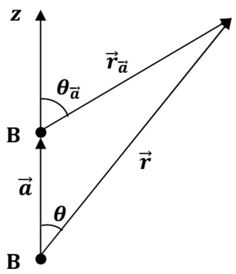
The positions of constituent atoms in diboron B₂ molecule are convenient to describe with respect to a coordinate system, the origin of which coincides with one of atoms and the $z$-axis is directed along the B–B chemical bond with length of $a$ (Figure 1).

Semi-classical single-electron Hamiltonian of this system is,

$${\widehat{H}}_{\overrightarrow{a}}(\overrightarrow{r})=-\frac{{\hslash }^2∆}{2m}+U(\overrightarrow{r})+U_{\overrightarrow{a}}(\overrightarrow{r})$$

(139)

where,

$$U(\overrightarrow{r})=U_{5 Z_{12}{Z}_{34}{Z}_5}(r)$$

(140)

and

$$U_{\overrightarrow{a}}(\overrightarrow{r})=U({\overrightarrow{r}}_{\overrightarrow{a}})$$

(141)

are the constituent boron atoms potentials and,

$${\overrightarrow{r}}_{\overrightarrow{a}}=\overrightarrow{r}-\overrightarrow{a}$$

(142)

Obviously, variable electron radius-vector $\overrightarrow{r}$ displacement by the constant vector $\overrightarrow{a}$ does not change the differential operator $∆$:

$$∆={∆}_{\overrightarrow{a}}$$

(143)

So, introducing the constituent atoms Hamiltonians,

$$\widehat{h}(\overrightarrow{r})=-\frac{{\hslash }^2∆}{2m}+U(\overrightarrow{r})$$

(144)

and

$${\widehat{h}}_{\overrightarrow{a}}(\overrightarrow{r})=-\frac{{\hslash }^2{∆}_{\overrightarrow{a}}}{2m}+U_{\overrightarrow{a}}(\overrightarrow{r})$$

(145)

we can transform the molecular Hamiltonian in two more equivalent forms:

$${\widehat{H}}_{\overrightarrow{a}}(\overrightarrow{r})=\widehat{h}(\overrightarrow{r})+U_{\overrightarrow{a}}(\overrightarrow{r})$$

(146)

and

$${\widehat{H}}_{\overrightarrow{a}}(\overrightarrow{r})={\widehat{h}}_{\overrightarrow{a}}(\overrightarrow{r})+U(\overrightarrow{r})$$

(147)

According to the law of cosines,

$$r_{\overrightarrow{a}}=\sqrt{r^2-2ar\cos \theta +a^2}$$

(148)

while according to the law of sines,

$$\frac{\sin {\theta }_{\overrightarrow{a}}}{\sin \theta }=\frac{\sin \left(\pi -{\theta }_{\overrightarrow{a}}\right)}{\sin \theta }=\frac{r}{r_{\overrightarrow{a}}}$$

(149)

and, consequently,

$$\cos {\theta }_{\overrightarrow{a}}=\frac{r\cos \theta -a}{r_{\overrightarrow{a}}}=\frac{r\cos \theta -a}{\sqrt{r^2-2ar\cos \theta +a^2}}$$

(150)

For simplicity, let us restrict ourselves with only higher valence-electron, i.e., 2p-orbitals basis in semi-classical LCAO calculations:

$$\psi (\overrightarrow{r})={\psi }_5(\overrightarrow{r})=\frac{1}{2}\sqrt{\frac{1}{2\pi }{\left(\frac{Z_5}{r_{\mathrm{B}}}\right)}^3}\left|\cos \theta \right|\left(\frac{Z_{5}r}{2r_{\mathrm{B}}}\right)\exp \left(-\frac{Z_{5}r}{2r_{\mathrm{B}}}\right)$$

(151)

and

$$\begin{gathered} {\psi }_{\overrightarrow{a}}\left(\overrightarrow{r}\right)={\psi }_5\left({\overrightarrow{r}}_{\overrightarrow{a}}\right)=\frac{1}{2}\sqrt{\frac{1}{2\pi }{\left(\frac{Z_5}{r_{\mathrm{B}}}\right)}^3}\left|\cos {\theta }_{\overrightarrow{a}}\right|\left(\frac{Z_5{r}_{\overrightarrow{a}}}{2r_{\mathrm{B}}}\right)\exp \left(-\frac{Z_5{r}_{\overrightarrow{a}}}{2r_{\mathrm{B}}}\right)= \\ =\frac{1}{2}\sqrt{\frac{1}{2\pi }{\left(\frac{Z_5}{r_{\mathrm{B}}}\right)}^3}\frac{Z_5\left|r\cos \theta -a\right|}{2r_{\mathrm{B}}}\exp \left(-\frac{Z_5\sqrt{r^2-2ar\cos \theta +a^2}}{2r_{\mathrm{B}}}\right) \end{gathered}$$

(152)

These orbitals satisfy the following eigenvalue equations,

$$\widehat{h}(\overrightarrow{r})\psi (\overrightarrow{r})=E_5\psi (\overrightarrow{r})$$

(153)

and

$${\widehat{h}}_{\overrightarrow{a}}(\overrightarrow{r}){\psi }_{\overrightarrow{a}}(\overrightarrow{r})=E_5{\psi }_{\overrightarrow{a}}(\overrightarrow{r})$$

(154)

where $E_5$ is the energy level corresponding 2p-state in boron atom:

$$\frac{E_5}{E_{\mathrm{B}}}=-\frac{Z_5^2}{4}$$

(155)

Furthermore, both orbitals are the real functions normalized according to the relations,

$${\displaystyle \int }{d}^3\overrightarrow{r}{\psi }^2(\overrightarrow{r})={\displaystyle \int }{d}^3\overrightarrow{r}{\psi }_{\overrightarrow{a}}^2(\overrightarrow{r})=1$$

(156)

In formal analogy with well-known problem of hydrogen molecular ion H₂⁺ also containing one electron and two identical sources of attractive radial electric field, we can write down energy spectrum,

$$E_a^{\pm }=\frac{C\left(a\right)\pm R\left(a\right)}{1\pm O\left(a\right)}$$

(157)

and corresponding molecular orbitals,

$${\Psi }_{\overrightarrow{a}}^{\pm }(\overrightarrow{r})=\frac{\psi (\overrightarrow{r})\pm {\psi }_{\overrightarrow{a}}(\overrightarrow{r})}{\sqrt{2(1\pm O(a))}}$$

(158)

for the electron system under consideration.

Here are introduced Coulomb, resonance and overlap integrals:

$$C\left(a\right)={\displaystyle \int }{d}^3\overrightarrow{r} \psi (\overrightarrow{r}){\widehat{H}}_{\overrightarrow{a}}(\overrightarrow{r})\psi (\overrightarrow{r})={\displaystyle \int }{d}^3\overrightarrow{r}{\psi }_{\overrightarrow{a}}(\overrightarrow{r}){\widehat{H}}_{\overrightarrow{a}}(\overrightarrow{r}){\psi }_{\overrightarrow{a}}(\overrightarrow{r})=E_5+{\displaystyle \int }{d}^3\overrightarrow{r}{\psi }_{\overrightarrow{a}}^2(\overrightarrow{r})U(\overrightarrow{r})\equiv E_5+c\left(a\right)$$

(159)

$$R\left(a\right)={\displaystyle \int }{d}^3\overrightarrow{r} \psi (\overrightarrow{r}){\widehat{H}}_{\overrightarrow{a}}(\overrightarrow{r}){\psi }_{\overrightarrow{a}}(\overrightarrow{r})=E_{5}O\left(a\right)+{\displaystyle \int }{d}^3\overrightarrow{r} \psi (\overrightarrow{r})U(\overrightarrow{r}){\psi }_{\overrightarrow{a}}(\overrightarrow{r})\equiv E_{5}O\left(a\right)+r\left(a\right)$$

(160)

$$O\left(a\right)={\displaystyle \int }{d}^3\overrightarrow{r} \psi (\overrightarrow{r}){\psi }_{\overrightarrow{a}}(\overrightarrow{r})$$

(161)

respectively.

For their complexity, the reduced Coulomb $c\left(a\right)$ and resonance $r\left(a\right)$ integrals will not be calculated here, but evaluated their combination,

$$r\left(a\right)-c\left(a\right)O\left(a\right)\approx U\left(a\right)O\left(a\right)$$

(162)

based on the constituent boron atom potential function value $U\left(a\right)$ at center of another atom.

As for the overlap integral, for new variables of integration,

$$y=\cos \theta$$

(163)

and

$$\rho =\frac{Z_{5}r}{r_{\mathrm{B}}}$$

(164)

it can is converted into the form:

$$\begin{gathered} O\left(a\right)={{\displaystyle \int }}_0^{\infty }dr r^2{{\displaystyle \int }}_0^{2\pi }d\phi {{\displaystyle \int }}_0^{\pi }d\theta \sin \theta \psi \left(\overrightarrow{r}\right){\psi }_{\overrightarrow{a}}\left(\overrightarrow{r}\right)= \\ =\frac{1}{16}{{\displaystyle \int }}_0^{\infty }d\rho {\rho }^2{{\displaystyle \int }}_{-1}^{+1}dy \left|\rho y\left(\rho y-\alpha \left(a\right)\right)\right|\exp \left(-\frac{\rho +\sqrt{{\rho }^2-2\alpha \left(a\right)\rho y+{\alpha }^2\left(a\right)}}{2}\right) \\ \approx \frac{a^2}{4r_5^2}{{\displaystyle \int }}_0^{\infty }d\rho {\rho }^2\exp \left(-\rho \right)=\frac{a^2}{2r_5^2} \end{gathered}$$

(165)

Here are introduced the designations,

$$\alpha \left(a\right)=\frac{Z_{5}a}{r_{\mathrm{B}}}$$

(166)

and

$$r_5=\frac{4r_{\mathrm{B}}}{Z_5}$$

(167)

where $r_5$ is the semi-classical radius of the 2p-orbit. In the integrand we have approximated $y~\frac{\alpha \left(a\right)}{2\rho }$ since the main contribution to the overlap integral is made by the regions of space whose points are approximately uniformly distant from the centers of atoms $r~r_{\overrightarrow{a}}$. Emphasize that obtained in this way result approximates only numerical value of the integral, not its parametric dependence.

It is expedient to convert above expression for energy levels into the form,

$$E_a^{\pm }=E_5+\frac{c\left(a\right)\pm r\left(a\right)}{1\pm O\left(a\right)}$$

(168)

yielding the energy difference,

$$\mathsf{\Delta }{E}_a^{\pm }=E_a^{-}-E_a^{+}=\frac{2\left(c\left(a\right)O\left(a\right)-r\left(a\right)\right)}{1-O^2\left(a\right)}\approx -\frac{2U\left(a\right)O\left(a\right)}{1-O^2\left(a\right)}$$

(169)

Table 3. Semi-classical parameters of diboron B₂ molecule outer shell electron states.

Orbital	a, Å	O(a)	${\mathsf{\Psi }}_{\overrightarrow{\mathit{a}}}^{\pm }$	$-\mathit{U}\left(\mathit{a}\right)$, eV	$\Delta {\mathit{E}}_{\mathit{a}}^{\pm }$, eV	${\mathit{T}}_{\mathit{e}}$, eV
Bonding	1.59	0.618	$0.556\psi (\overrightarrow{r})+0.556{\psi }_{\overrightarrow{a}}(\overrightarrow{r})$	1.82	3.64	3.79
Antibonding	1.63	0.650	$1.195\psi (\overrightarrow{r})-1.195{\psi }_{\overrightarrow{a}}(\overrightarrow{r})$	1.62	3.65

shows results of our numerical estimations together with available on diboron molecule experimental data: bond lengths $a$ in ground and lowest excited molecular states and term $T_e$ of corresponding transition [60].

Thus, semi-classically evaluated differences between electron energies in bonding and antibonding 2p-states 3.64 and 3.65 eV in diboron molecule B₂ are deviated by about 4% from experimentally obtained term of 3.79 eV. Accuracy seems to be acceptable, if take into account some simplifications utilized in addition to semi-classical approximation itself.

Underestimation of the term energy can be also related to the assumption that in process of electron transition B–B bond length remains unchanged. More detailed calculations are needed to find not only energy differences at fixed bond lengths, but also electron energy levels for both bond lengths corresponding ground and first excited states of the molecule. Then experimental term should be compared with difference between energies calculated for antibonding orbital of excited molecule and bonding orbital in its ground state.

5. Concluding Remarks

Thus, a method of semi-classical type is proposed to calculate condensed matter electronic structure.

The novelties achieved in this approach can be summarized as follows:

-

There is constructed the multi-electron atom semi-classical model, which is based on three key assumptions: (1) atomic electrons are moving in stationery self-consistent electric field; (2) intra-atomic electric field affecting electrons is spherically symmetric; and (3) atoms are semi-classical electron systems in sense of Maslov criterion, i.e., proximity of the semi-classical electron energy spectrum of atoms with exact one.

-

Electric field potential acting on atomic electron, in the vicinity of its semi-classical orbit, is approximated by Coulomb potential with effective charge number of the nucleus shielded by all other atomic electrons. Accordingly, semi-classical electron orbitals are obtained in form of effective charge number dependent hydrogen-like atomic orbitals, i.e., as analytic combination of special functions—spherical harmonics and generalized Laguerre polynomials. The set of equations determining effective charge numbers for Coulomb-like fields acting on atomic electrons is written down in explicit form.

-

On the basis of constituent atoms semi-classical electric fields, there is constructed initial approximation to the semi-classical crystal potential.

-

The LCAO method, which is looking for the condensed matter electronic subsystem wave function as a linear combination of atom-like orbitals, is formulated with semi-classical electron orbitals in constituent atoms.

-

For the LCAO secular equation determining crystal electronic structure—electron energy bands and electron density distribution in the crystal, there are found general expressions of matrix elements (overlap and electron potential energy integrals) between Bloch sums of semi-classical AOs.

Test calculations are conducted for simple electron systems such as boron atom B and diboron molecule B₂. The boron atom electronic structure is semi-classically parameterized and on the basis of this in analytical form is constructed the semi-classical potential of boron. In these specific cases, mean deviation of semi-classically evaluated electron energy levels of atomic orbitals and energy difference of molecular orbitals from corresponding atomic ionization potentials and molecular term are about a few percent.

As for the full practical realization of the introduced semi-classical method, it needs some further studies:

-

Effective nucleus charge numbers for semi-classical electron orbitals of stable neutral atoms and atomic ions in their isolated states, as well as corresponding radii of electron orbits and electron energy levels, should be computed and tabulated.

-

The semi-classical matrix elements of the secular equation should be reduced to linear combinations of a smaller number of one-, two-, and three-center overlap and potential energy integrals expressed analytically in special functions.

References

- Chkhartishvili, L. Quasi-Classical Theory of Substance Ground State; Publishing House “Technical University”: Tbilisi, Georgia, 2004. (In Russian) [Google Scholar]
- Chkhartishvili, L.S. Volume of the intersection of three spheres. Math. Notes 2001, 69, 421–428. [Google Scholar] [CrossRef]
- Chkhartishvili, L.S. Iterative solution of the secular equation. Math. Notes 2005, 77, 273–279. [Google Scholar] [CrossRef]
- Chkhartishvili, L.S. Solution of an algebraic equation using an irrational iteration function. Math. Notes 2012, 92, 714–719. [Google Scholar] [CrossRef]
- Chkhartishvili, L.; Berberashvili, T. Intra-atomic electric field radial potentials in step-like presentation. J. Electromagn. Anal. Appl. 2010, 2, 205–243. [Google Scholar] [CrossRef]
- Chkhartishvili, L.; Lezhava, D.; Tsagareishvili, O. Quasi-classical determination of electronic energies and vibration frequencies in boron compounds. J. Solid State Chem. 2000, 154, 148–152. [Google Scholar] [CrossRef]
- Chkhartishvili, L.S. Quasi-classical estimates of the lattice constant and band gap of a crystal: Two-dimensional boron nitride. Phys. Solid State 2004, 46, 2126–2133. [Google Scholar] [CrossRef]
- Chkhartishvili, L. Quasi-classical approach: Electronic structure of cubic boron nitride crystals. J. Solid State Chem. 2004, 177, 395–399. [Google Scholar] [CrossRef]
- Chkhartishvili, L. Density of electron states in wurtzite-like boron nitride: A quasi-classical calculation. Mater. Sci. Ind. J. 2006, 2, 18–23. [Google Scholar]
- Chkhartishvili, L. Zero-point vibration energy within quasi-classical approximation: Boron nitrides. Georgian e-Sci. J. Phys. 2006, 40, 130–138. [Google Scholar]
- Chkhartishvili, L.S. Analytical optimization of the lattice parameter using the binding energy calculated in the quasi-classical approximation. Phys. Solid State 2006, 48, 846–853. [Google Scholar] [CrossRef]
- Chkhartishvili, L.S. Equilibrium geometry of ultra-small radius boron nitride nanotubes. Mater. Sci. Nanostr. 2009, 1, 33–44. (In Russian) [Google Scholar]
- Chkhartishvili, L. On quasi-classical estimations of boron nanotubes ground-state parameters. J. Phys. Conf. Ser. 2009, 176, 012013. [Google Scholar] [CrossRef]
- Chkhartishvili, L.; Murusidze, I. Relative stability of BN nanotubes. Solid State Sci. 2012, 14, 1664–1668. [Google Scholar] [CrossRef]
- Chkhartishvili, L.; Murusidze, I.; Darchiashvili, M.; Tsagareishvili, O.; Gabunia, D. Metal impurities in crystallographic voids of beta-rhombohedral boron lattice: Binding energies and electron levels. Solid State Sci. 2012, 14, 1673–1682. [Google Scholar] [CrossRef]
- Chkhartishvili, L.; Murusidze, I. Frequencies of vibrations localized on interstitial metal impurities in beta-rhombohedral boron based materials. Am. J. Mater. Sci. 2014, 4, 103–110. [Google Scholar]
- Becker, R.; Chkhartishvili, L.; Avci, R.; Murusidze, I.; Tsagareishvili, O.; Maisuradze, N. “Metallic” boron nitride. Eur. Chem. Bull. 2015, 4, 8–23. [Google Scholar]
- Chkhartishvili, L. Boron quasi-planar clusters. A mini-review on diatomic approach. In Proceedings of the IEEE 7th International Conference NAP, Odessa, Ukraine, 10–15 September 2017; Pogrebnjak, A.D., Ed.; 04NESP10-1–04NESP10-5. Sumy State University: Sumy, Ukraine, 2017. [Google Scholar]
- Sartinska, L.; Chkhartishvili, L.; Voynich, E.; Eren, T.; Frolov, G.; Altay, E.; Murusidze, I.; Tsagareishvili, O.; Gabunia, D.; Maisuradze, N. Effect of concentrated light on morphology and vibrational properties of boron and tantalum mixtures. Heliyon 2018, 4, e00585. [Google Scholar] [CrossRef] [PubMed]
- Chkhartishvili, L.; Murusidze, I.; Becker, R. Electronic structure of boron flat holeless sheet. Condens. Matter 2019, 4, 28. [Google Scholar] [CrossRef]
- Chkhartishvili, L. Relative stability of planar clusters B11, B12, and B13 in neutral- and charged-states. Char. Appl. Nanomater. 2019, 2, 73–80. [Google Scholar] [CrossRef]
- Kaxiras, E. The single-particle approximation. In Atomic and Electronic Structure of Solids; Cambridge University Press: Cambridge, UK, 2010; pp. 42–81. [Google Scholar]
- Elyutin, P.V.; Krivchenkov, V.D. Quantum Mechanics with Problems; Nauka: Moscow, Russia, 1976. (In Russian) [Google Scholar]
- Jacoby, M. Introducing oganesson tetratennesside. Chem. Eng. News 2021, 99, 9. [Google Scholar] [CrossRef]
- Chkhartishvili, L. Semiclassical model of multi-electron atoms: Electronic structure calculations. In Proceedings of the Abstracts of the 5th International Conference “Nanotechnologies”, Tbilisi, Georgia, 19–22 November 2018; Gerasimov, A., Chkhartishvili, L., Chikhladze, G., Eds.; Publishing House “Technical University”: Tbilisi, Georgia, 2018; p. 36. [Google Scholar]
- Flugge, S. Practical Quantum Mechanics; Springer: Berlin/Heidelberg, Germany, 1999; Volume II. [Google Scholar]
- Morozkin, A.V.; Nirmala, R. Final element of Periodic Table is element N 137. Int. J. At. Nucl. Phys. 2020, 5, 020-1–020-4. [Google Scholar]
- Martin, B.R. Nuclear and Particle Physics; John Wiley & Sons: Chichester, UK, 2006. [Google Scholar]
- Zanzonico, P. Physics, instrumentation, and radiation safety and regulations. In Clinical Nuclear Medicine; Ahmadzadehfar, H., Biersack, H.-J., Freeman, L.M., Zuckier, L.S., Eds.; Springer Nature: Cham, Switzerland, 2020; pp. 3–48. [Google Scholar]
- Bohr, N. I. On the constitution of atoms and molecules. Phil. Mag. 1913, 26, 1–25. [Google Scholar] [CrossRef]
- Bohr, N. II. On the constitution of atoms and molecules. Phil. Mag. 1913, 26, 476–502. [Google Scholar] [CrossRef]
- Bohr, N. III. On the constitution of atoms and molecules. Phil. Mag. 1913, 26, 857–875. [Google Scholar] [CrossRef]
- Froman, N. Semi-classical and higher-order approximations: Properties, solution of connection problems. In Semi-Classical Methods in Molecular Scattering and Spectroscopy; Child, M.S., Ed.; D. Reidel Publishing Company: Dordrecht, The Netherlands, 1979; pp. 1–44. [Google Scholar]
- Hainz, J.; Grabert, H. Centrifugal terms in the WKB approximation and semi-classical quantization of hydrogen. Phys. Rev. A 1999, 60, 1698–1701. [Google Scholar] [CrossRef]
- Sergeenko, M.N. Semiclassical wave equation and exactness of the WKB method. Phys. Rev. A 1996, 53, 3798–3804. [Google Scholar] [CrossRef]
- Ghins, M. Bohr’s modeling of the atom: A reconstruction and assessment. Log. Anal. 2012, 218, 1–22. [Google Scholar]
- Potapov, A.A. Renaissance of Classical Atom; Publishing House Nauka: Moscow, Russia, 2011. (In Russian) [Google Scholar]
- Yamomoto, T.; Kaneko, K. Exploring a classical model of the helium atom. Prog. Theo. Phys. 1998, 100, 1089–1105. [Google Scholar] [CrossRef][Green Version]
- Bagchi, B.; Holody, P. An interesting application of Bohr theory. Am. J. Phys. 1988, 56, 746–747. [Google Scholar] [CrossRef]
- Tanner, G.; Richter, K.; Rost, J.-M. The theory of two-electron atoms: Between ground state and complete fragmentation. Rev. Mod. Phys. 2000, 72, 497–544. [Google Scholar] [CrossRef]
- Popa, A.-N.V. Accurate Bohr-type semi-classical model for atomic and molecular systems. Rep. Inst. Atom. Phys. 1991, E12, 1–90. [Google Scholar]
- Svidzinsky, A.A.; Scully, M.O.; Herschbach, D.R. Bohr’s 1913 molecular model revisited. Proc. Natl. Acad. Sci. USA 2005, 102, 11985–11988. [Google Scholar] [CrossRef] [PubMed]
- Thomas, L.H. The calculation of atomic fields. Proc. Camb. Phil. Soc. 1927, 23, 542–548. [Google Scholar] [CrossRef]
- Fermi, E. Un metodo statistico per la determinazione di alcune properita dell’ atomo. Atti. Accad. Naz. Lincei (Rend. Cl. Sci. Fis. Mat. Nat.) 1927, 6, 602–607. (In Italian) [Google Scholar]
- Casas, M.; Plastino, A.; Puente, A. Alternative approach to the semi-classical description of N-fermion system. Phys. Rev. A 1994, 49, 2312–2317. [Google Scholar] [CrossRef]
- Kirzhnits, D.A.; Lozovik, Y.E.; Shpatkovskaya, G.V. Statistical model of substance. Phys.—Uspekhi 1975, 117, 3–47. (In Russian) [Google Scholar]
- Magomedov, K.M. On theory of atomic quasi-classical self-consistent field. Rep. Acad. Sci. USSR 1985, 285, 1100–1115. (In Russian) [Google Scholar]
- Magomedov, K.M.; Omarova, P.M. Quasi-Classical Computing of Atomic Systems; Daghestan Scientific Centre of Russian Academy of Sciences: Makhachkala, Russia, 1989. (In Russian) [Google Scholar]
- Brack, M. The physics of simple metal clusters: Self-consistent jellium model and semi-classical approaches. Rev. Mod. Phys. 1993, 65, 677–732. [Google Scholar] [CrossRef]
- Maslov, V.P.; Fedoriuk, M.V. Semi-Classical Approximation in Quantum Mechanics; Reidel Publishing Company: Dordrecht, The Netherlands, 1981. [Google Scholar]
- Maslov, V.P. Perturbation Theory and Asymptotical Methods; Moscow State University Press: Moscow, Russia, 1965. (In Russian) [Google Scholar]
- Fischer, C.F. The Hartee–Fock Method for Atoms. A Numerical Approach; Wiley: New York, NY, USA, 1977. [Google Scholar]
- Haynes, W.M. (Ed.) CRC Handbook of Chemistry and Physics; CRC Press—Taylor & Francis Group: Boca Raton, FL, USA, 2013. [Google Scholar]
- Bassani, F.; Pastori Parravicini, G.; Ballinger, R.A. Electronic States and Optical Transitions in Solids; Franklin Book Co.: Elkins Park, PA, USA, 1993. [Google Scholar]
- Slater, J.C.; Koster, G.F. Simplified LCAO method for the periodic potential problem. Phys. Rev. 1954, 94, 1498–1524. [Google Scholar] [CrossRef]
- Halpern, V. An optimized LCAO method for crystals. J. Phys. C 1970, 3, 1900–1911. [Google Scholar] [CrossRef]
- El-Batanouny, M. Electrons and band theory: Formalism in the one-electron approximation. In Advanced Quantum Condensed Matter Physics; Cambridge University Press: Cambridge, UK, 2020; pp. 33–62. [Google Scholar]
- Prasad, R. Electronic Structure of Materials; CRC Press—Taylor & Francis Group: Boca Raton, FL, USA, 2014. [Google Scholar]
- Ma, H.; Govoni, M.; Galli, G. Quantum simulations of materials on near-term quantum computers. NPJ Comput. Mater. 2020, 6, 85. [Google Scholar] [CrossRef]
- Huber, K.-P.; Herzberg, G. Molecular Spectra and Molecular Structure, Volume 4: Constants of Diatomic Molecules; van Nostrand Reinhold Company: York, UK, 1979. [Google Scholar]
Publisher’s Note: MDPI stays neutral with regard to jurisdictional claims in published maps and institutional affiliations. |
© 2021 by the author. Licensee MDPI, Basel, Switzerland. This article is an open access article distributed under the terms and conditions of the Creative Commons Attribution (CC BY) license (https://creativecommons.org/licenses/by/4.0/).