A Quantum Model for the Dynamics of Cold Dark Matter

 , , , and
Abstract
:
1. Introduction
1.1. Classical Description of Cold Dark Matter
1.2. The Schrödinger–Poisson Model (SPM)
2. Numerical Approach
2.1. Numerical Method
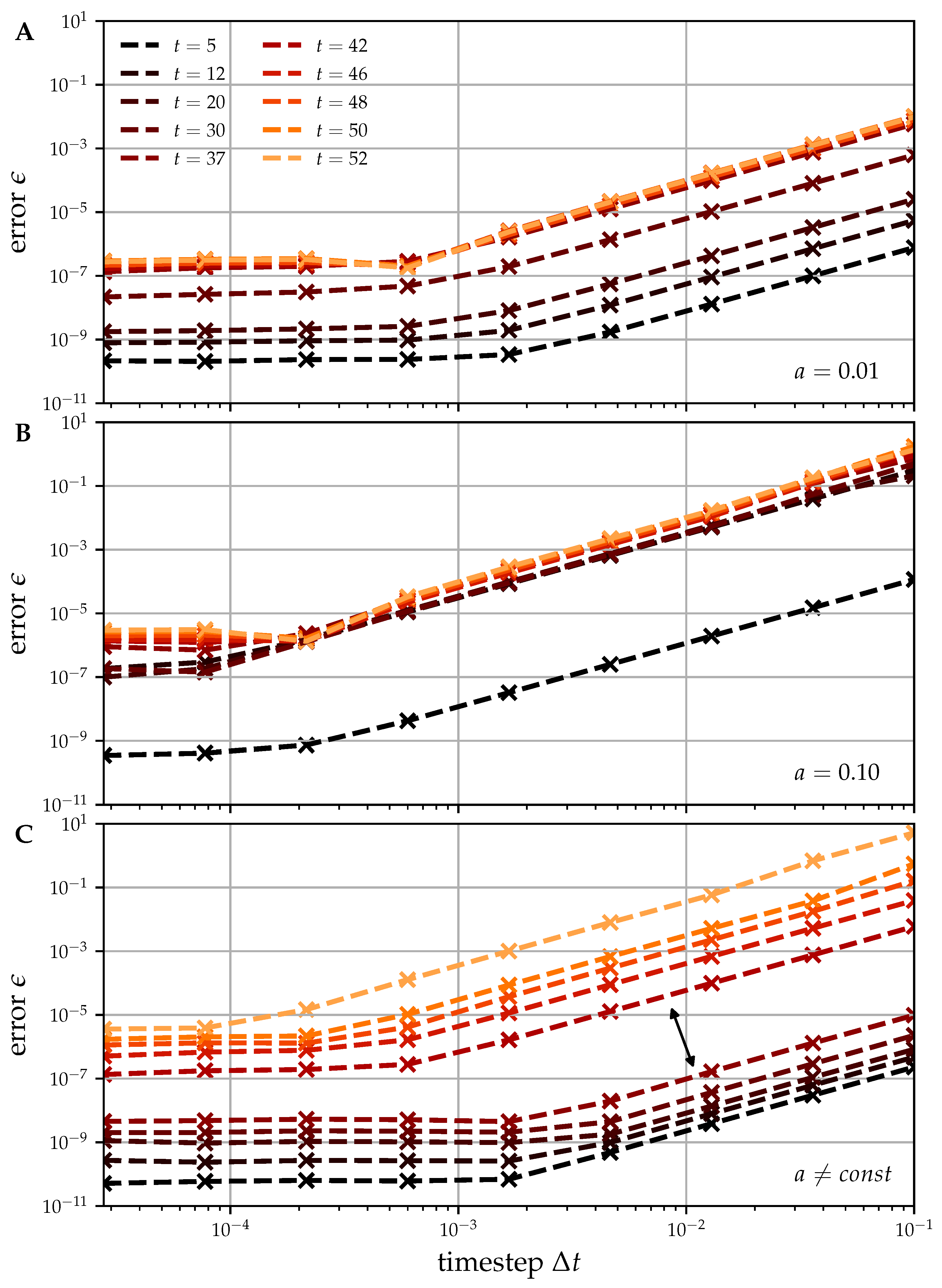
2.2. Convergence Study
3. Numerical Results
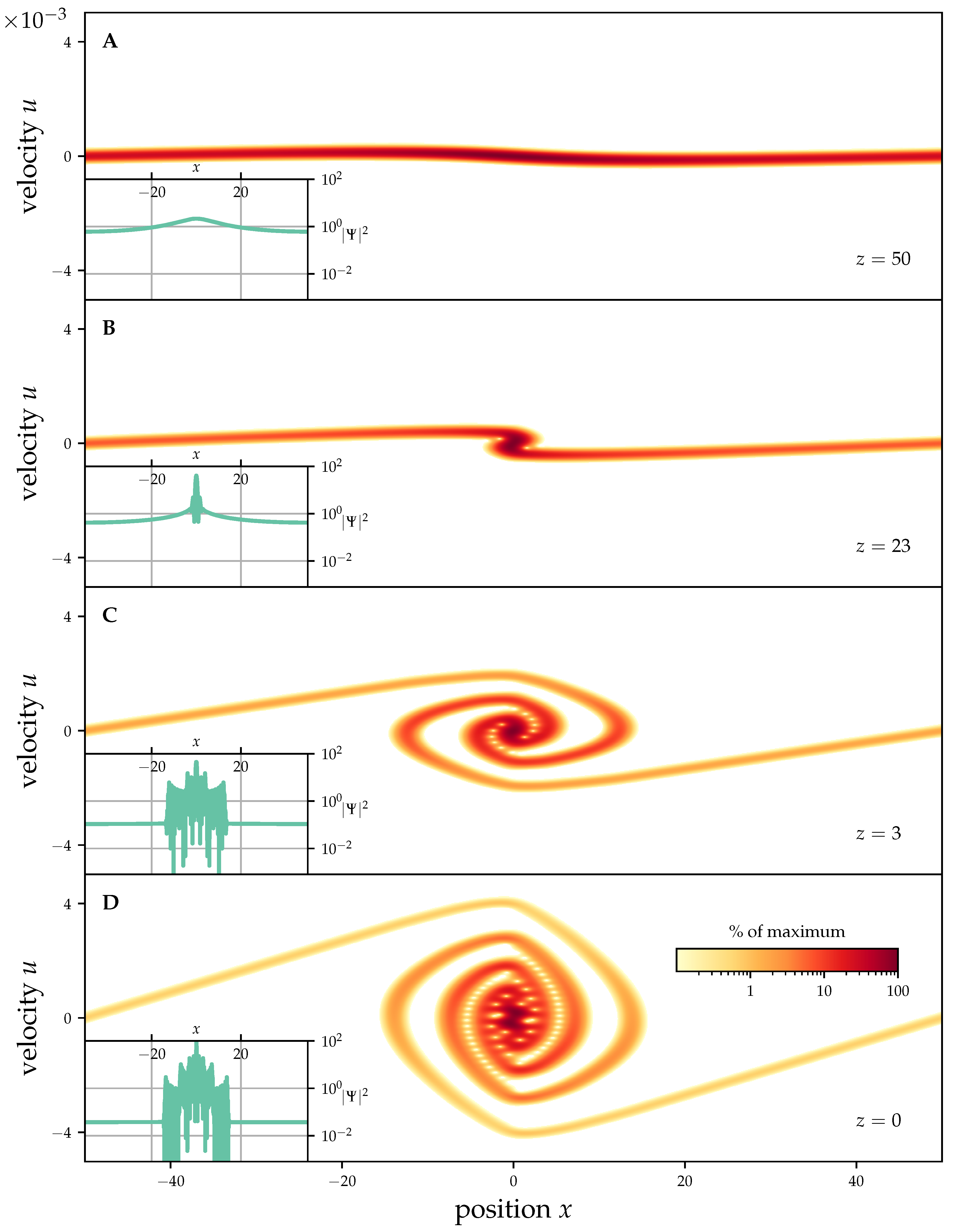
3.1. Phase Space Evolution of a Sinusoidal Perturbation
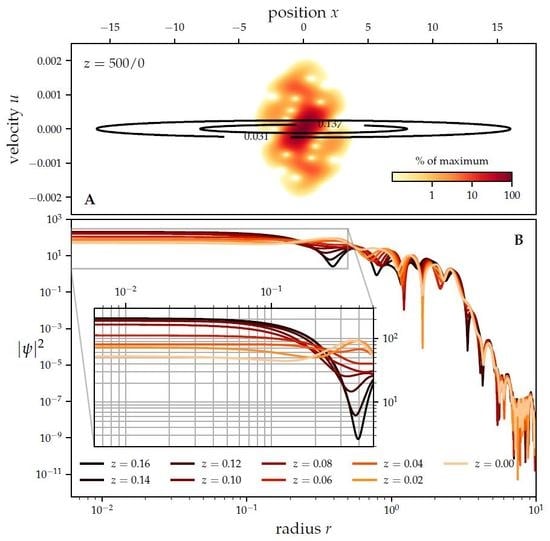
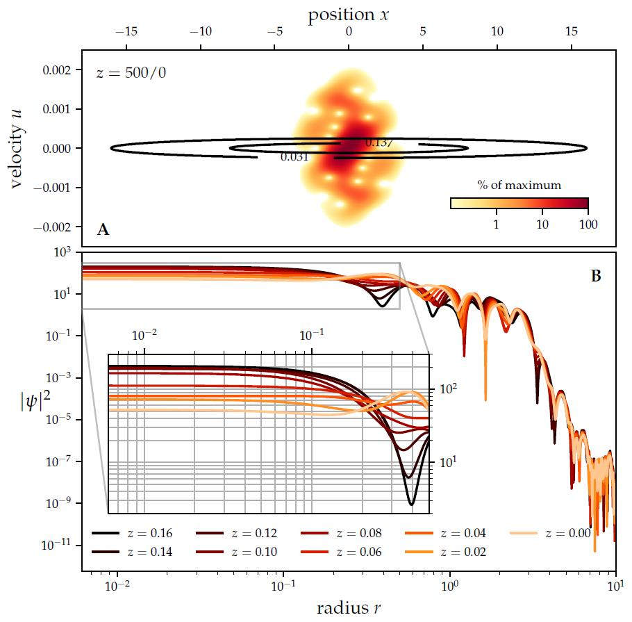
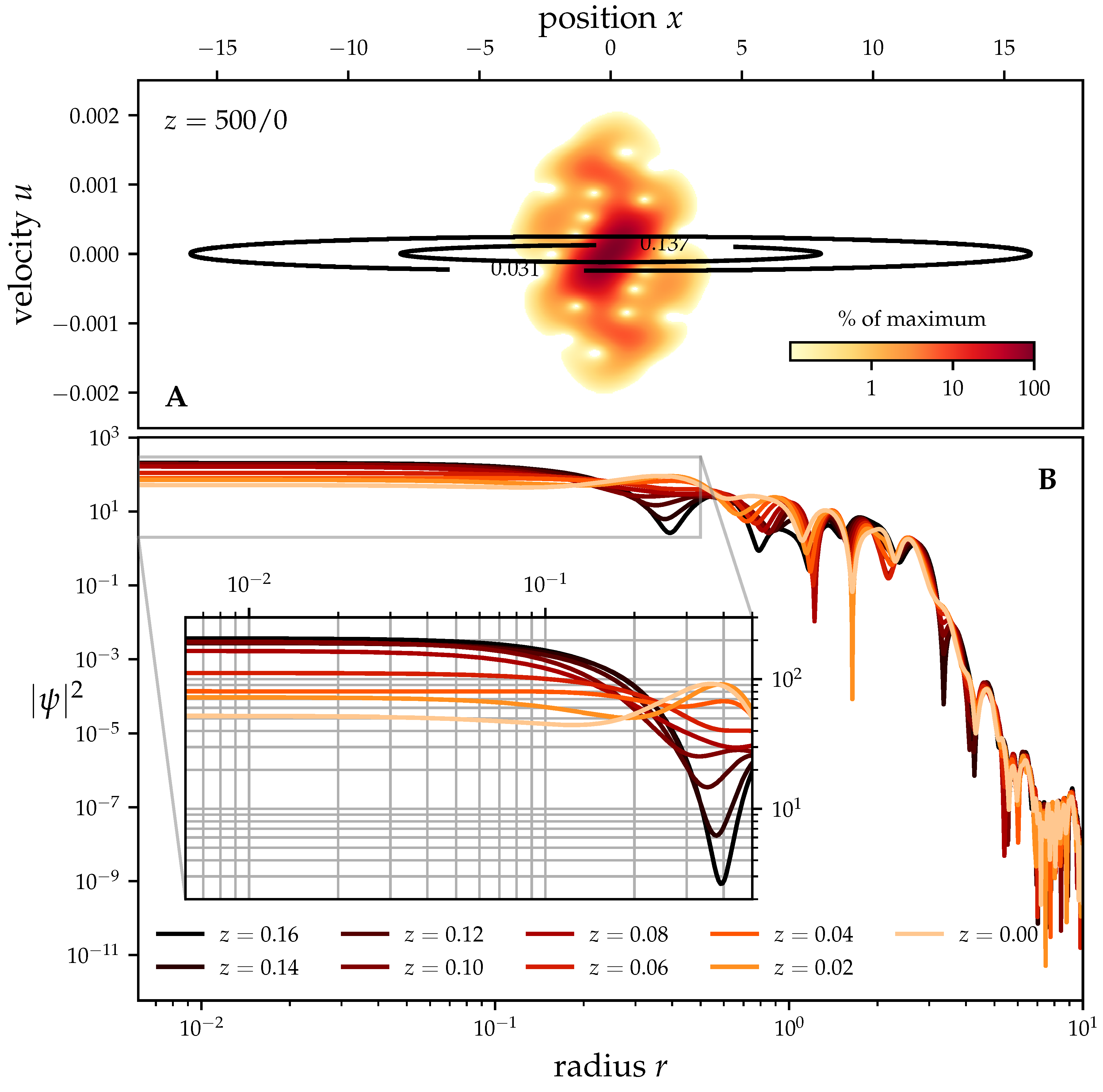
3.2. Investigation of the Dynamical Equilibrium State
3.2.1. Core Region
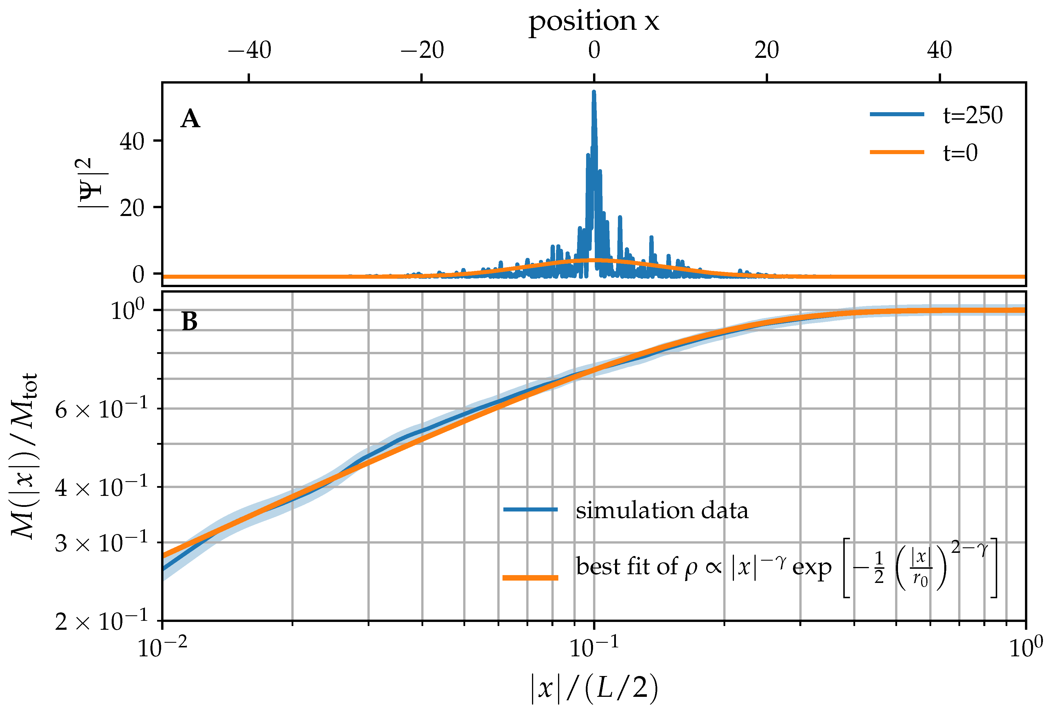
3.2.2. Halo Profile
4. Conclusions and Prospects
Author Contributions
Funding
Conflicts of Interest
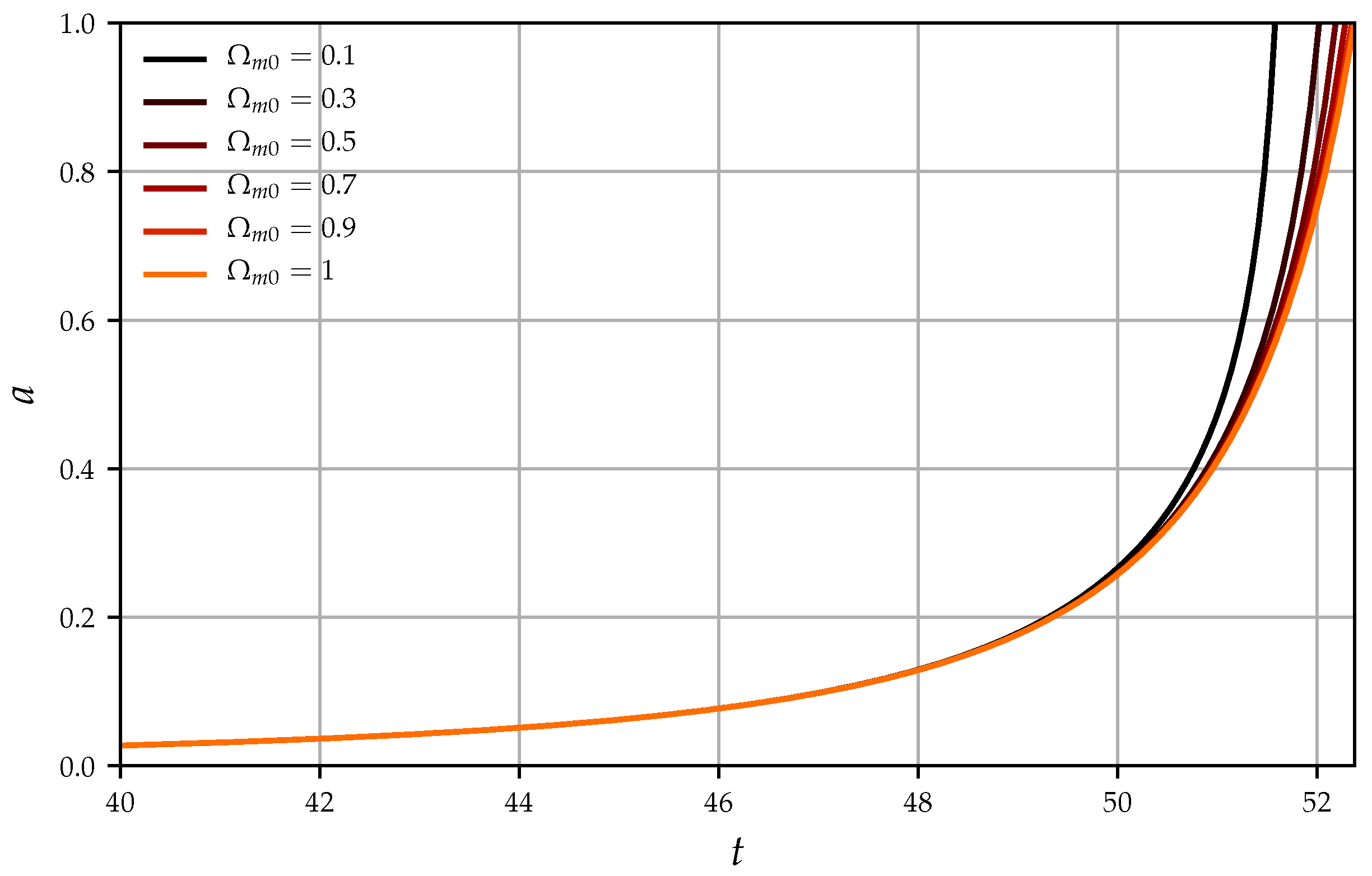
Appendix A. Cosmic Scalefactor in Code Time
References
- Boyd, R.W. Nonlinear Optics; Elsevier: Amsterdam, The Netherlands, 2008. [Google Scholar]
- Dalfovo, F.; Giorgini, S.; Pitaevskii, L.P.; Stringari, S. Theory of Bose-Einstein condensation in trapped gases. Rev. Mod. Phys. 1999, 71, 463–512. [Google Scholar] [CrossRef]
- Brian, H.; Bransden, C.J.J. Physics of Atoms and Molecules; Prentice Hall: Harlow, UK, 2003. [Google Scholar]
- Guzmán, F.S.; Ureña-López, L.A. Evolution of the Schrödinger-Newton system for a self-gravitating scalar field. Phys. Rev. D 2004, 69. [Google Scholar] [CrossRef]
- Guzman, F.S.; Urena-Lopez, L.A. Gravitational Cooling of Self-gravitating Bose Condensates. Astrophys. J. 2006, 645, 814–819. [Google Scholar] [CrossRef]
- Schive, H.Y.; Chiueh, T.; Broadhurst, T. Cosmic structure as the quantum interference of a coherent dark wave. Nat. Phys. 2014, 10, 496–499. [Google Scholar] [CrossRef]
- Schwabe, B.; Niemeyer, J.C.; Engels, J.F. Simulations of solitonic core mergers in ultralight axion dark matter cosmologies. Phys. Rev. D 2016, 94. [Google Scholar] [CrossRef]
- Mocz, P.; Vogelsberger, M.; Robles, V.H.; Zavala, J.; Boylan-Kolchin, M.; Fialkov, A.; Hernquist, L. Galaxy formation with BECDM – I. Turbulence and relaxation of idealized haloes. Mon. Not. R. Astron. Soc. 2017, 471, 4559–4570. [Google Scholar] [CrossRef]
- Peebles, P.J.E. Large-Scale Structure of the Universe; Princeton University Press: Princeton, NJ, USA, 1980. [Google Scholar]
- Collaboration, P. Planck 2018 Results. VI. Cosmological Parameters. arXiv 2019, arXiv:1807.06209v1. [Google Scholar]
- James Binney, T.S. Galactic Dynamics; Princeton University Press: Princeton, NJ, USA, 2008. [Google Scholar]
- Widrow, L.M.; Kaiser, N. Using the Schroedinger Equation to Simulate Collisionless Matter. Astrophys. J. 1993, 416, L71. [Google Scholar] [CrossRef]
- Hui, L.; Ostriker, J.P.; Tremaine, S.; Witten, E. Ultralight scalars as cosmological dark matter. Phys. Rev. D 2017, 95. [Google Scholar] [CrossRef]
- Uhlemann, C.; Kopp, M.; Haugg, T. Schrödinger method as N-body double and UV completion of dust. Phys. Rev. D 2014, 90. [Google Scholar] [CrossRef]
- Kopp, M.; Vattis, K.; Skordis, C. Solving the Vlasov equation in two spatial dimensions with the Schrödinger method. Phys. Rev. D 2017, 96. [Google Scholar] [CrossRef]
- Mocz, P.; Lancaster, L.; Fialkov, A.; Becerra, F.; Chavanis, P.H. Schrödinger-Poisson–Vlasov-Poisson correspondence. Phys. Rev. D 2018, 97. [Google Scholar] [CrossRef]
- Garny, M.; Konstandin, T. Gravitational collapse in the Schrödinger-Poisson system. J. Cosmol. Astropart. Phys. 2018, 2018, 009. [Google Scholar] [CrossRef]
- Diósi, L. Gravitation and quantum-mechanical localization of macro-objects. Phys. Lett. A 1984, 105, 199–202. [Google Scholar] [CrossRef]
- Kaminer, I.; Rotschild, C.; Manela, O.; Segev, M. Periodic solitons in nonlocal nonlinear media. Opt. Lett. 2007, 32, 3209. [Google Scholar] [CrossRef] [PubMed]
- Springel, V. The cosmological simulation code gadget-2. Mon. Not. R. Astron. Soc. 2005, 364, 1105–1134. [Google Scholar] [CrossRef]
- Springel, V.; White, S.D.M.; Jenkins, A.; Frenk, C.S.; Yoshida, N.; Gao, L.; Navarro, J.; Thacker, R.; Croton, D.; Helly, J.; et al. Simulations of the formation, evolution and clustering of galaxies and quasars. Nature 2005, 435, 629–636. [Google Scholar] [CrossRef]
- Bullock, J.S.; Boylan-Kolchin, M. Small-Scale Challenges to the ΛCDM Paradigm. Annu. Rev. Astron. Astrophys. 2017. [Google Scholar] [CrossRef]
- Schive, H.Y.; Liao, M.H.; Woo, T.P.; Wong, S.K.; Chiueh, T.; Broadhurst, T.; Hwang, W.Y.P. Understanding the Core-Halo Relation of Quantum Wave Dark Matter from 3D Simulations. Phys. Rev. Lett. 2014, 113. [Google Scholar] [CrossRef]
- Madelung, E. Quantentheorie in hydrodynamischer Form. Z. Phys. 1927, 40, 322–326. [Google Scholar] [CrossRef]
- Navarro, J.F.; Frenk, C.S.; White, S.D.M. The Structure of Cold Dark Matter Halos. Astrophys. J. 1996, 462, 563. [Google Scholar] [CrossRef]
- Flach, S.; Willis, C. Discrete breathers. Phys. Rep. 1998, 295, 181–264. [Google Scholar] [CrossRef]
- Binney, J. Discreteness effects in cosmological N-body simulations. Mon. Not. R. Astron. Soc. 2004, 350, 939–948. [Google Scholar] [CrossRef]
- Schulz, A.E.; Dehnen, W.; Jungman, G.; Tremaine, S. Gravitational collapse in one dimension. Mon. Not. R. Astron. Soc. 2013, 431, 49–62. [Google Scholar] [CrossRef]
- Sousbie, T.; Colombi, S. ColDICE: A parallel Vlasov–Poisson solver using moving adaptive simplicial tessellation. J. Comput. Phys. 2016, 321, 644–697. [Google Scholar] [CrossRef]
- Taruya, A.; Colombi, S. Post-collapse perturbation theory in 1D cosmology—beyond shell-crossing. Mon. Not. R. Astron. Soc. 2017, 470, 4858–4884. [Google Scholar] [CrossRef]
- Navarrete, A.; Paredes, A.; Salgueiro, J.R.; Michinel, H. Spatial solitons in thermo-optical media from the nonlinear Schrödinger-Poisson equation and dark-matter analogs. Phys. Rev. A 2017, 95. [Google Scholar] [CrossRef]
- Antoine, X.; Bao, W.; Besse, C. Computational methods for the dynamics of the nonlinear Schrödinger/Gross–Pitaevskii equations. Comput. Phys. Commun. 2013, 184, 2621–2633. [Google Scholar] [CrossRef]
- Lubich, C. On splitting methods for Schrödinger-Poisson and cubic nonlinear Schrödinger equations. Math. Comput. 2008, 77, 2141–2153. [Google Scholar] [CrossRef]
- Koch, O.; Neuhauser, C.; Thalhammer, M. Error analysis of high-order splitting methods for nonlinear evolutionary Schrödinger equations and application to the MCTDHF equations in electron dynamics. ESAIM Math. Model. Numer. Anal. 2013, 47, 1265–1286. [Google Scholar] [CrossRef]
- Blanes, S.; Casas, F. Splitting methods for non-autonomous separable dynamical systems. J. Phys. Math. Gen. 2006, 39, 5405–5423. [Google Scholar] [CrossRef]
- Blanes, S.; Moan, P. Practical symplectic partitioned Runge–Kutta and Runge–Kutta–Nyström methods. J. Comput. Appl. Math. 2002, 142, 313–330. [Google Scholar] [CrossRef] [Green Version]
- Blanes, S.; Casas, F.; Oteo, J.; Ros, J. The Magnus expansion and some of its applications. Phys. Rep. 2009, 470, 151–238. [Google Scholar] [CrossRef] [Green Version]
- Peebles, P.J.E. Principles of Physical Cosmology; Princeton University Press: Princeton, NJ, USA, 1993. [Google Scholar]
- Bao, W.; Jiang, S.; Tang, Q.; Zhang, Y. Computing the ground state and dynamics of the nonlinear Schrödinger equation with nonlocal interactions via the nonuniform FFT. J. Comput. Phys. 2015, 296, 72–89. [Google Scholar] [CrossRef] [Green Version]
- Woo, T.P.; Chiueh, T. High-Resolution Simulation on Structure Formation with Extremely Light Bosonic Matter. Astrophys. J. 2009, 697, 850–861. [Google Scholar] [CrossRef] [Green Version]
- LeBohec, S. Quantum Mechanical Approaches to the Virial. Available online: https://pdfs.semanticscholar.org/5d67/14575ef5d5d091cca4b01b423712f25164e9.pdf (accessed on 6 October 2019).
- Einasto, J. On the Construction of a Composite Model for the Galaxy and on the Determination of the System of Galactic Parameters. Tr. Astrofiz. Inst.-Alma-Ata 1965, 5, 87–100. [Google Scholar]
- Lev., P.; Pitaevskii, S.S. Bose-Einstein Condensation and Superfluidity; Oxford University Press: Oxford, UK, 2016. [Google Scholar]
- Kobayashi, M.; Tsubota, M. Kolmogorov Spectrum of Superfluid Turbulence: Numerical Analysis of the Gross-Pitaevskii Equation with a Small-Scale Dissipation. Phys. Rev. Lett. 2005, 94. [Google Scholar] [CrossRef] [Green Version]
- Chen, R.; Guo, H. The Chebyshev propagator for quantum systems. Comput. Phys. Commun. 1999, 119, 19–31. [Google Scholar] [CrossRef]
- Carl de Boor, C.D. A Practical Guide to Splines; Springer: Berlin/Heidelberg, Germany, 2001. [Google Scholar]


© 2019 by the authors. Licensee MDPI, Basel, Switzerland. This article is an open access article distributed under the terms and conditions of the Creative Commons Attribution (CC BY) license (http://creativecommons.org/licenses/by/4.0/).
Share and Cite
Zimmermann, T.; Pietroni, M.; Madroñero, J.; Amendola, L.; Wimberger, S. A Quantum Model for the Dynamics of Cold Dark Matter. Condens. Matter 2019, 4, 89. https://doi.org/10.3390/condmat4040089
Zimmermann T, Pietroni M, Madroñero J, Amendola L, Wimberger S. A Quantum Model for the Dynamics of Cold Dark Matter. Condensed Matter. 2019; 4(4):89. https://doi.org/10.3390/condmat4040089
Chicago/Turabian StyleZimmermann, Tim, Massimo Pietroni, Javier Madroñero, Luca Amendola, and Sandro Wimberger. 2019. "A Quantum Model for the Dynamics of Cold Dark Matter" Condensed Matter 4, no. 4: 89. https://doi.org/10.3390/condmat4040089
APA StyleZimmermann, T., Pietroni, M., Madroñero, J., Amendola, L., & Wimberger, S. (2019). A Quantum Model for the Dynamics of Cold Dark Matter. Condensed Matter, 4(4), 89. https://doi.org/10.3390/condmat4040089