Dzyaloshinskii–Moriya Coupling in 3d Insulators


Department of Theoretical Physics, Ural Federal University, 620083 Ekaterinburg, Russia
Condens. Matter 2019, 4(4), 84; https://doi.org/10.3390/condmat4040084
Submission received: 26 May 2019
/
Revised: 11 August 2019
/
Accepted: 21 September 2019
/
Published: 12 October 2019
(This article belongs to the Special Issue From cuprates to Room Temperature Superconductors)
Abstract
:We present an overview of the microscopic theory of the Dzyaloshinskii–Moriya (DM) coupling in strongly correlated 3d compounds. Most attention in the paper centers around the derivation of the Dzyaloshinskii vector, its value, orientation, and sense (sign) under different types of the (super)exchange interaction and crystal field. We consider both the Moriya mechanism of the antisymmetric interaction and novel contributions, in particular, that of spin–orbital coupling on the intermediate ligand ions. We have predicted a novel magnetic phenomenon, weak ferrimagnetism in mixed weak ferromagnets with competing signs of Dzyaloshinskii vectors. We revisit a problem of the DM coupling for a single bond in cuprates specifying the local spin–orbital contributions to the Dzyaloshinskii vector focusing on the oxygen term. We predict a novel puzzling effect of the on-site staggered spin polarization to be a result of the on-site spin–orbital coupling and the cation-ligand spin density transfer. The intermediate ligand nuclear magnetic resonance (NMR) measurements are shown to be an effective tool to inspect the effects of the DM coupling in an external magnetic field. We predict the effect of a strong oxygen-weak antiferromagnetism in edge-shared CuO chains due to uncompensated oxygen Dzyaloshinskii vectors. We revisit the effects of symmetric spin anisotropy directly induced by the DM coupling. A critical analysis will be given of different approaches to exchange-relativistic coupling based on the cluster and the DFT (density functional theory) based calculations. Theoretical results are applied to different classes of 3d compounds from conventional weak ferromagnets (-FeO, FeBO, FeF, RFeO, RCrO, …) to unconventional systems such as weak ferrimagnets (e.g., RFeCrO), helimagnets (e.g., CsCuCl), and parent cuprates (LaCuO, …).
1. Introduction
The history of the Dzyaloshinskii–Moriya interaction is closely related to the history of the discovery and investigation of weak ferromagnetism. For the first time, weak, or , ferromagnetism was observed by T. Smith [1] in 1916 in an “international family line” of natural hematite -FeO single crystalline samples from Italy, Hungary, Brasil, and Russia (Schabry, a small settlement near Ekaterinburg) and was first assigned to ferromagnetic impurities. Later the phenomenon was observed in many other 3d compounds, such as nickel fluoride NiF with rutile structure, orthorhombic orthoferrites RFeO (where R is a rare-earth element or Y), rhombohedral carbonates MnCO, NiCO, CoCO, and FeBO. However, only in 1954 L.M. Matarrese and J.W. Stout for NiF [2] and in 1956 A.S. Borovik-Romanov and M.P. Orlova for very pure synthesized carbonates MnCO and CoCO [3] have firmly established that the weak ferromagnetism is observed in chemically pure crystals with basic antiferromagnetic order and therefore it is a specific intrinsic property of some antiferromagnets. Furthermore, Borovik-Romanov and Orlova assigned the uncompensated moment in MnCO and CoCO to an overt canting of the two magnetic sublattices in an almost antiferromagnetic matrix. The model of a canted antiferromagnet became the generally adopted model of the weak ferromagnet.
A theoretical explanation and first thermodynamic theory for weak ferromagnetism in -FeO, MnCO, and CoCO was provided in 1957 by Igor Dzyaloshinskii [4,5], who wrotes the free energy of the two-sublattice uniaxial weak ferromagnet such as -FeO, MnCO, CoCO, FeBO as follows
In this expression and are unit vectors in the directions of the sublattice moments, M is the sublattice magnetization, and are basic vectors of the ferro- and antiferromagnetism, respectively, is the applied external field, is the exchange field,
is now called the Dzyaloshinskii interaction, is the Dzyaloshinskii field. The anisotropy energy is assumed to have the form: , where is the anisotropy field and the c axis is a hard direction of magnetization. Generally speaking, the Dzyaloshinskii interaction includes the terms that are linear both on ferro- and antiferromagnetic vectors. For instance, in orthorhombic orthoferrites RFeO and orthochromites RCrO the Dzyaloshinskii interaction consists both of the antisymmetric and symmetric terms
while for tetragonal fluorides NiF and CoF the Dzyaloshinskii interaction consists of the only symmetric term. The theory by Dzyaloshinskii was phenomenological one and did not clarify the microscopic nature of the Dzyaloshinskii interaction that does result in the canting. Later on, in 1960, Toru Moriya [6,7] proposed a model microscopic theory of the effective exchange-relativistic spin-spin antisymmetric interaction
now called Dzyaloshinskii–Moriya (DM) spin coupling, as a main contributing mechanism of weak ferromagnetism. Here is the axial Dzyaloshinskii vector. Presently Keffer [8] proposed a simple phenomenological expression for the Dzyaloshinskii vector for two magnetic cations M and M interacting by the superexchange mechanism via intermediate ligand O (see Figure 1):
where are unit radius vectors for O - M bonds with presumably equal bond lenghts. Later on Moskvin [9] derived a microscopic formula for the Dzyaloshinskii vector
where
with being the M-O-M superexchange bonding angle, are the O-M separations. The sign of the scalar parameter can be addressed to be the sign, or sense of the Dzyaloshinskii vector. The Formula (6) was shown to work only for the S-type magnetic ions with orbitally nondegenerate ground state, e.g., for 3d ions with half-filled shells 3d, , , (for instance, Fe, Mn, Cr, Mn, Ni).
It should be noted that sometimes instead of (6) one may use another form of the structural factor for the Dzyaloshinskii vector:
where , , l = , are radius vectors for O-M bonds, respectively.
Starting with the pioneering papers by Dzyaloshinskii [4] and Moriya [6,7] the DM coupling was extensively investigated in the 1960–80s in connection with the weak ferromagnetism focusing on hematite -FeO and orthoferrites RFeO [10,11,12,13]. Typical values of the canting angle turned out to be on the order of 0.001–0.01, in particular, in -FeO [14,15], (2.2–2.9) in LaCuO [16,17], in FeF [18], in YFeO [19], in FeBO [20]. Main exchange and DM coupling parameters for these weak ferromagnets are given in the Table 1.
Valerii Ozhogin et al. [21] in 1968 first raised the issue of the sign of the Dzyaloshinskii vector, however, the reliable local information on its sign, or to be exact, that of the Dzyaloshinskii parameter , was first extracted only in 1990 from the F ligand NMR (nuclear magnetic resonance) data in a weak ferromagnet FeF [22]. In 1977 we have shown that the Dzyaloshinskii vectors can be of opposite sign for different pairs of S-type ions [12] that allowed us to uncover a novel magnetic phenomenon, weak ferrimagnetism, and a novel class of magnetic materials, weak ferrimagnets, which are systems such as solid solutions YFeCrO with competing signs of the Dzyaloshinskii vectors and the very unusual concentration and temperature dependence of the magnetization [23,24]. The relation between Dzyaloshinskii vector and the superexchange geometry (6) allowed us to find numerically all the overt and hidden canting angles in the rare-earth orthoferrites RFeO [11] that was nicely confirmed in Fe NMR [25] and neutron diffraction [26,27,28] measurements.
The stimulus to a renewed interest to the DM coupling was given by the high-T cuprate problem, in particular, by the weak ferromagnetism observed in the parent cuprate LaCuO [16,17] and many other interesting effects for the low-dimensional DM systems, in particular, the “field-induced gap” phenomena [29,30]. At variance with typical 3d systems such as orthoferrites, the cuprates are characterized by a low-dimensionality, large diversity of Cu-O-Cu bonds including corner- and edge-sharing, different ladder configurations, strong quantum effects for the Cu centers, and a particularly strong Cu-O covalency resulting in a comparable magnitude of the hole charge/spin densities on the copper and oxygen sites. Several groups (see, e.g., refs. [31,32,33,34,35,36]) have developed the microscopic model approach by Moriya for different 1D and 2D cuprates, making use of different perturbation schemes, different types of the low-symmetry crystalline field, different approaches to the intra-atomic electron–electron correlation. However, despite a rather large number of publications and hot debates (see, e.g., refs. [37,38]) the problem of exchange-relativistic effects, that is of the DM coupling and related problem of spin anisotropy in cuprates remains to be open (see, e.g., refs. [39,40] for experimental data and discussion). Common shortcomings of current approaches to DM coupling in 3d oxides concern a problem of allocation of the Dzyaloshinskii vector and respective “weak” (anti)ferromagnetic moments, and full neglect of spin–orbital effects for “nonmagnetic” oxygen O ions, which are usually believed to play only an indirect intervening role. On the other hand, the oxygen O NMR-NQR (NQR, nuclear quadrupole resonance) studies of weak ferromagnet LaCuO [41,42] seem to evidence unconventional local oxygen “weak-ferromagnetic” polarization whose origin cannot be explained in frames of current models.
In recent years interest has shifted towards other manifestation of the DM coupling, such as the magnetoelectric effect [43,44], so-called flexoelectric effect in multiferroic bismuth ferrite with coexisting spin canting and the spin cycloidal ordering [45], and skyrmion states [46], where reliable theoretical predictions have been lacking.
Phenomenologically antisymmetric DM coupling in a continual approximation gives rise to the so-called Lifshitz invariants, or energy contributions linear in first spatial derivatives of the magnetization [47]
where is a spatial coordinate. These chiral interactions derived from the DM coupling stabilize localized (vortices) and spatially modulated structures with a fixed rotation sense of the magnetization [46]. In fact, these are believed to be the only mechanisms to induce nanosize skyrmion structures in condensed matter.
In this paper we present an overview of the microscopic theory of the DM coupling in strongly correlated compounds such as 3d oxides. The rest part of the paper is organized as follows. In Section 2 we shortly address main results of the microscopic theory of the isotropic superexchange interactions for so-called S-type ions focusing on the angular dependence of the exchange integrals. Most attention in Section 3 centers around the derivation of the Dzyaloshinskii vector, its value, orientation, and sense (sign) under different types of the (super)exchange interaction and crystal field. Theoretical predictions of this section are compared in Section 4 with experimental data for the overt and hidden canting in orthoferrites. Here, too, we consider a weak ferrimagnetism, a novel type of magnetic ordering in systems with competing signs of the Dzyaloshinskii vectors. The ligand NMR in weak ferromagnet FeF and the first reliable determination of the sign of the Dzyaloshinskii vector are considered in Section 5. An alternative method to derive DM coupling is discussed in Section 6 by the example of the three-center two-electron/hole system such as a triad Cu-O-Cu in cuprates. Here we emphasize specific features of the ligand contribution to the DM coupling and some inconsistencies of its traditional form. As a direct application of the theory, we address in Section 7 the O NMR in LaCuO and argue that the field-induced staggered magnetization due to DM coupling does explain a puzzling Knight shift anomaly. In Section 8 we consider features of the DM coupling in helimagnetic cuprate CsCuCl. Short Section 9 is devoted to puzzling features of the exchange-relativistic two-ion symmetric spin anisotropy due to DM coupling in quantum s = 1/2 magnets. So-called “first-principles” calculations of the exchange interactions and DM coupling are critically discussed in Section 10. A short summary is presented in Section 11.
2. Microscopic Theory of the Isotropic Superexchange Coupling
DM coupling is derived from the off-diagonal (super)exchange coupling and does usually accompany a conventional (diagonal) Heisenberg type isotropic (super)exchange coupling:
The modern microscopic theory of the (super)exchange coupling had been elaborated by many physicists starting with well-known papers by P. Anderson [48,49], especially intensively in 1960–70s (see review article [50]). Numerous papers devoted to the problem pointed to the existence of many hardly estimated exchange mechanisms, seemingly comparable in value, in particular, for superexchange via intermediate ligand ion to be the most interesting for strongly correlated systems such as 3d oxides. Unfortunately, up to now, we have no reliable estimations of the exchange parameters, though on the other hand we have no reliable experimental information about their magnitudes. To that end, many efforts were focused on the fundamental points such as many-electron theory and orbital dependence [9,51,52,53,54], crystal-field effects [55], off-diagonal exchange [56], exchange in excited states [57], the angular dependence of the superexchange coupling [9]. The irreducible tensor operators (the Racah algebra) were shown to be a very instructive tool both for description and analysis of the exchange coupling in the 3d- and 4f-systems [9,51,52,53,54,55].
First poor man’s microscopic derivation for the dependence of the superexchange integral on the bonding angle (see Figure 1) was performed by the author in 1970 [9] under simplified assumptions. As a result, for S-ions with configuration 3d (Fe, Mn)
where parameters depend on the cation-ligand separation. A more comprehensive analysis has supported the validity of the expression. Interestingly, the second term in (11) is determined by the ligand inter-configurational - excitations, while other terms are related with intra-configurational -, -contributions.
Later on, the derivation had been generalized for the ions in a strong cubic crystal field [13]. Orbitally isotropic contribution to the exchange integral for pair of 3d-ions with configurations can be written as follows
where are effective “g-factors” of the subshells of ion 1 and 2, respectively:
Kinetic exchange contribution to partial exchange parameters related with the electron transfer to partially filled shells can be written as follows [13,55]
where are positive definite d-d transfer integrals, U is a mean d-d transfer energy (correlation energy). All the partial exchange integrals appear to be positive or “antiferromagnetic”, irrespective of the bonding angle value, though the combined effect of the and bonds in yields a ferromagnetic contribution given bonding angles . It should be noted that the “large” ferromagnetic potential contribution [58] has a similar angular dependence [57].
Some predictions regarding the relative magnitude of the exchange parameters can be made using the relation among different d-d transfer integrals as follows
where are covalency parameters. The simplified kinetic exchange contribution (14) related with the electron transfer to partially filled shells does not account for intra-center correlations which are of a particular importance for the contribution related with the electron transfer to empty shells. For instance, appropriate contributions related with the transfer to empty subshell for the Cr-Cr and Fe-Cr exchange integrals are
where is the energy separation between and terms for configuration (Cr ion). Obviously, these contributions have a ferromagnetic sign. Furthermore, the exchange integral I(CrCr) can change sign at = :
Microscopically derived angular dependence of the superexchange integrals does nicely describe the experimental data for exchange integrals I(FeFe), I(CrCr), and I(FeCr) in orthoferrites, orthochromites, and orthoferrites-orthochromites [59] (see Figure 2). The fitting allows us to predict the sign change for I(CrCr) and I(FeCr) at ≈ 133 and 170, respectively. In other words, the Cr-O-Cr (Fe-O-Cr) superexchange coupling becomes ferromagnetic at (). However, it should be noted that too narrow (141–156) range of the superexchange bonding angles we used for the fitting with assumption of the same Fe(Cr)-O bond separations and mean superexchange bonding angles for all the systems gives rise to a sizeable parameter’s uncertainty, in particular, for I(FeFe) and I(FeCr). In addition, it is necessary to note a large uncertainty regarding what is here called the “experimental” value of the exchange integral. The fact is that the “experimental” exchange integrals we have just used above are calculated using simple MFA relation
however, this relation yields the exchange integrals that can be one and a half or even twice less than the values obtained by other methods [13,60].
Above, we addressed only typically antiferromagnetic kinetic (super)exchange contribution as a result of the second order perturbation theory. However, actually this contribution does compete with typically ferromagnetic potential (super)exchange contribution, or Heisenberg exchange, which is a result of the first order perturbation theory. The most important contribution to the potential superexchange can be related with the intra-atomic ferromagnetic Hund exchange interaction of unpaired electrons on orthogonal ligand orbitals hybridized with the d-orbitals of the two nearest magnetic cations.
Strong dependence of the superexchange integrals on the cation-ligand-cation separation is usually described by the Bloch’s rule [61]:
3. Microscopic Theory of the DM Coupling
3.1. Moriya’s Microscopic Theory
First microscopic theory of weak ferromagnetism, or theory of anisotropic superexchange interaction was provided by Moriya [6,7], who extended the Anderson theory of superexchange to include spin–orbital coupling . Moriya started with the one-electron Hamiltonian for d-electrons as follows
where
is a spin–orbital correction to transfer integral, m and are orbitally nondegenerate ground states on sites f and , respectively. Then Moriya did calculate the generalized Anderson kinetic exchange that contains both conventional isotropic exchange and anisotropic symmetric and antisymmetric terms, that is quasidipole anisotropy and DM coupling, respectively. We emphasize that the expression for the Dzyaloshinskii vector
has been obtained by Moriya assuming orbitally nondegenerate ground states m and on sites f and , respectively. It is worth noting that the spin-operator form of the DM coupling follows from the relation:
which is a simple consequence of the spin algebra, in particular, of the commutation relations for the spin projection operators.
Moriya found the symmetry constraints on the orientation of the Dzyaloshinskii vector . Let two ions 1 and 2 are located at the points A and B, respectively, with C point bisecting the AB line:
- When C is a center of inversion: .
- When a mirror plane ⊥AB passes through C, mirror plane or AB.
- When there is a mirror plane including A and B, mirror plane.
- When a twofold rotation axis ⊥ AB passes through C, twofold axis.
- When there is an n-fold axis (n ≥ 2) along AB, AB.
Despite its seeming simplicity the operator form of the DM coupling (4) raises some questions and doubts. First, at variance with the scalar product the vector product of the spin operators changes the spin multiplicity, that is the net spin , that underscores the need for quantum description. Spin nondiagonality of the DM coupling implies very unusual features of the -vector somewhat resembling vector orbital operator whose transformational properties cannot be isolated from the lattice [62]. It seems the -vector does not transform as a vector at all.
Another issue that causes some concern is the structure and location of the vector and corresponding spin cantings. Obviously, the vector should be related in one or another way to spin–orbital contributions localized on sites 1 and 2, respectively. These components may differ in their magnitude and direction, while the operator form (4) implies some averaging both for vector and spin canting between the two sites.
Moriya did not take into account the effects of the crystal field symmetry and strength and did not specify the character of the (super)exchange coupling, that, as we will see below, can crucially affect the direction and value of the Dzyaloshinskii vector up to its vanishing. Furthermore, he made use of a very simplified form (21) of the spin–orbital perturbation correction to the transfer integral (see Exp. (2.5) in ref. [6,7]). The fact is that the structure of the charge transfer matrix elements implies the involvement of several different on-site configurations (). Hence, the perturbation correction has to be more complicated than (21), at least, it should involve the spin–orbital matrix elements (and excitation energies!) for one- and two-particle configurations. As a result, it does invalidate the author’s conclusion about the equivalence of the two perturbation schemes, based on the corrections to the transfer integral and to the exchange coupling, respectively. Another limitation of the Moriya’s theory is related to the full neglect of the ligand spin–orbital contribution to DM coupling. Despite these shortcomings the Moriya’s estimation for the ratio between the magnitudes of the Dzyaloshinskii vector and isotropic exchange J: , where g is the gyromagnetic ratio, is its deviation from the free-electron value, respectively, in some cases may be helpful, however, only for a very rough estimation.
3.2. Microscopic Theory of the DM Coupling: Direct Exchange Interaction of the S-Type Ions
We start with a derivation of the DM coupling in the pair of the exchange coupled free ions with valent and shells to be a result of the second-order perturbation theory as a combined effect of the exchange and spin–orbital couplings when schematically
where excited states are the terms which are allowable one by the spin–orbital selection rules , . Spin–orbit interaction has a fairly simple form , whereas for the exchange interaction Hamiltonian one has to use a complex expression in terms of irreducible tensor operators [9,12,51,52,53,54,63]. The task seems to be more limited to academic interest, however, it is of a great importance from methodological point of view. After some routine though rather intricate procedure we arrive at the Dzyaloshinskii vector to be a complicated “multistory” irreducible orbital operator as follows [12]
where we make use of standard notations for -symbols, irreducible matrix elements, spectroscopic coefficients, and irreducible tensor products [63,64,65,66]. Matrix elements of irreducible tensor operators are defined by the Wigner–Eckart theorem [64,65] as follows
For the exchange parameters we have a simple dependence on the pair radius-vector: , where is the tensor spherical harmonics (). Here in (25) we took into account while the contribution of has the same expression with the minus sign and the 1↔2 permutation. In addition, we restrict ourselves by the DM coupling operator which is diagonal on the spin and orbital moments. Obviously, nonzero DM coupling is only at even value of () and . In addition () should also be an even number. Thus we should conclude that for the pair of equivalent free S-ions (Fe, Mn) when = 0 we have no DM coupling [13]. We arrive at the same conclusion, if to take into account that the exchange parameters and specifying the appropriate contribution turn into zero [13]. The appearance of the DM coupling in such a case can be driven by the inter-configurational or crystal field effects.
As the most illustrative example we consider a pair of 3d ions such as Fe, or Mn with the ground state in an intermediate octahedral crystal field which does split the terms into crystal terms and mix the crystal terms with the same octahedral symmetry, that is with the same ’s [67]. Spin–orbital coupling does mix the ground state with the term, however the term has been mixed with other terms, and . Namely the latter effect is believed to be a decisive factor for appearance of the DM coupling. The wave functions can be easily calculated by a standard technique [67] as follows [13]:
given the crystal field and intra-atomic correlation parameters [67] typical for orthoferrites [68]: 10Dq = 12,200 cm; B = 700 cm; C = 2600 cm.
The huge expression (25) reduces to a more compact form as follows:
where is the conventional spectroscopic Racah coefficient [64], , are the mixing coefficients for the term, are the -symmetry combinations of the exchange parameters. It is worth noting the conclusive effect of the - mixing.
For the direct exchange we have a simple expression for the parameters
where is the -symmetry combination, or cubic harmonics. Finally we arrive at a remarkable relation:
where the -symmetry combinations of spherical harmonics are taken in local coordinate systems for the first and second ions, respectively, and are determined by the spin–orbital coupling on the sites 1 and 2, respectively. For locally equivalent Fe3+ centers and . In the coordinate axes with
and
where and are polar and azimuthal angles of the vector. Obviously, the Dzyaloshinskii vector turns into zero, if local crystal field axes coincide for the both ions. In addition, = 0, if , that is to any symmetry axis for the first and second site. If lies in a mirror plane ⊥ mirror plane. It should be pointed out a very untypical vector character of the Dzyaloshinskii vector.
3.3. Microscopic Theory of the DM Coupling: Superexchange Interaction of the S-Ions
Hamiltonian for the superexchange coupling of two ions with electron configurations and via intermediate nonmagnetic ligand ion has the same general expression as for direct exchange [13], however, with a specific dependence of the exchange parameters on the superexchange geometry:
In the local coordinate system for the site 1 with we can write out the superexchange parameter as follows
where is the Clebsch–Gordan coefficient [64,65]. Obviously, for the superexchange mechanisms related with a particular ligand or electrons we have for : or , respectively. For mechanisms related with the ligand inter-configurational excitations . Taking into account the properties of the coefficients (30) we see that since it follows that the terms with and in (33) can be expressed in terms of the vector product = . Indeed
Obviously, final expression for the Dzyaloshinskii vector can be written as follows
with
where the first and the second terms are determined by the superexchange mechanisms related with the ligand inter-configurational excitations and intra-configurational effects, respectively. It should be noted that given = , where , the Dzyaloshinskii vector changes its sign.
3.4. Microscopic Theory of the DM Coupling: Superexchange Interaction of the S-Type Ions in a Strong Cubic Crystal Field
Hereafter we address the DM coupling for the S-type magnetic 3d ions with orbitally nondegenerate high-spin ground state in a strong cubic crystal field, that is for the 3d ions with half-filled shells , , and ground states , , , respectively. The strong crystal field approximation seems to be more appropriate for the most part of 3d ions in crystals. In particular, for the terms of the 3d ion in a strong cubic crystal field approximation instead of expressions (26) we arrive at a superposition of the wave functions for different configurations ( = 5) [67]. Using the same crystal field and correlation parameters as in expressions (26) we get a triplet of new functions as follows
with a more clearly defined contribution of a particular configuration compared with the intermediate crystal field scheme.
Making use of expressions for spin–orbital coupling [63] and main kinetic contribution to the superexchange parameters, that define the DM coupling, after routine algebra we have found that the DM coupling can be written in a standard form (36), where can be written as follows [12,13]
where the X and Y factors do reflect the exchange-relativistic structure of the second-order perturbation theory and details of the electron configuration for S-type ion. The exchange factors X are
where , are effective g-factors for , subshells, respectively, are positive definite d - d transfer integrals, U is the d - d transfer energy (correlation energy). The dimensionless factors Y are determined by the spin–orbital constants and excitation energies as follows
where are spectroscopic coefficients for cubic point group [63] and summation runs on all the terms , mixed by the spin–orbital coupling with the ground state term (, ). It should be noted that the nonzero DM coupling for S-type ions can be obtained only due to inter-configurational interaction. The factors X and Y are presented in Table 2 for S-type 3d-ions. There is the spin–orbital parameter, is the energy of the crystal term.
The signs for X and Y factors in Table 2 are predicted for rather large superexchange bonding angles which are typical for many 3d compounds such as oxides and a relation which is typical for high-spin configurations.
It is worth noting that while working with the paper we have detected and corrected a casual and unintentional error in sign of the parameters having made both in our earlier papers [12,13] and very recent paper ref. [69]. Hereafter we present correct signs for in (40) and Table 2.
Rather simple expressions (40) and (41) for the factors and do not take into account the mixing/interaction effects for the terms with the same symmetry and the contribution of empty subshells to the exchange coupling (see ref. [13]). Nevertheless, the data in Table 2 allow us to evaluate both the numerical value and sign of the parameters.
It should be noted that for critical angle , when the Dzyaloshinskii vector changes its sign we have for pairs and for pairs. Making use of different experimental data for covalency parameters (see, e.g., ref. [70]) we arrive at and for pairs in oxides.
Relation among different X’s given the superexchange geometry and covalency parameters typical for orthoferrites and orthochromites [13] is
however, it should be underlined its sensitivity both to superexchange geometry and covalency parameters. Simple comparison of the exchange parameters X (see (40) and Table 2) with exchange parameters (14) evidences their close magnitudes. Furthermore, the relation (15) allows us to maintain more definite correspondence.
Given typical values of the cubic crystal field parameter 1.5 eV we arrive at a relation among different Y’s [13]
with , , .
The highest value of the factor is predicted for pairs, while for pairs one expects a much less (may be one order of magnitude) value. The factor for pairs is predicted to be somewhat above the value for pairs. For different pairs: ; ; . Puzzlingly, that despite strong isotropic exchange coupling for and pairs, the DM coupling for these pairs is expected to be the least one among the S-type pairs. For pairs, in particular, Fe-Fe we have two compensation effects. First, the -bonding contribution to the X parameter is partially compensated by the -bonding contribution, second, the contribution of the term of the configuration is partially compensated by the contribution of the term of the configuration.
Theoretical predictions of the corrected sign of the Dzyaloshinskii vector in pairs of the S-type 3d-ions with local octahedral symmetry (the sign rules) are presented in Table 3. The signs for , , and pairs turn out to be the same but opposite to signs for and pairs. In a similar way to how different signs of the conventional exchange integral determine different (ferro-antiferro) magnetic orders the different signs of the Dzyaloshinskii vectors create a possibility of nonuniform (ferro-antiferro) ordering of local weak (anti)ferromagnetic moments, or local overt/hidden cantings. Novel magnetic phenomenon and novel class of magnetic materials, which are systems such as solid solutions YFeCrO with competing signs of the Dzyaloshinskii vectors will be addressed below (Section 4.3) in more detail.
3.5. DM Coupling in Trigonal Hematite -
Making use of our theory based on the bare ideal octahedral symmetry of S-type ions to the classical weak ferromagnet -FeO we arrive at a little unexpected disappointment, as the theory does predict that the contribution of the three equivalent Fe-O-Fe superexchange pathes for the two corner shared FeO octahedrons to the net Dzyaloshinskii vector strictly turns into zero. Exactly the same result will be obtained, if we consider the direct Fe-Fe exchange in the system of two ideal FeO octahedrons bonded through the three common oxygen ions when . Obviously, it is precisely this fact that caused a tiny spin canting in hematite being an order of magnitude smaller than, e.g., in orthoferrites RFeO or borate FeBO. So what was the real reason of weak ferromagnetism in -FeO as “opening a new page of weak ferromagnetism”? What is a microscopic origin of nonzero Dzyaloshinskii vector which should be directed along the symmetry axis according Moriya rules? First of all we should consider trigonal distortions for the octahedrons which have a symmetry and give rise to a mixing of the terms with and terms. The best way to solve the problem in principle is to proceed with a coordinate system where axis is directed along the symmetry axis rather than with the usually applied geometry.
In the coordinate axes with the nonzero coefficients have another expression [71]. Instead of (30) we arrive at
It is easy to see that for , that means that all the components of the two contributions to Dzyaloshinskii vector (29) turn into zero.
However, the situation changes under axial (trigonal) distortion of the FeO octahedrons that can be described by a simple effective Hamiltonian as follows
where () is the only irreducible tensor operator permitted by the symmetry of the distortion, is a trigonal field parameter. Such a distortion gives rise to a mixing of the terms with , , and terms. As a result the bare functions are transformed as follows:
where is a normalization coefficient, , are the mixing coefficients. The Dzyaloshinskii vector now has a representation as follows
where we again suggest the possibility of nonequivalent centers 1,2. Cubic harmonics one can find, if make use of data from ref. [71]
We see that given the only nonzero cubic harmonic is that defines the only nonzero z-component of Dzyaloshinskii vector as for only . Thus the axial distortion along the Fe-Fe bond can induce the DM coupling with Dzyaloshinskii vector directed along the bond, however, only for locally nonequivalent Fe centers, otherwise we arrive at an exact compensation of the contributions of the spin–orbital couplings on sites 1 and 2.
Trigonal hematite -FeO has the same crystal symmetry as weak ferromagnet FeBO. Furthermore, the borate can be transformed into hematite by the Fe ion substitution for B with a displacement of both “old” and “new” iron ions along trigonal axis. As a result we arrive at emergence of an additional strong isotropic (super)exchange coupling of three-corner-shared non-centrosymmetric FeO octahedra with short Fe-O separations (1.942 Å) that determines very high Néel temperature = 948 K in hematite as compared with = 348 K in borate. However, the symmetry of these exchange bonds points to a distinct compensation of the two Fe-ion’s contribution to Dzyaloshinskii vector. In other words, weak ferromagnetism in hematite -FeO is determined by the DM coupling for the same Fe-O-Fe bonds as in borate FeBO. However, the Fe-O separations for these bonds in hematite (2.111 Å) are markedly longer than in borate (2.028 Å) that points to a significantly weaker DM coupling. Combination of weaker DM coupling and stronger isotropic exchange in -FeO as compared with FeBO does explain the one order of magnitude difference in canting angles.
3.6. DM Coupling with Participation of Rare-Earth Ions
Spin–orbital interaction for the rare-earth ions with valent configuration is diagonalized within the multiplets hence the conventional DM coupling
( are the Lande factors) can arise for superexchange only due to a spin–orbital contribution on intermediate ligands. Obviously, for the rare-earth-3d-ion (super)exchange we have an additional contribution of the 3d-ion spin–orbital interaction. The rare-earth-3d-ion DM coupling Gd-O-Fe
has been theoretically and experimentally considered in ref. [72] for GdFeO.
4. Theoretical Predictions as Compared with Experiment
4.1. Overt and Hidden Canting in Orthoferrites
At variance with isotropic superexchange coupling the DM coupling has a much more complicated structural dependence. In Table 4 we present structural factors for the superexchange coupled Fe-O-Fe pairs in orthoferrites with numerical values for YFeO [73]. In all cases, the vector is oriented to the Fe ion in the position (1/2,0,0), the vectors are oriented to the nearest Fe ions in the -plane (1a, 1b) or along the c-axis (3a). It is easy to see that the weak ferromagnetism in orthoferrites governed by the y-component of the
In 1975 we made use of simple formula for the Dzyaloshinskii vector (6) and structural factors from Table 4 to find a relation between crystallographic and canted magnetic structures for four-sublattice’s orthoferrites RFeO and orthochromites RCrO [11,13] (see Figure 3), where main G-type antiferromagnetic order is accompanied by both overt canting characterized by ferromagnetic vector (weak ferromagnetism!) and two types of a hidden canting, and (weak antiferromagnetism!):
where are unit cell parameters, are oxygen () parameters [73], l is a mean cation-anion separation. These relations imply an averaging on the Fe-O-Fe bonds in plane and along c-axis. It is worth noting that .
First of all we arrive at a simple relation between crystallographic parameters and magnetic moment of the Fe-sublattice: in units of G · g/cm
where and V are the unit cell density and volume, respectively. The overt canting can be calculated through the ratio of the Dzyaloshinskii () and exchange () fields as follows
If we know the Dzyaloshinskii field we can calculate the parameter in orthoferrites as follows
that yields 3.2 K in YFeO given = 140 kOe [19]. It is worth noting that despite 0.01 the parameter is only one order of magnitude smaller than the exchange integral in YFeO.
Our results have stimulated experimental studies of the hidden canting, or “weak antiferromagnetism” in orthoferrites. As shown in Table 5 theoretically predicted relations between overt and hidden canting nicely agree with the experimental data obtained for different orthoferrites by NMR [25] and neutron diffraction [26,27,28,74].
4.2. The DM Coupling and Effective Magnetic Anisotropy
Hereafter we demonstrate a contribution of the DM coupling into effective magnetic anisotropy in orthoferrites. The classical energies of the three spin configurations in orthoferrites , , and given , , can be written as follows [75]
with obvious relation . The energies allow us to find the constants of the in-plane magnetic anisotropy (, planes), ( plane): ; ; . Detailed analysis of different mechanisms of the magnetic anisotropy of the orthoferrites [75] points to a leading contribution of the DM coupling. Indeed, for all the orthoferrites RFeO (R = Y, or rare-earth ion) this mechanism does predict a minimal energy for configuration which is actually realized as a ground state for all the orthoferrites, if one neglects the R-Fe interaction. Furthermore, predicted value of the constant of the magnetic anisotropy in -plane for YFeO = 2.0 erg/cm is close enough to experimental value of 2.5 erg/cm [19]. Interestingly, the model predicts a close energy for and configurations so that is about one order of magnitude less than and for most orthoferrites [75]. It means the anisotropy in -plane will be determined by a competition of the DM coupling with relatively weak contributors such as magneto-dipole interaction and single-ion anisotropy. It should be noted that the sign and value of the is of a great importance for the determination of the type of the domain walls for orthoferrites in their basic configuration (see, e.g., ref. [76]).
4.3. Weak Ferrimagnetism as a Novel Type of Magnetic Ordering in Systems with Competing Signs of the Dzyaloshinskii Vector
First experimental studies of mixed orthoferrites-orthochromites YFeCrO [23,24] performed in Moscow State University did confirm theoretical predictions regarding the signs of the Dzyaloshinskii vectors and revealed the weak ferrimagnetic behavior due to a competition of Fe-Fe, Cr-Cr, and Fe-Cr DM coupling with antiparallel orientation of the mean weak ferromagnetic moments of Fe and Cr subsystems in a wide concentration range. In other words, we have predicted a novel class of mixed 3d systems with competing signs of the Dzyaloshinskii vector, so-called weak ferrimagnets. Weak ferromagnetic moment of the Cr impurity ion in orthoferrite YFeO can be evaluated as follows
where dimensionless parameter
does characterize a relative magnitude of the impurity-matrix DM coupling. By comparing with that of the matrix value we see that the weak ferromagnetic moment for the impurity is antiparallel to that of the matrix even for positive but small . However, the effect is more pronounced for negative , that is for different signs of and .
Results of a simple mean-field calculation presented in Figure 4, Figure 5 and Figure 6 show that the weak ferrimagnets such as RFeCrO [23,24], MnNiCO [77], FeCrBO [78] do reveal very nontrivial concentration and temperature dependencies of magnetization, in particular, the compensation point(s). In Figure 4a–c we do present the MFA “weak ferrimagnetic” phase diagram, concentration dependence of the low-temperature net magnetization and Fe, Cr partial contributions in YFeCrO calculated at constant value of = −4. Comparison with experimental data for the low-temperature net magnetization [23,24] and the MFA calculations with = −2 (Figure 4b) points to a reasonably well agreement everywhere except 0.5, where parameter seems to be closer to = −3. In Figure 4d we compare first pioneering experimental data for the temperature dependence of magnetization in weak ferrimagnet YFeCrO (x = 0.38) (Kadomtseva et al., 1977 [23,24]—curve 1) with recent data for a close composition with x = 0.4 (Dasari et al., 2012 [79]—curve 2). It is worth noting that recent MFA calculations by Dasari et al. [79] given K provide very nice description of at x = 0.4. Note that the authors [79] found a rather strong dependence of the parameter on the concentration x. Interestingly, that concentration and temperature dependencies of magnetization in LuFeCrO are nicely described by a simple MFA model given constant value of (Figure 5a,b [80]).
Figure 6b shows a calculated phase diagram of the trigonal weak ferrimagnet FeCrBO [78]. Temperature-dependent magnetization studies from 4.2 to 600 K have been made for the solid solution system FeCrBO where 0.95 [81]. A rapid decrease is observed in the saturation magnetization with increasing x at 4.2 K up to 0.40, after which a broad compositional minimum is found up to . Compositions in the range of 0.60 display unusual magnetization behavior as a function of temperature in that maxima and minima are present in the curves below the Curie temperatures. Figure 6b shows a nice agreement between experimental data [81] and our MFA calculations [78].
At variance with the (Fe-Cr) mixed systems such as YFeCrO or FeCrBO the manifestation of different DM couplings Fe-Fe, Cr-Cr, and Fe-Cr in (FeCr)O is all the more surprising because of different magnetic structures of the end compositions, -FeO and CrO and emergence of a nonzero DM coupling for the three-corner-shared FeO and CrO octahedra, “forbidden” for Fe-Fe and Cr-Cr bonding. All this makes magnetic properties of mixed compositions (FeCr)O to be very unusual [82].
It should be noted that in the Fe-Cr mixed systems we are really dealing with the two concentration compensation points.
At variance with the (Fe-Cr) mixed systems such as YFeCrO or FeCrBO, where the two concentration compensation points do occur given rather large parameter, in the (Mn-Ni) systems we have the only concentration compensation point irrespective of the parameter. However, the character of the concentration dependence of the weak ferrimagnetic moment depends strongly on its magnitude. Given the increasing concentration the is first rising or falling with x depending on whether greater than, or less than . Figure 6c does clearly demonstrate this feature.
It should be noted that just recently Dmitrienko et al. [83] have first discovered experimentally that in accordance with our theory (see Table 3) the sign of the Dzyaloshinskii vector in MnCO (−) coincides with that of in FeBO (−), whereas NiCO (−) demonstrates the opposite sign.
The systems with competing DM coupling were extensively investigated up to the end of 80ths including specific features of the DM coupling in some rare-earth ferrite-chromites, fluorine-substituted orthoferrites, disordered magnetic oxides [84,85,86,87].
Recent renewal of interest to weak ferrimagnets as systems with the concentration and/or temperature compensation points was stimulated by the perspectives of the applications in magnetic memory (see, e.g., refs. [79,88] and references therein). For instance, weak ferrimagnet YFeCrO exhibits magnetization reversal at low applied fields. Below a compensation temperature (T), a tunable bipolar switching of magnetization is demonstrated by changing the magnitude of the field while keeping it in the same direction. The compound also displays both normal and inverse magnetocaloric effects above and below 260 K, respectively. Recently the exchange bias (EB) effect was studied in LuFeCrO ferrite-chromite [89,90] which is a weak ferrimagnet below = 265 K, exhibiting antiparallel orientation of the mean weak ferromagnetic moments (FM) of the Fe and Cr sublattices due to opposite sign of the Fe-Cr Dzyaloshinskii vector as compared with that of the Fe-Fe and Cr-Cr pairs. Weak ferrimagnets can exhibit the tunable exchange bias effect [91] and have potential applications in electromagnetic devices [88]. Combining magnetization reversal effect with magnetoelectronics can exploit tremendous technological potential for device applications, for example, thermally assisted magnetic random access memories, thermomagnetic switches and other multifunctional devices, in a preselected and convenient manner. Nowadays instead of the few first weak ferrimagnets discovered at Moscow University we arrive at a large body of magnetic materials that might be addressed as systems with competing antisymmetric exchange [92], including novel class of mixed helimagnetic B20 alloys such as MnFeGe where the helical nature of the main ferromagnetic spin structure is determined by a competition of the DM couplings Mn-Mn, Fe-Fe, and Mn-Fe. Interestingly, that the magnetic chirality in the mixed compound changes its sign at 0.75, probably due to different sign of the Dzyaloshinskii vectors for Mn-Mn and Fe-Fe pairs [93].
5. Determination of the Sign of the Dzyaloshinskii Vector
Determination of the “sign” of the Dzyloshinskii vector is of a fundamental importance from the standpoint of the microscopic theory of the DM coupling. For instance, this sign determines the handedness of spin helix in crystals with the noncentrosymmetric B20 structure.
How to measure this sign in weak ferromagnets? According to Ref. [21], an answer to the question can be given by determining experimentally the direction of rotation of the antiferromagnetic vector around the magnetic field in the geometry easy axis. However, as was pointed out later (see ref. [94]), the Mössbauer experiment on the easy-axis hematite did not give an unambiguous result.
According to Dmitrienko et al. [95], firstly a strong enough magnetic field should be applied to obtain the single domain state where the DM coupling pins antiferromagnetic ordering to the crystal lattice. Next, single crystal diffraction methods sensitive both to oxygen coordinates and to the phase of antiferromagnetic ordering should be used. In other words, one should observe those Bragg reflections where interference between magnetic scattering on magnetic atoms and nonmagnetic scattering on oxygen atoms is significant. There are three suitable techniques: neutron diffraction, Mössbauer -ray diffraction, and resonant X-ray scattering. For instance, the sign of the Dzyloshinskii vector in weak ferromagnetic FeBO was deduced from observed interference between resonant X-ray scattering and magnetic X-ray scattering [95].
The authors in Ref. [94] claimed that the character of the field-induced transition from an antiferromagnetic phase to a canted phase in cobalt fluoride CoF depends to the “sign” of the Dzyaloshinskii interaction that points to an opportunity of its experimental determination. However, in fact they addressed a symmetric Dzyaloshinskii interaction, that is a magnetic anisotropy
rather than antisymmetric DM coupling.
5.1. Ligand NMR in Weak Ferromagnets and First Determination of the Sign of the Dzyaloshinskii Vector
As was first shown in our paper [22] reliable local information on the sign of the Dzyaloshinskii vector, or to be exact, that of the scalar Dzyaloshinskii parameter , can be extracted from the ligand NMR data in weak ferromagnets. The procedure was described in details for F NMR data in weak ferromagnet FeF [22].
The ions in the unit cell of FeF occupy six positions [96]. In a trigonal basis these are , that correspond to (i) (ii) and (iii) in an orthogonal basis with and . Each ion is surrounded by two from different magnetic sublattices. Hereafter we introduce basic ferromagnetic F and antiferromagnetic G vectors:
where and occupy positions (1/2,1/2,1/2) and (0,0,0), respectively. FeF is an easy plane weak ferromagnet with F and G lying in (111) plane with . The two possible variants of the mutual orientation of the F and G vectors in the basis plane, tentatively called as “left” and “right”, respectively, are shown in Figure 7. The DM energy per -- bond can be written as follows
In other words, the “left” and “right” orientations of basic vectors are realized at and , respectively.
Absolute magnitude of the ferromagnetic vector is numerically equals to an overt canting angle which can be found making use of familiar values of the Dzyaloshinskii field: kOe and exchange field: kOe [18] as follows
If we know the Dzyaloshinskii field we can calculate the parameter as follows
that yields 1.1 K that is three times smaller than in YFeO.
The local field on the nucleus of the nonmagnetic anion in weak ferromagnet FeF, induced by neighboring magnetic S-type ion () can be written as follows [97]
( is a gyromagnetic ratio, = 4.011 MHz/kOe, is the spin moment of the magnetic ion), where the tensor of the transferred hyperfine interactions (HFI) consists of two terms: (i) an isotropic contact term with
(ii) anisotropic term with
where is a unit vector along the nucleus-magnetic ion bond and the parameter includes the dipole and covalent contributions
Here are parameters for the spin density transfer: magnetic ion—ligand along the proper s-, σ-, π-bond; is a probability density of the -electron on nucleus; is a radial average.
The transferred HFI for in fluorides are extensively studied by different techniques, NMR, ESR, and ENDOR [97]. For one observes large values both of and ; , MHz [97], together with the 100% abundance, nuclear spin , and large gyromagnetic ratio this makes the study of the transferred HFI to be simple and available one.
Contribution of the isotropic and anisotropic transferred HFI to the local field on the can be written as follows
The and parameters we need to calculate parameter and the HFI anisotropy tensor that is to calculate the “ferro-” and “antiferro-” contributions to H one can find in the literature data for the pair -. For instance, in KMgF:Fe ( = 1.987 Å) [98] MHz, in KNaFeF ( = 1.91 Å), in KNaAlF:Fe = +70.17, = +20.34 MHz [99]. Thus, we expect in FeF MHz and MHz ( kOe).
Calculated values of the components of the the local field anisotropy tensor for different nuclei are listed in Table 6.
In the absence of an external magnetic field the NMR frequencies for in positions 1, 2, 3 can be written as follows
where the components are taken for in position 1; is an azimuthal angle for ferromagnetic vector F in the basis plane. The Formula (70) and Table 6 do provide a direct linkage between the NMR frequencies and parameters of the crystalline and magnetic structures. As of particular importance one should note a specific dependence of the NMR frequencies on mutual orientation of the ferro- and antiferromagnetic vectors or the sign of the Dzyaloshinskii vector: upper signs in (70) correspond to “right orientation” while lower signs do to “left orientation” as shown in Figure 7.
For minimal and maximal values of the NMR frequencies we have
Taking into account smallness of isotropic HFI contribution, signs of and we arrive at estimations
Thus
By using the and values, typical for - bonds [98,99] we get
given “right orientation” of F and G (Figure 7)
given “left orientation” of F and G (Figure 7).
The zero-field NMR spectrum for single-crystalline samples of FeF we simulated on assumption of negligibly small in-plane anisotropy [101] is shown in Figure 8 for two different mutual orientations of the ferromagnetic and antiferromagnetic vectors. For a comparison in Figure 8 we adduce the experimental NMR spectra for polycrystalline samples of FeF [102,103], which are characterized by the same boundary frequencies despite rather varied lineshape. Obviously, the theoretically simulated NMR spectrum does nicely agree with the experimental ones only for the “right” mutual orientations of the and vectors, that means in a full accordance with our theoretical sign predictions (see Table 3).
The same result, follows from the the magnetic x-ray scattering amplitude measurements in the weak ferromagnet FeBO [95].
5.2. Sign of the Dzyaloshinskii Vector in FeBO and -FeO
Making use of structural data for FeBO [104] we can calculate the z-component of the Dzyaloshinskii vector for Fe-O-Fe pair, with Fe in positions (1/2,1/2,1/2), (0,0,0), respectively, as follows:
where a = 4.626 Å, b = 8.012 Å are parameters of the orthohexagonal unit cell, = 0.2981 oxygen parameter, l = 2.028 Å is a mean Fe–O separation [104].
Similarly to FeF the DM energy per -- bond can be written as follows
In other words, the “left” and “right” orientations of basic vectors are realized at and , respectively.
Absolute magnitude of the ferromagnetic vector equals numerically to an overt canting angle which can be found making use of familiar values of the Dzyaloshinskii field: kOe and exchange field: kOe [20,104] as follows
If we know the Dzyaloshinskii field we can calculate the parameter as follows
that yields 1.5 K that is two times smaller than in YFeO. The difference can be easily explained, if one compares the superexchange bonding angles in FeBO () and YFeO (), that is (FeBO)/(YFeO) ≈ 0.7, that makes the compensation effect of the - and -contributions to the X-factor (see Table 2) more significant in borate than in orthoferrite. Interestingly that in their turn the structural factor in FeBO is 1.6 times larger than the mean value of the factor in YFeO.
The sign of the Dzyaloshinskii vector in FeBO has been experimentally found recently due to making use of a new technique based on interference of the magnetic X-ray scattering with forbidden quadrupole resonant scattering [95]. The authors found that the the magnetic twist follows the twist in the intermediate oxygen atoms in the planes between the iron planes, that is the DM coupling induces a small left-hand twist of opposing spins of atoms at (0,0,0) and (1/2,1/2,1/2). This means that in our notations the Dzyaloshinskii vector for Fe-O-Fe pair is directed along c-axis, 0, that is 0 in a full agreement with our theoretical predictions (see Table 3).
6. DM Coupling in the Three-Center Two-Electron/Hole System: Cuprates
6.1. Effective Hamiltonian
As we pointed out above the Moriya approach to derivation of the effective DM coupling does not allow to uncover all the features of this antisymmetric interaction, in particular, the structure of different contributions to the vector, as well as the role of the intermediate ligands. For this and other features to elucidate we address hereafter a typical for cuprates the three-center (Cu-O-Cu) two-hole system with the tetragonal Cu on-site symmetry and ground Cu 3d hole states (see Figure 9) whose conventional bilinear effective spin Hamiltonian is written in terms of the copper spins as follows [105,106]
where is the exchange integral, is the Dzyaloshinskii vector, is a symmetric second-rank tensor of the anisotropy constants. In contrast with , the Dzyaloshinskii vector is the antisymmetric one with regard to the site permutation: . Hereafter we will denote , respectively. It should be noted that making use of effective spin Hamiltonian (80) implies a removal of orbital degree of freedom that calls for a caution with DM coupling as, strictly speaking, it changes both the spin multiplicity and the orbital state.
It is clear that the applicability of such an operator as to describe all the “oxygen” effects is extremely limited. Moreover, the question arises in what concerns the composite structure and spatial distribution of what that be termed as the Dzyaloshinskii vector density. Usually this vector is assumed to be located somewhere on the bond connecting spins 1 and 2.
Strictly speaking, to within a constant the spin Hamiltonian can be viewed as a result of the projection onto the purely ionic Cu-O-Cu ground state of the effective two-hole spin Hamiltonian
where sum runs on the holes 1 and 2 rather than sites 1 and 2. This form implies not only both copper and oxygen hole location, but allows to account for purely oxygen two-hole configurations. Moreover, such a form allows us to neatly separate both the one-center and two-center effects. Two-hole spin Hamiltonian (81) can be projected onto the three-center states incorporating the Cu-O charge transfer effects.
6.2. DM Coupling
We start with the construction of the spin-singlet and spin-triplet wave functions for our three-center two-hole system taking account of the p-d hopping, on-site hole-hole repulsion, and the crystal field effects for excited configurations = (011, 110, 020, 200, 002) with different hole occupation of the Cu, O, and Cu sites, respectively. In general, the on-site hole orbital basis sets include the five 3d-functions on the Cu and Cu sites, and the three p-functions on the ligand site. Then we introduce a standard effective spin Hamiltonian operating in a fourfold spin-degenerated space of basic 101 configuration with two holes.
The p-d hopping for Cu-O bond implies a conventional Hamiltonian
where creates a hole in the state on the ligand site, while annihilates a hole in the state on the copper site; is a pd-transfer integral.
For basic 101 configuration with two holes localized on its parent sites we arrive at a perturbed wave function as follows
where the summation runs both on different configurations and different orbital states,
is a normalization constant. It is important to highlight essentially different orbital functions for spin singlet and triplet states. The probability amplitudes can be easily calculated.
For the microscopic expression for the Dzyaloshinskii vector to derive Moriya [6,7] made use of the Anderson’s formalism for the superexchange interaction [48,49] with two main contributions of so-called kinetic and potential exchange, respectively. Then he took into account the spin–orbital corrections to the effective d-d transfer integral and potential exchange. However, the Moriya’s approach seems to be improper to account for purely ligand effects. In later papers (see, e.g., refs. [34,35,107]) the authors made use of the Moriya scheme to account for spin–orbital corrections to p-d transfer integral, however, again without any analysis of the ligand contribution. It is worth noting that in both instances the spin–orbital renormalization of a single hole transfer integral leads immediately to a lot of problems with a correct responsiveness of the on-site Coulomb hole-hole correlation effects. Anyway the effective DM spin-Hamiltonian evolves from the high-order perturbation effects that makes its analysis rather involved and leads to many misleading conclusions.
At variance with the Moriya approach we consider the DM coupling
to be a result of a projection of the spin–orbital operator on the ground state singlet-triplet manifold [105]. Then we calculate the singlet-triplet mixing amplitude due to the three spin–orbital terms to find the contributions to Dzyaloshinskii vector:
Remarkably that the net Dzyaloshinsky vector has a particularly local structure to be a superposition of contributions of different ions () and ionic configurations . Local spin–orbital coupling is taken as follows:
with a single particle constant for electrons and for holes. Here
We make use of orbital matrix elements: for the Cu 3d holes , with Cu 3d = , 3d = 3d = , and for the ligand np-holes . Free Cu ion is described by a large spin–orbital coupling with eV (see, e.g., ref. [108]), though its value may be significantly reduced in oxides, chlorides, etc. due to covalency effects.
Information regarding the value for the ligand -orbitals is scant if any. Usually one considers the spin–orbital coupling on the oxygen in oxides to be much smaller than that on the copper [109,110,111]. However, even for a free oxygen atom the electron spin–orbital coupling turns out to reach of an appreciable magnitude: eV [112,113], while for the oxygen O ion in oxides one expects a visible enhancement of the spin–orbital coupling due to a larger compactness of the 2p wave function [114]. If to account for and compare these quantities for the copper ( 6–8 a.u. [114]) and the oxygen ( a.u. [41,42,114]) we arrive at a maximum factor two difference in and . However, for other ligands the spin–orbital effects can be of comparable value with that of . For example, for a free chlorine atom the electron spin–orbital coupling turns out to reach of an appreciable magnitude: eV [112,113] close to , while for the chlorine Cl ion in chlorides one expects a visible enhancement of spin–orbital coupling due to a larger compactness of the 3p wave function.
As for the DM interaction we deal with two competing contributions [105,106]. The first one is determined by the inter-configurational mixing effect and is derived as a first order contribution which does not take account of Cu 3d-orbital fluctuations for the ground state 101 configuration. Projecting the spin–orbital coupling (86) onto states (83) we see that term is equivalent to a spin DM coupling with local contributions to Dzyaloshinskii vector
where m = Cu, O, Cu, . In all the instances, the nonzero contribution to the local Dzyaloshinskii vector is determined solely by the spin–orbital singlet-triplet mixing for the on-site 200, 020, 002 and two-site 110, 011 two-hole configurations, respectively. For the on-site two-hole configurations we have , , .
The second, “Moriya”-type, contribution, associated with Cu 3d-orbital fluctuations within the ground state 101 configuration, is more familiar one and evolves from a second order combined effect of Cu spin–orbital and effective orbitally anisotropic Cu-Cu exchange coupling
It should be noted that at variance with the original Moriya approach [6,7] both spinless and spin-dependent parts of exchange Hamiltonian contribute additively and comparably to DM coupling, if one takes account of the same magnitude and opposite sign of the singlet–singlet and triplet–triplet exchange matrix elements on the one hand and orbital antisymmetry of spin–orbital matrix elements on the other hand.
It is easy to see that the contributions of 002 and 200 configurations to Dzyaloshinskii vector bear a similarity to the respective second type () contributions, however, in the former we deal with spin–orbital coupling for the two-hole Cu configurations, while in the latter with that of the one-hole Cu configurations.
6.2.1. Copper Contribution
First, we address a relatively simple example of a strong rhombic crystal field for the intermediate ligand ion with the crystal field axes oriented along global coordinate -axes, respectively. It is worth noting that in such a case the ligand np orbital does not play an active role both in symmetric and antisymmetric (DM) exchange interaction as well as Cu 3d orbital appears to be inactive in the DM coupling due to a zero overlap/transfer with ligand orbitals.
For illustration, hereafter we address the first contribution (88) of the two-hole on-site 200, 002 , , and configurations, which do covalently mix with the ground state configuration [105,106]. Calculating the singlet–triplet mixing matrix elements in the global coordinate system we find all the components of the local Dzyaloshinskii vectors. The Cu contribution turns out to be nonzero only for the 200 configurations and may be written as a sum of several terms. First, we present the contribution of the singlet state:
where
where are the ligand -hole energies. In a vector form we arrive at
where is the unit vector directed along Cu-O bond, is the unit vector in system. Taking into account that , , [115] we see that the Cu contribution to the Dzyaloshinskii vector can be obtained from Exps. (90), if replace by , respectively.
Both collinear () and rectangular () superexchange geometries appear to be unfavorable for copper contribution to antisymmetric exchange, though in the latter the result depends strongly on the relation between the energies of the ligand np and np orbitals. Contribution of the singlet and states to the Dzyaloshinskii vector yields
where
Here we deal with a vector
directed along the Cu-O bond whose magnitude is determined by a partial cancellation of the two terms.
It is easy to see that the copper contribution to the Dzyaloshinskii vector for the two-site 110 and 011 configurations is determined by the -exchange.
6.2.2. Ligand Contribution
In frames of the same assumption regarding the orientation of the rhombic crystal field axes for the intermediate ion the local ligand contribution to the Dzyaloshinskii vector for the one-site 020 configuration appears to be oriented along the local O axis and may be written as follows [105,106]
This vector can be written as
where are unit radius-vectors along the Cu-O, Cu-O bonds, respectively, and
where are the two-hole singlet energies. It is worth noting that does not depend on the angles. The dependence is expected to be rather smooth without any singularities for the collinear and rectangular superexchange geometries.
The local ligand contribution to the Dzyaloshinskii vector for the two-site 110 and 011 configurations is determined by the direct -exchange and may be written similarly to (96) with
where we take account only of the exchange ().
6.2.3. DM Coupling in LaCuO and Related Cuprates
The DM coupling and magnetic anisotropy in LaCuO and related copper oxides has attracted considerable interest in 90-ths (see, e.g., refs. [31,32,33,34,35,36,37]), and is still debated in the literature [39,40]. In the low-temperature tetragonal (LTT) and orthorhombic (LTO) phases of LaCuO, the oxygen octahedra surrounding each copper ion rotate by a small tilting angle () relative to their location in the high-temperature tetragonal (HTT) phase. The structural distortion allows for the appearance of the antisymmetric DM coupling. In terms of our choice for structural parameters to describe the Cu-O-Cu bond we have for LTT phase: for bonds oriented perpendicular to the tilting plane, and for bonds oriented parallel to the tilting plane. It means that all the local Dzyaloshinskii vectors turn into zero for the former bonds, and turn out to be perpendicular to the tilting plane for the latter bonds. For LTO phase: . The largest () component of the local Dzyaloshinskii vectors (z-component in our notation) turns out to be oriented perpendicular to the Cu-O-Cu bond plane. Other two components of the local Dzyaloshinskii vectors are fairly small: that of the perpendicular one to CuO plane (y-component in our notation) is of the order of , while that of the oriented along Cu-Cu bond axis (x-components in our notation) is of the order of .
Comparative analysis of Exps. (90), (97), and (98) given estimations for different parameters typical for cuprates [116] ( eV, eV, eV, eV, eV, eV, eV) evidences that the copper and oxygen Dzyaloshinskii vectors can be of a comparable magnitude, however, in fact it strongly depends on the Cu-O-Cu bond geometry, correlation energies, and crystal field effects. The latter determines the single hole energies both for O 2p- and Cu 3d-holes such as and , whose values are usually of the order of 1 eV and 1–3 eV, respectively. It is worth noting that for two limiting bond geometries: and (near collinear and near rectangular bonding, respectively) we deal with a strong “geometry reduction” of the DM coupling due to the factor for the former and the factor like for the latter. Really, the resulting effect for the near rectangular Cu-O-Cu bonding appears to be very sensitive to the local oxygen crystal field. A critical angle to turn the Cu-contribution to the Dzyaloshinskii vector into zero is defined as follows:
while for the oxygen contribution (97) we arrive at another critical angle:
Maximal value of the scalar parameter which determines the oxygen contribution to Dzyaloshinskii vector can be estimated to be of ≤1 meV given the above mentioned typical parameters, however, the unfavorable geometry of the Cu-O-Cu bonds in the corner-shared cuprates leads to a small value of the resulting Dzyaloshinskii vector and canting angles [16,17]. As a whole, our model microscopic theory is believed to provide a reasonable estimation of the direction, sense, and numerical value of the Dzyaloshinskii vectors. Seemingly more important result concerns the elucidation of the role played by the Cu-O-Cu bond geometry, crystal field, and correlation effects.
6.3. DM Coupled Cu-O-Cu Bond in External Fields
Application of an uniform external magnetic field will produce a net staggered spin polarization in the antiferromagnetically coupled Cu-Cu pair
with antisymmetric -susceptibility tensor: . It is worth noting that only in a classical representation the net contribution of the three local spin–orbital couplings does reduce to a conventional antiferromagnetic spin order:
while in quantum representation one should say about the emergence of some nonequivalence of spins for the holes formally numbered as 1 and 2 on different sites. Puzzlingly, we arrive at a very unusual effect of the on-site staggered spin order to be a result of the on-site spin–orbital coupling and the cation-ligand spin density transfer. One sees that the sense of staggered spin polarization, or antiferromagnetic vector, depends on that of the Dzyaloshinskii vector. The coupling results in many interesting effects for the DM systems, in particular, the “field-induced gap” phenomena in the 1D s = 1/2 antiferromagnetic Heisenberg system with alternating DM coupling [29,30]. Approximately, the phenomenon is described by a so-called s = 1/2 antiferromagnetic Heisenberg model with the Hamiltonian
which includes the effective uniform field and the induced staggered field perpendicular both to the applied uniform magnetic field and the Dzyaloshinskii vector.
The DM copling for the ferromagnetically coupled Cu-Cu pair does also produce a net staggered spin polarization
oriented perpendicular both to the net magnetic moment and Dzyaloshinskii vector. It should be noted that all the partial contributions to the net staggered spin polarization can, in general, have distinct orientations.
Application of a staggered field for an antiferromagnetically coupled Cu-Cu pair will produce a local spin polarization both on copper and oxygen sites
which can be detected by different site-sensitive methods including neutron diffraction and, mainly, by nuclear magnetic resonance. It should be noted that -susceptibility tensor is the antisymmetric one: . Strictly speaking, both Formulas (99) and (102) work well only in a paramagnetic regime and for relatively weak external fields.
Above we addressed a single Cu-O-Cu bond, where, despite a site location, the direction and magnitude of the Dzyaloshinskii vector depend strongly on the bond strength and geometry. It is clear that a site rather than a bond location of the Dzyaloshinskii vectors would result in a revisit of conventional symmetry considerations and of the magnetic structure in weak ferro- and antiferromagnets. Interestingly that the expression (102) predicts the effects of a constructive or destructive (frustration) interference of the copper spin polarizations in 1D, 2D, and 3D lattices depending on the relative sign of the Dzyaloshinskii vectors and staggered fields for nearest neighbors. It should be noted that with the destructive interference the local copper spin polarization may turn into zero and the DM coupling will manifest itself only through the oxygen spin polarization.
Another interesting manifestation of the ligand DM antisymmetric exchange coupling concerns the edge-shared CuO chains (see Figure 10), ubiquitous for many cuprates, where we deal with an exact compensation of copper contributions to Dzyaloshinskii vectors and the unique possibility to observe the effects of uncompensated though oppositely directed local oxygen contributions. It is worth noting that for purely antiferromagnetic in-chain ordering the oxygen spin polarization induced due to the -covalency by the two neighboring Cu ions is really compensated. In other words, the oxygen ions are expected to be nonmagnetic. However, the situation varies, if one accounts for a nonzero oxygen DM coupling. Indeed, applying the staggered field, for instance, along chain direction (O) we arrive in accordance with Exp. (102) at a staggered spin polarization of the oxygen ions in an orthogonal O direction whose magnitude is expected to be strongly enhanced due to usually small magnitudes of the 90 symmetric superexchange. In general, the direction of the oxygen staggered spin polarization is to be perpendicular both to the main chain antiferromagnetic vector and the CuO chain normal.
It should be emphasized that the net in-chain Dzyaloshinskii vector turns into zero hence in terms of a conventional approach to DM theory we miss the anomalous oxygen spin polarization effect. In this connection, it is worth noting the neutron diffraction data by Chung et al. [117] which unambiguously evidence the oxygen momentum formation and canting in the edge shared CuO chain cuprate LiCuO. Anyhow, we predict an interesting possibility to find out the purely oxygen contribution to the DM coupling.
7. The O NMR in LCO: Field-Induced Staggered Magnetization
The effect of the field-induced staggered magnetization was firstly discussed by Ozhogin et al. [118] by means of the Mössbauer measurements in the orthoferrite YFeO in a paramagnetic region near . Earlier on we pointed to the ligand NMR as, probably, the only experimental technique to measure both staggered spin polarization, or antiferromagnetic vector in weak 3d ferromagnets and the value, direction, and the sense of Dzyaloshinskii vector. The latter possibility was realized with the F NMR for the weak ferromagnet FeF [22]. Hereafter we address the problem for the generic weak ferromagnetic cuprate LaCuO making use of the ligand O NMR as a unique local probe to study the charge and spin densities on the oxygen sites.
A detailed study of the ligand O hyperfine couplings in the weak ferromagnetic LaCuO for temperatures ranging from 285 to 800 K, undertaken by R. Walstedt et al. [41,42] has uncovered puzzling anomalies of the O Knight shift. When approaching to the ordered magnetic phase, the authors observed anomalously large negative O Knight shift for the planar oxygens whose anisotropy resembled that of weak ferromagnetism in this cuprate. The giant shift was observed only when the external field was parallel to the local Cu-O-Cu bond axis (PL1 lines) or perpendicular to CuO plane. The effect was not observed for PL2 lines which correspond to the oxygens in the local Cu-O-Cu bonds whose axis is perpendicular to the in-plane external field. It is worth noting once more, that the most part of experimental data was collected in the paramagnetic state for temperatures well above where there are no frozen moments! The data were first interpreted as an indication of a direct oxygen spin polarization due to a local DM antisymmetric exchange coupling. However, it demands unphysically large values for such polarization, hence the puzzle remained to be unsolved [41,42].
Our interpretation of the ligand NMR data in the low-symmetry systems as LaCuO implies a thorough analysis of both of the spin canting effects and of the transferred hyperfine interactions with a revisit of some textbook results being typical for the model high-symmetry systems [106]. First, we start with the spin-dipole hyperfine interactions for the O 2p-holes which are the main participants of the Cu-O-Cu bonding. Making use of a conventional formula for the spin-dipole contribution to the local field and calculating appropriate matrix elements on the oxygen 2p-functions we present the local field on the O nucleus in the Cu-O-Cu system as a sum of ferro- and antiferromagnetic contributions as follows [106]
where along with a conventional textbook ferromagnetic () transferred hyperfine contribution to local field which simply mirrors a sum total of the two Cu–O bonds, we arrive at an additional unconventional antiferromagnetic () contribution whose symmetry and magnitude strongly depend on the orientation of the oxygen crystal field axes and the Cu-O-Cu bonding angle. In the case of the Cu-O-Cu geometry shown in Figure 9 we arrive at a diagonal tensor:
and the only nonzero components of tensor:
with
where is the parameter of a transferred spin density and we made use of a simple approximation . Thus, the ligand O NMR provides an effective tool to inspect the spin canting effects in oxides with the DM coupling both in the paramagnetic and ordered phases.
The two-term structure of the oxygen local field (103) implies a two-term S–V structure of the O Knight shift
that points to Knight shift as an effective tool to inspect both the uniform and staggered spin polarization. Existence of the antiferromagnetic term in the oxygen hyperfine interactions yields a rather simple explanation of the O Knight shift anomalies in LaCuO [41,42] as a result of the external field-induced staggered spin polarization = = . Indeed, “our” local y axis for Cu-O-Cu bond corresponds to the crystal tetragonal c-axis oriented perpendicular to the CuO planes both in the LTO and LTT phases of LaCuO while the x-axis does to the local Cu-O-Cu bond axis. It means that for the geometry of the experiment by Walstedt et al. [41,42] (the crystal is oriented so that the external uniform field is either ‖ or ⊥ to the local Cu-O-Cu bond axis) the antiferromagnetic contribution to O Knight shift will be observed only (a) for oxygens in the Cu-O-Cu bonds oriented along external field or (b) for external field along the tetragonal c-axis. Experimental data [41,42] agree with the staggered magnetization along the tetragonal c-axis in the former and along the rhombic c-axis (tetragonal -axis) in the latter. Given , kG/spin [41,42], , and we obtain kG as a maximal value of the low-temperature antiferromagnetic contribution to the hyperfine field which is equivalent to a giant O Knight shift of the order of almost ∼10%. Nevertheless, this value agrees with the low-temperature extrapolation of the high-temperature experimental data by Walstedt et al. [41,42]. Interestingly, the sizeable effect of the anomalous negative contribution to O Knight shift has been observed in LaCuO well inside the paramagnetic state for temperatures K that is essentially higher than K. It points to the close relation between the magnitude of the field-induced staggered magnetization and the spin-correlation length which goes up as one approaches .
The ferro–antiferromagnetic S-V structure of the local field on the nucleus of the intermediate oxygen ion in the Cu-O-Cu triad points to the O NMR as, probably, the only experimental technique to measure both the value, direction, and the sense of the Dzyaloshinskii vector. For instance, the negative sign of O Knight shift in LaCuO [41,42] points to a negative sign of for Cu-O-Cu triad with , hence to a positive sense of the z-component of the net Dzyaloshinskii vector in the Cu-O-Cu triad with the geometry shown in Figure 9 given , . It should be emphasized that the above effect is determined by the net Dzyaloshinskii vector in the Cu-O-Cu triad rather than by local oxygen “weak-ferromagnetic” polarization as it was firstly proposed by Walstedt et al. [41,42].
A similar effect of the anomalous ligand C Knight shift has recently been observed in the copper pyrimidine dinitrate [CuPM(NO)(HO)], a one-dimensional S antiferromagnet with alternating local symmetry, and was also interpreted in terms of the field-induced staggered magnetization [119]. However, the authors did take into account only the inter-site magneto-dipole contribution to the tensor that questions their quantitative conclusions regarding the “giant” spin canting.
8. DM Coupling in Helimagnetic CsCuCl3
All the systems described above were somehow or other connected with weak ferromagnets where DM coupling manifests itself in the canting of a basic antiferromagnetic structure. Cesium cupric chloride, CsCuCl is a unique screw antiferroelectric crystal with a low-temperature helimagnetically distorted ferromagnetic order. CsCuCl possesses the hexagonal CsNiCl-type D() structure [120] above the transition temperature T (≈423 K) and is distorted through a first-order phase transition to low symmetry by a cooperative Jahn-Teller effect below T [121]. In the high-temperature phase CuCl octahedra are linked together by sharing faces, thus forming a one-dimensional chain structure along the c axis. The octahedra are not regular but trigonally compressed along the c axis, with all Cu-Cl distances remaining equal. At T all of the constituent atoms are displaced from the normal position along the c-axis to form a helix whose period is three times the lattice constant c of the high-temperature phase. The room-temperature structure was determined by X-ray diffraction [122]. The space group is one of two enantiomorphous groups D() or D() without a center of symmetry, corresponding to the right and left helixes, respectively, with six formula units in a unit cell. Deformation of each CuCl octahedron associated with the transition at T is the Cu displacement and tetragonal elongation with the directions of their longest axes alternating by 120 in adjacent octahedra lying along the chain.
In addition, CsCuCl has a peculiar magnetic property. It is a quantum frustrated magnetic system with a triangular lattice of antiferromagnetically coupled s = 1/2 spins of Cu in the plane. In the magnetically ordered state, below (10.5–10.7 K) spins lie in the basal plane and form the 120-structure, while along the c-direction, a long period (about 71 triangular layers) helical incommensurate arrangement (Dzyaloshinskii helix [123]) with a slow spin spiraling (pitch angle of about 5) is realized [124], due to the competition between the dominant ferromagnetic interaction and the additional DM coupling along the chain. The DM coupling forces the spins to lie almost flat in the plane, so this spin system is approximately an XY-system. In fact, from the structure determination, the spins are known to be slightly canted out of the plane [124]. CsCuCl is the first example of having a helical magnetic structure due to the antisymmetric exchange interaction. The reduction (to 0.58 ) of the ordered moment of the s = 1/2 spin of the Cu ion is not uncommon in frustrated triangular-lattice antiferromagnetic systems. It is worth noting that Plakhty et al. [123] have revealed a modulation of the CsCuCl crystal structure with the periodicity of the incommensurate long-period Dzyaloshinskii helix.
Despite numerous experimental and theoretical studies many details of spin structure in CsCuCl remain to be answered. The NMR data do not support incommensurability in CsCuCl, the Cu NMR spectra clearly indicate that the Cu moments refer regularly to a local symmetry axis rather than to a spin spiral arrangement [125], or the in-plane spin projection forms a commensurate spiral with the pitch angle 60 [126]. According to Ref. [124] the Dzyaloshinskii vector appears to be parallel to the vector between the nearest along c helically displaced Cu ions. However, Plakhty et al. [123] argued that the vector should be directed perpendicular to a plane formed by the Cu-Cl-Cu triad. Another point of great importance for a detailed spin structure determination in CsCuCl is a nonzero chlorine spin polarization whose accounting can strongly influence the interpretation of magnetic, neutron, and NMR data. To the best of our knowledge the neutron diffraction data for chain cuprate LiCuO by Chung et al. [117] provided the first unambiguous evidence of the ligand (oxygen) magnetic momentum formation and canting.
The change of the CsCuCl crystal structure occurring at the transition at T due to a cooperative Jahn-Teller (JT) effect [121] consists of helical displacements of all the constituent atoms. The period of the helices is three times the lattice constant c of the high-temperature phase, thus the c axis is tripled below T. The Cu atoms displace by u = 0.06136 from the c axis with the directions of the displacements alternating by 60 in adjacent Cu-Cu pairs lying along the chain. The three equivalent Cl ions forming a regular triangle in the c plane in the high-temperature phase form two types of chlorine atoms below T labelled as Cl(1) and Cl(2). The Cl(1) atom moves along the symmetrical line , while two Cl(2) atoms move into general positions. The main local deformation of each CuCl octahedron associated with the JT transition is a tetragonal elongation along the Cu-Cl(2) direction. When viewed along the c axis, the directions of the elongated axes alternate by 120 in adjacent octahedra lying along the chain. The Cu ion displaces from the tetragonal axis along the edge of nearly square CuCl(1)Cl(2) plaquette with two Cu-Cl separations of 2.3525 Å and two of 2.2837 Å which are sizeably shorter than the Cu-Cl(2) separations of 2.7758 Å along the tetragonal axis. The JT effect results in a strong distortion of the CuCl edge-sharing. Instead of three equivalent Cu-Cl-Cu bonds we arrive at two Cu-Cl(2)-Cu bonds with bonding angle of 73.74 and with the shortest (2.2837 Å ) and longest (2.7758 Å ) Cu-Cl(2) separations, respectively, and the Cu-Cl(1)-Cu bond with bonding angle of 81.17 and equal Cu-Cl(1) separations of 2.3525 Å. Namely, the latter Cu-Cl(1)-Cu bond should be addressed to be the main contributor to Cu-Cu exchange coupling. Indeed, the longest (2.7758 Å ) Cu-Cl(2) separation is too long to provide a meaningful exchange coupling and will take into account only the Cu-Cl(1)-Cu bond. From the other hand, the anticipated -type hole ground state of the CuCl plaquette typical for Cu squarely coordinated with four ligands cannot provide meaningful Cu-Cl(2) coupling along the tetragonal axis which is required for enabling the efficient Cu-Cl(2)-Cu coupling. The almost rectangular Cu-Cl(1)-Cu superexchange with rather long Cu-Cl(1) separation of 2.3525 Å ought to be small ferromagnetic that explains the rather low temperature of magnetic ordering.
To make a semiquantitative analysis of the Cu-Cl(1)-Cu DM coupling, hereafter we assume a tetragonal symmetry at Cu sites with local coordinate systems as shown in Figure 9. The net Dzyaloshinskii vector for the Cu-Cl(1)-Cu superexchange is a superposition of three contributions attached to the respective sites. In general, all the vectors are oriented differently. In other words, the direction of the net Dzyaloshinskii vector seems to be more complicated than it is suggested in refs. [123,124]. Interestingly, the x-component of the Dzyaloshinskii vector, or its projection onto the Cu-Cu direction gives rise to a helical spin ordering along c-axis with spins in -plane, while y and z components compete for the spin canting upward and downward from the -plane with a periodicity of six Cu ion spacings along the c-axis.
Comparative analysis of Exps. (90), (97), and (98) given estimations for different parameters typical for cuprates [116] evidences that copper and chlorine Dzyaloshinskii vectors can be of comparable magnitude, however, in fact, it strongly depends on the Cu-Cl-Cu bond geometry, correlation energies, and crystal field effects. Maximal value of the scalar parameter which determines the chlorine contribution to the Dzyaloshinskii vector can be estimated to be ∼1 meV given the above mentioned typical parameters. As a whole, our model microscopic theory is believed to provide a reasonable estimation of the direction, sense, and numerical value of the Dzyaloshinskii vectors and the role of the Cu-Cl-Cu bond geometry, crystal field, and correlation effects.
9. Effective Two-Ion Symmetric Spin Anisotropy Due to DM Coupling
When one says about an effective spin anisotropy due to DM coupling one usually addresses a simple classical two-sublattice weak ferromagnet where the free energy has a minimum when both ferro- (, ) and antiferromagnetic (, ) vectors, being perpendicular to each other, lie in the plane perpendicular to the Dzyaloshinskii vector . However, the issue is rather involved and appeared for a long time to be hotly debated. In our opinion, first of all we should define what the spin anisotropy is. Indeed, the description of any spin system implies the free energy depends on a set of vector order parameters (e.g., ) under kinematic constraint, rather than a single magnetic moment as in a simple ferromagnet, that can make the orientational dependence of the free energy extremely involved. Such a situation needs in a careful analysis of respective spin Hamiltonian with a choice of proper approximations.
Effective symmetric spin anisotropy due to DM interaction can be easily derived as a second-order perturbation correction due to DM coupling. For antiferromagnetically coupled spin 1/2 pair may be written as follows [105,106]:
with provided . We see that in frames of a simple MFA approach this anisotropy stabilizes a Néel state with . However, in fact we deal with a MFA artefact. Indeed, let examine the second order perturbation correction to the ground state energy of an antiferromagnetically coupled spin 1/2 pair in a Néel-like staggered field (, ):
where . First term in (108) stabilizes configuration while the second one does the configuration. Interestingly that , that is for any staggered field does not depend on its orientation, if to account for: . In other words, at variance with a simple MFA approach, the DM contribution to the energy of anisotropy for an exchange coupled spin 1/2 pair in a staggered field turns into zero. Anyway, the term has not to be included into an effective spin anisotropy Hamiltonian for quantum 1/2 spins. However, for large spins 1/2 the MFA, or classical approach to anisotropy induced by the DM coupling can be more justified.
10. “First-Principles” Calculations of the DM Coupling
The electronic states in strongly correlated 3d oxides manifest both significant localization and dispersion features. One strategy to deal with this dilemma is to restrict oneself to small many-electron clusters embedded to a whole crystal, then creating model effective lattice Hamiltonians whose spectra may reasonably well represent the energy and dispersion of the important excitations of the full problem. Despite some shortcomings, the method did provide a clear physical picture of the complex electronic structure and the energy spectrum, as well as the possibility of a quantitative modeling.
However, last decades the condensed matter community faced an expanding flurry of papers with ab initio calculations of electronic structure and physical properties for strongly correlated systems such as 3d compounds based on density functional theory (DFT). The modern formulation of the DFT originated in the work of Hohenberg and Kohn [127], on which based the other classic work in this field by Kohn and Sham [128]. The Kohn–Sham equation, has become a basic mathematical model of much of present-day methods for treating electrons in atoms, molecules, condensed matter, solid surfaces, nanomaterials, and man-made structures [129].
However, DFT still remains, in some sense, ill-defined: many of the DFT statements were ill-posed or not rigorously proved. The most widely used DFT computational schemes start with a “metallic-like” approaches making use of approximate energy functionals, firstly LDA (local density approximation) scheme, which are constructed as expansions around the homogeneous electron gas limit and fail quite dramatically in capturing the properties of strongly correlated systems. The LDA+U and LDA+DMFT (DMFT, dynamical mean-field theory) [130] methods are believed to correct the inaccuracies of approximate DFT exchange-correlation functionals, however, these preserve many shortcomings of the DFT-LDA approach. All efforts to account for the correlations beyond LDA encounter an insoluble problem of double counting (DC) of interaction terms which had just included into Kohn–Sham single-particle potential. In a certain sense the cluster-based calculations seem to provide a better description of the overall electronic structure of insulating 3d oxides and its optical response than the DFT based band structure calculations, mainly due to a clear physics and a better account for correlation effects (see, e.g., refs. [116,131]).
The basic drawback of the spin-polarized DFT approaches is that these start with a local density functional in the form (see, e.g., Refs. [132,133])
where are the electron and spin magnetic density, respectively, is the Pauli matrix, that is these approaches imply presence of a large fictitious local one-electron spin-magnetic field , where are the on-site LSDA spin-up and spin-down potentials. The magnitude of the field is considered to be governed by the intra-atomic Hund exchange, while its orientation does by the effective molecular, or inter-atomic exchange fields. Despite the supposedly spin nature of the field, it produces an unphysically giant spin-dependent rearrangement of the charge density that cannot be reproduced within any conventional technique operating with spin Hamiltonians. Furthermore, a direct link with the orientation of the field makes the effect of the spin configuration onto the charge distribution to be unphysically large. However, magnetic long-range order has no significant influence on the redistribution of the charge density. The DFT-LSDA community needed many years to understand such a physically clear point.
In general, the LSDA method to handle a spin degree of freedom is absolutely incompatible with a conventional approach based on the spin Hamiltonian concept. There are some intractable problems with a matchmaking between the conventional formalism of a spin Hamiltonian and LSDA approach to the exchange and exchange-relativistic effects. Visibly plausible numerical results for different exchange and exchange-relativistic parameters reported in many LSDA investigations (see, e.g., ref. [134]) evidence only a potential capacity of the LSDA based models for semiquantitative estimations, rather than for reliable quantitative data. It is worth noting that for all of these “advantageous” instances the matter concerns the handling of certain classical Néel-like spin configurations (ferro-, antiferro-, spiral, …) and search for compatibility with a mapping made with a conventional quantum spin Hamiltonian. It’s quite another matter when one addresses the search of the charge density redistribution induced by a spin configuration as, for instance, in multiferroics. In such a case the straightforward application of the LSDA scheme can lead to an unphysical overestimation of the effects or even to qualitatively incorrect results due to an unphysically strong effect of breaking of spatial symmetry induced by a spin configuration (see, e.g., refs. [135,136,137] and references therein).
As a typical starting point for the “first-principles” calculation of the exchange interactions and DM coupling one makes use of a predetermined classical spin configuration and classical Hamiltonian as follows
where is a unit vector in the direction of the ith site magnetization, is the exchange interaction, and is the Dzyaloshinskii vector. It should be noted that this oversimplification together with an exceptionally one-particle nature of the LDA approach bounds all the efforts to account for intricate quantum effects that perturbatively define the DM coupling for many-electron ions, though it keeps a possibility of a plausible estimation. We’d like to remind that classical approximation for the singlet–triplet exchange splitting in the pair of quantum s = 1/2 spins yields the three times smaller value than the quantum result.
Obviously, the LDA based approaches cannot provide a comprehensive description of the DM coupling and other anisotropic interactions that are derived from the higher than the isotropic exchange perturbation orders and imply an intricate interplay of different many-electron quantum fluctuations. It is worth noting that at variance with isotropic exchange the DM coupling does mix spin multiplicity that cannot be distinctly reproduced in the classical approach. The so-called LDA+U+SO approach that attempts (and fails) to incorporate spin–orbit coupling within LDA+U scheme leads to unphysical results such as an “intra-atomic noncollinear magnetic ordering” when the spins of different orbitals appear to be noncollinear to each other or an appearance of the single-ion anisotropy for s = 1/2 ions (Cu) [138]. The LDA+U+SO calculations [134] show the appearance of unphysical on-site contribution in the magnetic torque and DM coupling, moreover, this false term gives the main contribution to Dzyaloshinskii vector (!?). Recently a distinct approach for calculations of DM coupling and other anisotropic interactions in molecules and crystals has been proposed [139,140,141]. The authors derive a set of equations expressing the parameters of the magnetic interactions characterizing a strongly correlated electronic system in terms of single-electron Green’s functions and self-energies. This allows establishing a mapping between the initial electronic system and a classical spin model (110) including up to quadratic interactions between the effective spins, with a general interaction (exchange) tensor that accounts for DM coupling, single- and two-ion anisotropy. As they argue, the scheme leads to a simple and transparent analytical expression for the Dzyaloshinskii vector with a natural separation into the spin and orbital contributions, though they do not present a physical explanation for such a separation. However, the mere possibility of such a mapping seems to be unacceptable, as any ions with a bare spin and orbital degeneracy are characterized by a number of multicomponent spins and orbital order parameters that cannot be reduced to the only vector order parameter. The application of inappropriate techniques makes it often hard to compare results obtained by different “first-principles” calculations even for the same weak ferromagnet. For instance, for the spin canting angle in LaCuO one obtains [134] and 5 × 10 [139] as compared with experimental value of (2–3) .
In our opinion, any comprehensive physically valid description of the exchange and exchange-relativistic effects for strongly correlated systems should combine simple physically clear cluster ligand-field analysis with a numerical calculation technique such as LDA+MLFT [142] with a regular appeal to experimental data.
11. Conclusions
We performed an overview of the microscopic theory of the Dzyaloshinskii–Moriya coupling in strongly correlated 3d compounds. Most attention in the paper focused on the derivation of the Dzyaloshinskii vector, its value, orientation, and sense both for different types of 3d ions and under different types of the (super)exchange interaction and crystal field.
We considered both the Moriya mechanism of the antisymmetric interaction and novel contributions, in particular, that of spin–orbital coupling on the intermediate ligand ions. The microscopically derived expression for the dependence of the Dzyaloshinskii vector on the superexchange geometry allows us to find all the overt and hidden canting angles in orthoferrites RFeO. Being based on the theoretical predictions regarding the sign of the Dzyaloshinskii vector we have predicted a novel magnetic phenomenon, weak ferrimagnetism in mixed weak ferromagnets with competing signs of the Dzyaloshinskii vectors. Weak ferrimagnets can exhibit the tunable exchange bias effect. We revisited the problem of the DM antisymmetric exchange coupling for a single bond in cuprates specifying the local spin–orbital contributions to the Dzyaloshinskii vector focusing on the oxygen term. The Dzyaloshinskii vector and respective weak ferromagnetic moment is shown to be a superposition of comparable and, sometimes, competing local Cu and O contributions. We predict a novel puzzling effect of the on-site staggered spin polarization to be a result of the on-site spin–orbital coupling and the cation-ligand spin density transfer. The ligand NMR measurements are shown to be an effective tool to inspect the effects of the DM coupling in an external magnetic field. We predict the effect of oxygen weak antiferromagnetism in edge-shared CuO chains due to uncompensated oxygen Dzyaloshinskii vectors. We revisited the effects of symmetric spin anisotropy directly induced by the DM coupling and demonstrated the specific feature of the quantum s = 1/2 magnets. Theoretical results are applied to different classes of 3d compounds from conventional weak ferromagnets (FeF, -FeO, RFeO, RCrO, …) to unconventional systems such as weak ferrimagnets (RFeCrO, FeCrBO, MnNiCO), helimagnets (CsCuCl) and parent cuprates (LaCuO, …).
In all cases, the magnitude of the Dzyaloshinskii vector is anticorrelated with the magnitude of the superexchange integral in the sense that the superexchange geometry, favorable for the former, is unfavorable for the latter. As a typical example, parent cuprates can be cited, where the small value of the Dzyaloshinsky vector is determined by only a small tilting of the CuO octahedra from the CuO planes, which practically does not affect the large value of the exchange integral, 0.1 eV [16,17]. The specific supersensitivity of the DM coupling to the superexchange geometry and the energy of orbital excitations for Cu and O ions allows us to consider this interaction, first of all, the value and orientation of the Dzyaloshinskii vector, as one of the most important indicators determining the role of structural factors, in particular, the tilts and bond disproportions in the CuO lattice network associated with “lattice strain” [143,144,145,146,147], and different orbital excitations [148,149] in the formation of an unusual electronic structure of the normal and superconducting state of HTS cuprates.
The work clearly shows advantages of the cluster method as compared with the DFT-based technique to provide an adequate description of the DM coupling and related exchange-relativistic effects in strongly correlated 3d compounds such as exchange anisotropy [150], spin-other-orbit interaction [151,152,153,154,155,156,157], antisymmetric magnetoelectric coupling [135,136,137], and electron-nuclear antisymmetric super transferred hyperfine interactions [158,159]. However, it should be noted that the DFT with functionals more advanced than LDA can be effective in calculating correctly the sign and strength of the DM coupling in non-correlated materials [160,161,162].
Funding
Supported by Act 211 Government of the Russian Federation, agreement No. 02.A03.21.0006 and by the Ministry of Education and Science, projects No. 2277 and No. 5719.
Acknowledgments
I thank E.V. Sinitsyn and I.G. Bostrem for very fruitful multi-year collaboration, I.E. Dzyaloshinskii, V.I. Ozhogin, R.E. Walstedt, S.V. Maleev, B.Z. Malkin, B.S. Tsukerblatt, S.-L. Drechsler, and V.E. Dmitrienko for stimulating and encouraging discussions.
Conflicts of Interest
The author declares no conflict of interest.
References
- Smith, T. The magnetic properties of hematite. Phys. Rev. 1916, 8, 721–737. [Google Scholar] [CrossRef]
- Matarrese, L.M.; Stout, J.W. Magnetic Anisotropy of NiF2. Phys. Rev. 1954, 94, 1792–1793. [Google Scholar] [CrossRef]
- Borovik-Romanov, A.S.; Orlova, M.P. Magnetic Properties of Cobalt and Manganese Carbonates. Sov. Phys. JETP 1956, 4, 531–534. [Google Scholar]
- Dzyaloshinskii, I.E. Thermodynamic theory of weak ferromagnetism in antiferromagnetic substances. Sov. Phys. JETP 1957, 5, 1259–1272. [Google Scholar]
- Dzyaloshinsky, I. A thermodynamic theory of “weak” ferromagnetism of antiferromagnetics. J. Phys. Chem. Solids 1958, 4, 241–255. [Google Scholar] [CrossRef]
- Moriya, T. New Mechanism of Anisotropic Superexchange Interaction. Phys. Rev. Lett. 1960, 4, 228–230. [Google Scholar] [CrossRef]
- Moriya, T. Anisotropic Superexchange Interaction and Weak Ferromagnetism. Phys. Rev. 1960, 120, 91–98. [Google Scholar] [CrossRef]
- Keffer, F. Moriya Interaction and the Problem of the Spin Arrangements in β MnS. Phys. Rev. 1962, 126, 896–900. [Google Scholar] [CrossRef]
- Moskvin, A.S. Many-electron theory of superexchange. Fizika Tverdogo Tela 1970, 12, 3209–3220, (Sov. Phys. Solid State USSR 1971, 12, 2593–2604). [Google Scholar]
- Moskvin, A.S.; Sinitsyn, E.V. Magnetic interactions in rare-earth orthoferrites. Fizika Tverdogo Tela 1972, 14, 2535–2543. [Google Scholar]
- Moskvin, A.S.; Sinitsyn, E.V. Antisymmetrical exchange and four-sublattice model in orthoferrites. Fizika Tverdogo Tela 1975, 17, 2495–2497, (Sov. Phys. Solid State USSR 1975, 17, 2495–2497). [Google Scholar]
- Moskvin, A.S.; Bostrem, I.G. Some Peculiarities of Exchange Interactions in Orthoferrite-Orthochromites. Fizika Tverdogo Tela 1977, 19, 1616–1626, (Sov. Phys. Solid State USSR 1977, 19, 1532–1542). [Google Scholar]
- Moskvin, A.S. Antisimmetrichniy Obmen i Magnitnaya Anizotropiya v Slabyh Ferromagnetikah (Antisymmetric Exchange and Magnetic Anisotropy in Weak Ferromagnets). Ph.D. Dissertation, Lomonosov Moscow State University, Moscow, Russia, 1984. (In Russian). [Google Scholar]
- Flanders, P.J.; Remeika, J.P. Magnetic properties of hematite single crystals. Philos. Mag. 1965, 11, 1271–1288. [Google Scholar] [CrossRef]
- Bodker, F.; Hansen, M.F.; Koch, C.B.; Lefmann, K.; Morup, S. Magnetic properties of hematite nanoparticles. Phys. Rev. B 2000, 61, 6826–6838. [Google Scholar] [CrossRef] [Green Version]
- Thio, T.; Thurster, T.R.; Preyer, N.W.; Picone, P.J.; Kastner, M.A.; Jenssen, H.P.; Gabbe, D.R.; Chen, C.Y.; Birgeneau, R.J.; Aharony, A. Antisymmetric exchange and its influence on the magnetic structure and conductivity of La2CuO4. Phys. Rev. B 1988, 38, R905–R908. [Google Scholar] [CrossRef] [PubMed]
- Kastner, M.A.; Birgeneau, R.J.; Thurston, T.R.; Picone, P.J.; Jenssen, H.P.; Gabbe, D.R.; Sato, M.; Fukuda, K.; Shamoto, S.; Endoh, Y.; et al. Neutron-scattering study of the transition from antiferromagnetic to weak ferromagnetic order in La2CuO4. Phys. Rev. B 1988, 38, 6636–6640. [Google Scholar] [CrossRef]
- Kotyuzhanskii, B.Y.; Prozorova, L.A. Parametric excitation of spin waves in antiferromagnetic FeF3. Izv. Akad. Nauk SSSR Seriya Fiz. 1980, 44, 1409–1412. [Google Scholar]
- Jacobs, S.; Burne, H.F.; Levinson, L.M. Field-Induced Spin Reorientation in YFeO3 and YCrO3. J. Appl. Phys. 1971, 42, 1631. [Google Scholar] [CrossRef]
- Kotyuzhanskii, B.Y.; Prozorova, L.A. Parametric excitation of spin waves in the antiferromagnet FeBO3. Zh. Eksp. Teor. Fiz. 1981, 81, 1913–1924. [Google Scholar]
- Ozhogin, V.I.; Yakimov, S.S.; Voskanyan, R.A.; Gamlitskii, V.Y. Experimental determination of sign of Dzyaloshinskii interaction in an antiferromagnet. Pis’ma Zh. Eksp. Teor. Fiz. 1968, 8, 256–260, (JETP Lett. 1968, 8, 157–161). [Google Scholar]
- Moskvin, A.S. 19F NMR in the weak ferromagnet FeF3 and deterrmination of the sign of the Dzyaloshinskii vector. Fizika Tverdogo Tela 1990, 32, 1644–1652, (Sov. Phys. Solid State 1990, 32, 959–967). [Google Scholar]
- Kadomtseva, A.M.; Moskvin, A.S.; Bostrem, I.G.; Wanklyn, B.M.; Khafizova, N.A. Nature of anomalous magnetic properties of yttrium ferrite-chromites. Zhurnal Exp. I Teor. Fiz. 1977, 72, 2286–2298. [Google Scholar]
- Kadomtseva, A.M.; Milov, V.N.; Moskvin, A.S.; Pardavi-Horvath, M. On compensation of weak-ferrimagnetic moments in yttrium ferrite-chromite. Fizika Tverdogo Tela 1978, 20, 817–820, (Sov. Phys. Solid State 1978, 20, 474–477). [Google Scholar]
- Luetgemeier, H.; Bohn, H.G.; Brajczewska, M. NMR observation of the spin structure and field induced spin reorientation in YFeO3. J. Magn. Magn. Mater. 1980, 21, 289–296. [Google Scholar] [CrossRef]
- Plakhtii, V.P.; Chernenkov, Y.P.; Schweizer, J.; Bedrizova, M.N. Experimental proof of the existence of a weak antiferromagnetic component in yttrium orthoferrite. JETP 1981, 53, 1291–1296. [Google Scholar]
- Plakhtii, V.P.; Chernenkov, Y.P.; Bedrizova, M.N.; Schweizer, J. Neutron diffraction study of the weak antiferromagnetism in orthoferrites. AIP Conf. Proc. 1982, 89, 330–332. [Google Scholar]
- Plakhtii, V.P.; Chernenkov, Y.P.; Bedrizova, M.N. Neutron diffraction study of weak antiferromagnetism in ytterbium orthoferrite. Solid State Commun. 1983, 47, 309–312. [Google Scholar] [CrossRef]
- Oshikawa, M.; Affleck, I. Field-Induced Gap in S=1/2 Antiferromagnetic Chains. Phys. Rev. Lett. 1997, 79, 2883–2886. [Google Scholar] [CrossRef]
- Affleck, I.; Oshikawa, M. Field-induced gap in Cu benzoate and other S=1/2 antiferromagnetic chains. Phys. Rev. B 1999, 60, 1038–1056. [Google Scholar] [CrossRef]
- Coffey, D.; Rice, T.M.; Zhang, F.C. Dzyaloshinskii-Moriya interaction in the cuprates. Phys. Rev. B 1991, 44, 10112–10116. [Google Scholar] [CrossRef]
- Bonesteel, N.E.; Rice, T.M.; Zhang, F.C. Spin-orbit coupling and spirals in doped La2CuO4. Phys. Rev. Lett. 1992, 68, 2684–2687. [Google Scholar] [CrossRef]
- Bonesteel, N.E. Theory of anisotropic superexchange in insulating cuprates. Phys. Rev. B 1993, 47, 11302–11313. [Google Scholar] [CrossRef] [PubMed] [Green Version]
- Koshibae, W.; Ohta, Y.; Maekawa, S. Electronic and magnetic structures of cuprates with spin-orbit interaction. Phys. Rev. B 1993, 47, 3391–3400. [Google Scholar] [CrossRef] [PubMed]
- Koshibae, W.; Ohta, Y.; Maekawa, S. Theory of Dzyaloshinski-Moriya antiferromagnetism in distorted CuO2 and NiO2 planes. Phys. Rev. B 1994, 50, 3767–3778. [Google Scholar] [CrossRef] [PubMed]
- Shekhtman, L.; Entin-Wohlman, O.; Aharony, A. Moriya’s anisotropic superexchange interaction, frustration, and Dzyaloshinsky’s weak ferromagnetism. Phys. Rev. Lett. 1992, 69, 836–839. [Google Scholar] [CrossRef] [PubMed]
- Koshibae, W.; Ohta, Y.; Maekawa, S. Comment on ”Moriya’s anisotropic superexchange interaction, frustration, and Dzyaloshinsky’s weak ferromagnetism”. Phys. Rev. Lett. 1993, 71, 467. [Google Scholar] [CrossRef]
- Shekhtman, L.; Entin-Wohlman, O.; Aharony, A. Shekhtman, Entin-Wohlman, and Aharony reply. Phys. Rev. Lett. 1993, 71, 468. [Google Scholar] [CrossRef]
- Tsukada, I.; Sun, X.F.; Komiya, S.; Lavrov, A.N.; Ando, Y. Significant suppression of weak ferromagnetism in (La1.8Eu0.2)CuO4. Phys. Rev. B 2003, 67, 224401. [Google Scholar] [CrossRef]
- Hücker, M.; Kataev, V.; Pommer, J.; Ammerahl, U.; Revcolevschi, A.; Tranquada, J.M.; Büchner, B. Dzyaloshinsky-Moriya spin canting in the low-temperature tetragonal phase of La2−x−yEuySrxCuO4. Phys. Rev. B 2004, 70, 214515. [Google Scholar] [CrossRef]
- Walstedt, R.E.; Shastry, B.S.; Cheong, S.W. NMR, neutron scattering, and the one-band model of La2−xSrxCuO4. Phys. Rev. Lett. 1994, 72, 3610–3613. [Google Scholar] [CrossRef]
- Walstedt, R.E.; Cheong, S.W. Covalency in La2CuO4: A study of 17O hyperfine couplings in the paramagnetic phase. Phys. Rev. B 2001, 64, 014404. [Google Scholar] [CrossRef]
- Sergienko, I.E.; Sȩn, C.; Dagotto, E. Role of the Dzyaloshinskii-Moriya interaction in multiferroic perovskites. Phys. Rev. B 2006, 73, 094434. [Google Scholar] [CrossRef] [Green Version]
- Moskvin, A.S.; Drechsler, S.-L. Microscopic mechanisms of spin-dependent electric polarization in 3d oxides. Phys. Rev. B 2008, 78, 024102. [Google Scholar] [CrossRef]
- Zvezdin, A.K.; Pyatakov, A.P. On the problem of coexistence of the weak ferromagnetism and the spin flexoelectricity in multiferroic bismuth ferrite. EPL 2012, 99, 57003. [Google Scholar] [CrossRef]
- Rössler, U.K.; Bogdanov, A.N.; Pfleiderer, C. Spontaneous skyrmion ground states in magnetic metals. Nature 2006, 442, 797–801. [Google Scholar] [CrossRef] [Green Version]
- Dzyaloshinskii, I.E. Theory of helicoidal structures in antiferromagnets. I. Nonmetals. Sov. Phys. JETP 1964, 19, 960–971. [Google Scholar]
- Anderson, P.W. Antiferromagnetism. Theory of superexchange interaction. Phys. Rev. 1950, 79, 350–356. [Google Scholar] [CrossRef]
- Anderson, P.W. New approach to the theory of superexchange interactions. Phys. Rev. 1959, 115, 2–13. [Google Scholar] [CrossRef]
- Anderson, P.W. Theory of magnetic exchange interactions: exchange in insulators and semiconductors. Solid State Phys. 1963, 14, 99–214. [Google Scholar]
- Druzhinin, V.V.; Moskvin, A.S. Theory of direct exchange interacton. Phys. Met. Metallogr.-USSR 1968, 26, 32. [Google Scholar]
- Levy, P.M. Anisotropy in two-center exchange interactions. Phys. Rev. 1969, 177, 509. [Google Scholar] [CrossRef]
- Copland, G.M.; Levy, P.M. Direct Exchange between d Electrons. Phys. Rev. B 1970, 1, 3043. [Google Scholar] [CrossRef]
- Veltrusky, I. On superexchange interaction between orbitally degenerate ions. Czechoslov. J. Phys. 1975, 25, 101–114. [Google Scholar] [CrossRef]
- Sidorov, A.A.; Moskvin, A.S.; Popkov, V.V. Superexchange interaction in strong crystalline field. Fizika Tverdogo Tela 1976, 18, 3005–3013. [Google Scholar]
- Moskvin, A.S.; Druzhinin, V.V. Mechanism of excitation transfer in ionic pairs. Opt. Spectrosc.-USSR 1970, 29, 478. [Google Scholar]
- Moskvin, A.S.; Luk’yanov, A.S. Theory of potential exchange in magnetic dielectrics. Fizika Tverdogo Tela 1977, 19, 1199–1201. [Google Scholar]
- Freeman, S. Molecular-Orbital Theory of the Excited-State Exchange Interaction. Phys. Rev. B 1973, 7, 3960–3986. [Google Scholar] [CrossRef]
- Moskvin, A.S.; Ovanesyan, N.S.; Trukhtanov, V.A. Angular dependence of the superexchange interaction Fe3+-O2−-Cr3+. Hyperfine Interact. 1975, 1, 265–281. [Google Scholar] [CrossRef]
- Hornreich, R.M.; Shtrikman, S.; Wanklyn, B.M.; Yaeger, I. Magnetization studies in rare-earth orthochromites. VII. LuCrO3. Phys. Rev. B 1976, 13, 4046–4052. [Google Scholar] [CrossRef]
- Bloch, D. The 10/3 law for the volume dependence of superexchange. J. Phys. Chem. Solids 1966, 27, 881. [Google Scholar] [CrossRef]
- Dmitrienko, V.E.; Ovchinnikova, E.N.; Kokubun, J.; Ishida, K. Dzyaloshinskii-Moriya interaction: How to measure its sign in weak ferromagnets? JETP Lett. 2010, 92, 383–387. [Google Scholar] [CrossRef]
- Moskvin, A.S. Atomy v kristallah (Atoms in Crystals), Ural Federal University. 2018. Available online: elar.urfu.ru/bitstream/10995/65226/1/978-5-7996-2377-7_2018.pdf (accessed on 9 October 2019). (In Russian).
- Sobelman, I.I. Introduction to the Theory of Atomic Spectra; Pergamon Press: Oxford, UK; New York, NY, USA, 1972; 609p. [Google Scholar]
- Varshalovich, D.A.; Moskalev, A.N.; Khersonskii, V.K. Quantum Theory of Angular Momentum; World Scientific: Singapore, 1988. [Google Scholar]
- Moskvin, A.S. The Lowdin orthogonalization and magnetoelectric coupling for noncentrosymmetric ions. Magn. Reson. Solids 2019, 21, 19409. [Google Scholar] [CrossRef]
- Sugano, S.; Tanabe, Y.; Kamimura, H. Multiplets of Transition-Metal Ions in Crystals; Academic Press: Cambridge, MA, USA, 1970. [Google Scholar]
- Kahn, F.J.; Pershan, P.S.; Remeika, J.P. Ultraviolet magneto-optical properties of single-crystal orthoferrites, garnets, and other ferric oxide compounds. Phys. Rev. 1969, 186, 891. [Google Scholar] [CrossRef]
- Moskvin, A.S. Microscopic theory of Dzyaloshinskii-Moriya coupling and related exchange-relativistic effects. JMMM 2016, 400, 117–120. [Google Scholar] [CrossRef]
- Tofield, B.C.; Fender, B.F.E. Covalency parameters for Cr3+, Fe3+ and Mn4+ in an oxide environment. J. Phys. Chem. Solids 1970, 31, 2741–2749. [Google Scholar] [CrossRef]
- Hollebone, B.R.; Donini, J.C. The coupling algebra of trigonally subduced crystal field eigenvectors. Theor. Chem. Acta 1975, 37, 233–250. [Google Scholar] [CrossRef]
- Belov, D.V.; Zvezdin, A.K.; Kadomtseva, A.M.; Krynetski, I.B.; Moskvin, A.S.; Mukhin, A.A. Anisotripy of R-Fe interaction in gadolinium ortho-ferrite. Fizika Tverdogo Tela 1981, 23, 2831–2841, (Sov. Phys. Solid State 1981, 23, 1654–1664). [Google Scholar]
- Marezio, M.; Remeika, J.P.; Dernier, P.D. The crystal chemistry of the rare earth orthoferrites. Acta Crystallogr. 1970, 26, 2008–2022. [Google Scholar] [CrossRef]
- Georgieva, D.G.; Krezhov, K.A.; Nietza, V.V. Weak antiferromagnetism in YFeO3 and HoFeO3. Solid State Commun. 1995, 96, 535–537. [Google Scholar] [CrossRef]
- Kadomtseva, A.M.; Agafonov, A.P.; Lukina, M.M.; Milov, V.N.; Moskvin, A.S.; Semenov, V.A.; Sinitsyn, E.V. Nature of magnetic anisotropy and magnetostriction of orthoferrites and orthochromites. Zhurnal Exp. I Teor. Fiz. 1981, 81, 700–703, (JETP 1981, 81, 374–377). [Google Scholar]
- Zalesskii, A.V.; Savvinov, A.M.; Zheludev, I.S.; Lvashchenko, A.N. NMR of 57Fe nuclei reorientation of spins in domains and domain walls of ErFeO3 and DyFeO3 crystals. JETP 1975, 41, 723–728. [Google Scholar]
- Moskvin, A.S.; Vigura, M.A.; Agafonov, A.P. Competing antisymmetric exchange and weak ferrimagnetism in Mn1−xNixCO3. Fizika Tverdogo Tela 1986, 28, 2902–2904, (Sov. Phys. Solid State 1986, 28, 1631–1633). [Google Scholar]
- Moskvin, A.S.; Vigura, M.A. Competing antisymmetric exchange and weak ferrimagnetism in Fe1−xCrxBO3. Fizika Tverdogo Tela 1986, 28, 2259–2261. [Google Scholar]
- Dasari, N.; Mandal, P.; Sundaresan, A.; Vidhyadhiraja, N.S. Weak ferromagnetism and magnetization reversal in YFe1−xCrxO3. Europhys. Lett. 2012, 99, 17008. [Google Scholar] [CrossRef]
- Sinitsyn, E.V.; Kadomtseva, A.M.; Moskvin, A.S.; Bostrem, I.G.; Timofeeva, V.A.; Kazakevich, O.V. Weak ferromagnetism of mixed yttrium and lutecium orthoferrite-orthochromites. Sov. Phys. Solid State 1983, 25, 161–163. [Google Scholar]
- O’Horo, M.P.; Muller, O. Magnetization studies in the system Fe1−xCrxBO3. J. Appl. Phys. 1978, 49, 1516–1518. [Google Scholar] [CrossRef]
- Vorob’ev, G.P.; Kadomtseva, A.M.; Moskvin, A.S.; Popov, Y.F.; Timofeeva, V.A. Aspects of magnetic ordering in the system (FexCr1−x)2O3. Phys. Solid State 1997, 39, 97–98. [Google Scholar] [CrossRef]
- Dmitrienko, V.E.; Krasnoyarsk, Russia. Private communication, 2016.
- Kadomtseva, A.M.; Agafonov, A.P.; Zorin, I.A.; Moskvin, A.S.; Ovchinnikova, T.L.; Timofeeva, V.A. Features of f-d exchange in weak ferrimagnets. Zhurnal Exp. I Teor. Fiz. 1983, 84, 1432–1439, (JETP 1983, 57, 833–840). [Google Scholar]
- Kadomtseva, A.M.; Moskvin, A.S. Features of the f-d –interaction in orthoferrites with competing antisymmetric exchange. Acta Phys. Polonica 1985, 68, 303. [Google Scholar]
- Kadomtseva, A.M.; Bostrem, I.G.; Vasil’eva, L.M.; Krynetskii, I.B.; Lukina, M.M.; Moskvin, A.S. Antisymmetric exchange in some fluoro-substituted ortho-ferrites. Fizika Tverdogo Tela 1980, 22, 1965–1970, (Sov. Phys. Solid State 1980, 22, 1146–1151). [Google Scholar]
- Bostrem, I.G.; Moskvin, A.S.; Sinitsyn, E.V. Antisymmetric exchange in disordered magnetic oxides. Fizika Tverdogo Tela 1981, 23, 1535–1537, (Sov. Phys. Solid State 1981, 23, 899–901). [Google Scholar]
- Mao, J.; Sui, Y.; Zhang, X.; Su, Y.; Wang, X.; Liu, Z.; Wang, Y.; Zhu, R.; Wang, Y.; Liu, W.; et al. Temperature- and magnetic-field-induced magnetization reversal in perovskite YFe0.5Cr0.5O3. Appl. Phys. Lett. 2011, 98, 192510. [Google Scholar] [CrossRef]
- Fita, I.; Markovich, V.A.; Moskvin, S.; Wisniewski, A.; Puzniak, R.; Iwanowski, P.; Martin, C.; Maignan, A.; Carbonio, R.E.; Gutowska, M.U.; et al. Reversed exchange-bias effect associated with magnetization reversal in the weak ferrimagnet LuFe0.5Cr0.5O3. Phys. Rev. B 2018, 97, 104416. [Google Scholar] [CrossRef]
- Moskvin, A.S. Weak ferrimagnets with competing Dzyaloshinskii-Moriya coupling are perspective for the exchange-bias effect materials. JMMM 2018, 463, 50–56. [Google Scholar] [CrossRef]
- Bora, T.; Saravanan, P.; Ravi, S. Antiferromagnetism and the Effect of Exchange Bias in LaCr1−xFexO3 (x = 0.40 to 0.60). J. Supercond. Nov. Magn. 2013, 26, 1645–1648. [Google Scholar] [CrossRef]
- Kumar, A.; Yusuf, S.M. The phenomenon of negative magnetization and its implications. Phys. Rep. 2015, 556, 1–34. [Google Scholar] [CrossRef]
- Grigoriev, S.V.; Potapova, N.M.; Siegfried, S.-A.; Dyadkin, V.A.; Moskvin, E.V.; Dmitriev, V.; Menzel, D.; Dewhurst, C.D.; Chernyshov, D.; Sadykov, R.A.; et al. Chiral Properties of Structure and Magnetism in Mn1−xFexGe Compounds: When the Left and the Right are Fighting, Who Wins? Phys. Rev. Lett. 2013, 110, 207201. [Google Scholar] [CrossRef]
- Chepurnykh, G.K.; Medvedovskaya, O.G.; Nikitina, O.A. Phase transitions in antiferromagnetic cobalt fluoride. Fiz. Nizk. Temp. 2000, 26, 108–111, (Low Temp. Phys. 2000, 26, 81–83). [Google Scholar]
- Dmitrienko, V.E.; Ovchinnikova, E.N.; Collins, S.P.; Nisbet, G.; Beutier, G.; Kvashnin, Y.O.; Mazurenko, V.V.; Lichtenstein, A.I.; Katsnelson, M.I. Measuring the Dzyaloshinskii-Moriya interaction in a weak ferromagnet. Nat. Phys. 2014, 10, 202–206. [Google Scholar] [CrossRef]
- Hepworth, M.A.; Jack, K.H.; Peacock, R.D.; Westland, G.J. The crystal structures of the trifluorides of iron, cobalt, ruthenium, rhodium, palladium and iridium. Acta Crystallogr. 1957, 10, 63–69. [Google Scholar] [CrossRef]
- Turov, E.A.; Petrov, M.P. Nuclear Magnetic Resonance in Ferro and Antiferromagnetics; John Wiley & Sons: Hoboken, NJ, USA, 1972; 206p. [Google Scholar]
- Hall, T.P.P.; Hayes, W.; Stevenson, R.W.H.; Wilkens, J. Investigation of the bonding of iron-group ions in fluoride crystals. I. J. Chem. Phys. 1963, 38, 1977–1984. [Google Scholar] [CrossRef]
- Adam, C.D. ENDOR determination of covalency in K2NaAlF6:Fe3+, Cr3+. J. Phys. C Solid State Phys. 1981, 14, L105–L110. [Google Scholar] [CrossRef]
- Jacobson, A.J.; McBridge, L.; Fender, B.E.F. A neutron diffraction determination of covalency parameters for Fe3+ and Cr3+ in FeF3 and CrF3. J. Phys. C Solid State Phys. 1974, 7, 783. [Google Scholar] [CrossRef]
- Wolfe, R.; Kurtzig, A.G.; Crow, R.C.L. Room-temperature ferromagnetic materials transparent in the visible. J. Appl. Phys. 1970, 41, 1218–1224. [Google Scholar] [CrossRef]
- Petrov, M.P.; Paugurt, A.P.; Smolenskii, G.A. Nuclear Echo in the Transparent Antiferromagnet FeF3. JETP Lett.-USSR 1972, 15, 214–216. [Google Scholar]
- Zalesskii, A.V.; Vanchikov, V.V.; Krivenko, V.G.; Ivashchenko, A.N. Spin Echo Spectra of 57Fe and 19F Nuclei in a Canted Antiferromagnet FeF3. Phys. Status Solid 1979, 54, 471–476. [Google Scholar] [CrossRef]
- Diehl, R. Crystal structure refinement of ferric borate, FeBO3. Solid State Commun. 1975, 17, 743–745. [Google Scholar] [CrossRef]
- Moskvin, A.S. Dzyaloshinsky-Moriya antisymmetric exchange coupling in cuprates: Oxygen effects. JETP 2007, 104, 911–927. [Google Scholar] [CrossRef]
- Moskvin, A.S. Field-induced staggered magnetization and 17O Knight shift anomaly in La2CuO4. Phys. Rev. B 2007, 75, 054505. [Google Scholar] [CrossRef]
- Shekhtman, L.; Aharony, A.; Entin-Wohlman, O. Bond-dependent symmetric and antisymmetric superexchange interactions in La2CuO4. Phys. Rev. B 1993, 47, 174–182. [Google Scholar] [CrossRef]
- Low, W. Paramagnetic Resonance in Solids, in Solid State Physics, Suppl. II; Academic Press: New York, NY, USA; London, UK, 1960. [Google Scholar]
- Yildirim, T.; Harris, A.B.; Entin-Wohlman, O.; Aharony, A. Symmetry, Spin-Orbit Interactions, and Spin Anisotropies. Phys. Rev. Lett. 1994, 73, 2919–2922. [Google Scholar] [CrossRef] [Green Version]
- Yildirim, T.; Harris, A.B.; Aharony, A.; Entin-Wohlman, O. Anisotropic spin Hamiltonians due to spin-orbit and Coulomb exchange interactions. Phys. Rev. B 1995, 52, 10239–10267. [Google Scholar] [CrossRef] [Green Version]
- Tornow, S.; Entin-Wohlman, O.; Aharony, A. Anisotropic superexchange for nearest and next-nearest coppers in chain, ladder, and lamellar cuprates. Phys. Rev. B 1999, 60, 10206–10215. [Google Scholar] [CrossRef] [Green Version]
- Herzberg, G. Ionization Potentials and Lamb Shifts of the Ground States of 4He and 3He. Proc. R. Soc. Ser. A 1958, 248, 309–332. [Google Scholar]
- Veseth, L. Many body calculations of atomic properties: II. Spin-orbit coupling. J. Phys. B At. Mol. Phys. 1983, 16, 2713–2720. [Google Scholar] [CrossRef]
- Renold, S.; Pliberŝek, S.; Stoll, E.P.; Claxton, T.A.; Meier, P.F. First-principles calculation of electric field gradients and hyperfine couplings in YBa2Cu3O7. Eur. Phys. J. B 2001, 23, 3–15. [Google Scholar] [CrossRef]
- These equalities are true to within a replacement δ1↔δ2. It should be noted that the probability amplitudes for triplet 200 and 002 configurations are of the same sign due to double-minus effect: (1) θ↔−θ replacement, and (2) the antisymmetry of orbital functions: 200-function ∝dx2−y2(1)dxy(2), while 002-function ∝dx2−y2(2)dxy(1).
- Eskes, H.; Tjeng, L.H.; Sawatzky, G.A. Cluster-model calculation of the electronic structure of CuO: A model material for the high-Tc superconductors. Phys. Rev. B 1990, 41, 288. [Google Scholar] [CrossRef]
- Chung, E.M.L.; McIntyre, G.J.; Paul, D.M.; Balakrishnan, G.; Lees, M.R. Oxygen moment formation and canting in Li2CuO2. Phys. Rev. B 2003, 68, 144410. [Google Scholar] [CrossRef]
- Ozhogin, V.I.; Cherepanov, V.M.; Yakimov, S.S. Effect of anisotropy on field-induced antiferromagnetism in YFeO3. JETP 1975, 40, 517–520. [Google Scholar]
- Wolter, A.U.B.; Wzietek, P.; Sullow, S.; Litterst, F.J.; Honecker, A.; Brenig, W.; Feyerherm, R.; Klauss, H.-H. Giant Spin Canting in the S=1/2 Antiferromagnetic Chain [CuPM(NO3)2(H2O)2]n Observed by 13C-NMR. Phys. Rev. Lett. 2005, 94, 057204. [Google Scholar] [CrossRef]
- Achiwa, N. Linear Antiferromagnetic Chains in Hexagonal ABCl3-Type Compounds (A; Cs, or Rb, B; Cu, Ni, Co, or Fe). J. Phys. Soc. Jpn. 1969, 27, 561–574. [Google Scholar] [CrossRef]
- Hirotsu, S. Jahn-Teller induced phase transition in CsCuCl3: Structural phase transition with helical atomic displacements. J. Phys. C Solid State Phys. 1977, 10, 967–986. [Google Scholar] [CrossRef]
- Schlueter, A.W.; Jacobson, R.A.; Rundle, R.E. A Redetermination of the Crystal Structure of CsCuCl3. Inorg. Chem. 1966, 5, 277–280. [Google Scholar] [CrossRef]
- Plakhty, V.P.; Wosnitza, J.; Kulda, J.; Brückel, T.; Schweika, W.; Visser, D.; Gavrilov, S.V.; Moskvin, E.V.; Kremer, R.K.; Banks, M.G. Polarized neutron scattering studies of chiral criticality, and new universality classes of phase transitions. Physica B 2006, 385, 288–294. [Google Scholar] [CrossRef]
- Adachi, K.; Achiwa, N.; Mekata, M. Helical Magnetic Structure in CsCuCl3. J. Phys. Soc. Jpn. 1980, 49, 545–553. [Google Scholar] [CrossRef]
- Kubo, H.; Yahara, I.; Hirakawa, K. Nuclear Magnetic Resonance of Cu Nuclei in CsCuCl3—A Screw Spin Arrangement in the Ordered State. J. Phys. Soc. Jpn. 1976, 40, 591–592. [Google Scholar] [CrossRef]
- Dang, K.L.; Vefflet, P.; Renard, J.-P. NMR study in a single crystal of the one-dimensional antiferromagnet CsCuCl3. Solid State Commun. 1977, 24, 313–316. [Google Scholar] [CrossRef]
- Hohenberg, P.; Kohn, W. Inhomogeneous Electron Gas. Phys. Rev. 1964, 136, 864. [Google Scholar] [CrossRef]
- Kohn, W.; Sham, J.L. Self-Consistent Equations Including Exchange and Correlation Effects. Phys. Rev. 1965, 140, A1133. [Google Scholar] [CrossRef]
- Kryachko, E.S.; Ludena, E.V. Density functional theory: Foundations reviewed. Phys. Rep. 2014, 544, 123–239. [Google Scholar] [CrossRef]
- Anisimov, V.I.; Izyumov, Y.A. Electronic Structure of Strongly Correlated Materials; Springer: Berlin, Germany, 2010. [Google Scholar]
- Ghijsen, J.; Tjeng, L.H.; van Elp, J.; Eskes, H.; Westerink, J.; Sawatzky, G.A.; Czyzyk, M.T. Electronic structure of Cu2O and CuO. Phys. Rev. B 1988, 38, 11322–11330. [Google Scholar] [CrossRef]
- Sandratskii, L.M. Symmetry analysis of electronic states for crystals with spiral magnetic order. II. Connection with limiting cases. J. Phys. Condens. Matter 1991, 3, 8565–8585. [Google Scholar] [CrossRef]
- Sandratskii, L.M. Magnetic structure of relativistic systems with low symmetry. Phys. Rev. B 2001, 64, 134402. [Google Scholar] [CrossRef]
- Mazurenko, V.V.; Anisimov, V.I. Weak ferromagnetism in antiferromagnets: α-Fe2O3 and La2CuO4. Phys. Rev. B 2005, 71, 184434. [Google Scholar] [CrossRef]
- Moskvin, A.S.; Drechsler, S.-L. Multiferroicity due to nonstoichiometry in the chain cuprate LiVCuO4. Europhys. Lett. 2008, 81, 57004. [Google Scholar] [CrossRef]
- Moskvin, A.S.; Panov, Y.D.; Drechsler, S.-L. Nonrelativistic multiferrocity in the nonstoichiometric spin-1/2 spiral-chain cuprate LiCu2O2. Phys. Rev. B 2009, 79, 104112. [Google Scholar] [CrossRef]
- Panov, Y.D.; Moskvin, A.S.; Fedorova, N.S.; Drechsler, S.-L. Nonstoichiometry Effect on Magnetoelectric Coupling in Cuprate Multiferroics. Ferroelectrics 2013, 442, 27–41. [Google Scholar] [CrossRef]
- Liu, J.; Koo, H.; Xiang, H.; Kremer, R.K.; Whangbo, M. Most spin-1/2 transition-metal ions do have single ion anisotropy. J. Chem. Phys. 2014, 141, 124113. [Google Scholar] [CrossRef] [Green Version]
- Katsnelson, M.I.; Kvashnin, Y.O.; Mazurenko, V.V.; Lichtenstein, A.I. Correlated band theory of spin and orbital contributions to Dzyaloshinskii-Moriya interactions. Phys. Rev. B 2010, 82, 100403R. [Google Scholar] [CrossRef]
- Secchi, A.; Lichtenstein, A.I.; Katsnelson, M.I. Magnetic interactions in strongly correlated systems: Spin and orbital contributions. Ann. Phys. 2015, 360, 61–97. [Google Scholar] [CrossRef] [Green Version]
- Secchi, A.; Lichtenstein, A.I.; Katsnelson, M.I. Spin and orbital exchange interactions from Dynamical Mean Field Theory. J. Magn. Magn. Mater. 2016, 400, 112–116. [Google Scholar] [CrossRef]
- Haverkort, M.W.; Zwierzycki, M.; Andersen, O.K. Multiplet ligand-field theory using Wannier orbitals. Phys. Rev. B 2012, 85, 165113. [Google Scholar] [CrossRef]
- Agrestini, S.; Saini, N.L.; Bianconi, G.; Bianconi, A. The strain of CuO2 lattice: The second variable for the phase diagram of cuprate perovskites. J. Phys. A Math. Gener. 2003, 36, 9133. [Google Scholar] [CrossRef]
- Gavrichkov, V.A.; Shan’ko, Y.; Zamkova, N.G.; Bianconi, A. Is there any hidden symmetry in the stripe structure of perovskite high temperature superconductors? J. Phys. Chem. Lett. 2019, 10, 1840–1844. [Google Scholar] [CrossRef] [PubMed]
- Ivashko, O.; Horio, M.; Wan, W.; Christensen, N.B.; McNally, D.E.; Paris, E.; Tseng, Y.; Shaik, N.E.; Rønnow, H.M.; Wei, H.I.; et al. Strain-engineering Mott-insulating La2CuO4. Nat. Commun. 2019, 10, 786. [Google Scholar] [CrossRef] [PubMed]
- Liao, Z.; Skoropata, E.; Freeland, J.W.; Guo, E.-J.; Desautels, R.; Gao, X.; Sohn, C.; Rastogi, A.; Ward, T.Z.; Zou, T.; et al. Large orbital polarization in nickelate-cuprate heterostructures by dimensional control of oxygen coordination. Nat. Commun. 2019, 10, 589. [Google Scholar] [CrossRef] [PubMed]
- Campi, G.; Bianconi, A.; Poccia, N.; Bianconi, G.; Barba, L.; Arrighetti, G.; Innocenti, D.; Karpinski, J.; Zhigadlo, N.D.; Kazakov, S.M.; et al. Inhomogeneity of charge-density-wave order and quenched disorder in a high-Tc superconductor. Nature 2015, 525, 359. [Google Scholar] [CrossRef] [PubMed]
- Seino, Y.; Kotani, A.; Bianconi, A. Effect of Rhombic Distortion on the Polarized X-Ray Absorption Spectra in High Tc Superconductors. J. Phys. Soc. Jpn. 1990, 59, 815–818. [Google Scholar] [CrossRef]
- Oleś, A.M.; Wohlfeld, K.; Khaliullin, G. Orbital Symmetry and Orbital Excitations in High-Tc Superconductors. Condens. Matter 2019, 4, 46. [Google Scholar] [Green Version]
- Moskvin, A.S.; Bostrem, I.G.; Sidorov, M.A. Two-ion exchange-relativistic anisotropy—The tensor form, temperature dependence, and numerical value. JETP 1993, 77, 127–137. [Google Scholar]
- Zenkov, A.V.; Krichevtsov, B.B.; Moskvin, A.S.; Mukimov, K.M.; Pisarev, R.V.; Ruvinshtein, M.M. Anisotropry of the Faraday effect in the weak ferromagnet YFeO3. Zhurnal Exp. I Teor. Fiz. 1989, 96, 1397–1401, (JETP 1989, 69, 792–796). [Google Scholar]
- Gaydukov, Y.P.; Zenkov, A.V.; Koptsik, S.V.; Krinchik, G.S.; Moskvin, A.S. Nature of high magnetooptic activity of crystals with Fe3+ ions. JETP Lett. 1990, 51, 228–231. [Google Scholar]
- Krinchik, G.S.; Moskvin, A.S.; Ganshina, E.A.; Koptsik, S.V.; Trifonov, A.Y.; Zenkov, A.V. Origin of high magnetooptical activity in weak ferromagnets. Fizika Nizkih Temperatur 1992, 18 (Suppl. S1), 5–8. [Google Scholar]
- Gan’shina, E.A.; Zenkov, A.V.; Krinchik, G.S.; Moskvin, A.S.; Trifonov, A.Y. Exchange–relativistic interactions and characteristics of magnetooptic properties of orthoferrites. Fizika Tverdogo Tela 1991, 33, 1122–1133, (Sov. Phys. Solid State 1991, 33, 637–647). [Google Scholar]
- Gan’shina, E.A.; Zenkov, A.V.; Krinchik, G.S.; Moskvin, A.S.; Nishanova, M.M. Exchange-relativistic interactions and anisotropy of circular magnetooptics of Er and Ho orthoferrites. Fizika Tverdogo Tela 1992, 34, 3319–3322, (Sov. Phys. Solid State 1992, 34, 1776–1779). [Google Scholar]
- Moskvin, A.S.; Zenkov, A.V.; Ganshina, E.A.; Krinchik, G.S.; Nishanova, M.M. Anisotropy of the circular magneto-optics of orthoferrites: A theoretical consideration on the basis of the charge-transfer transitions and exchange-relativistic concept. J. Phys. Chem. Solids 1993, 54, 101–105. [Google Scholar] [CrossRef]
- Moskvin, A.S. Exchange and Exchange-Relativistic Effects in the Excited States of 3d Ions in Crystals. Phys. Solid State 2019, 61, 887–893. [Google Scholar] [CrossRef]
- Moskvin, A.S. Dzyaloshinskii-Moriya electron-nuclear interaction in orthoferrites. JETP 1986, 63, 1015–1017. [Google Scholar]
- Rokeakh, A.I.; Moskvin, A.S.; Legkikh, N.V.; Sherstkov, Y.A. Experimental observation of the Dzyaloshinskii-Moriya electron-nuclear interaction by the electron-nuclear double resonance method. JETP 1987, 66, 1021–1027. [Google Scholar]
- Yang, H.; Thiaville, A.; Rohart, S.; Fert, A.; Chshiev, M. Anatomy of Dzyaloshinskii-Moriya Interaction at Co/Pt Interfaces. Phys. Rev. Lett. 2015, 115, 267210. [Google Scholar] [CrossRef]
- Yang, H.; Boulle, O.; Cros, V.; Fert, A.; Chshiev, M. Controlling Dzyaloshinskii-Moriya Interaction via Chirality Dependent Atomic-Layer Stacking, Insulator Capping and Electric Field. Sci. Rep. 2018, 8, 12356. [Google Scholar] [CrossRef]
- Jadaun, P.; Register, L.F.; Banerjee, S.K. The microscopic origin of DMI in magnetic bilayers and prediction of giant DMI in new bilayers. arXiv 1903, arXiv:1903.09345. [Google Scholar]
Figure 1.
Superexchange geometry and the Dzyaloshinskii vector.
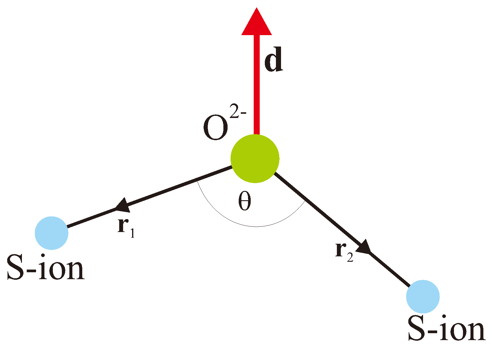
Figure 2.
Dependence of the Fe-Fe, Cr-Cr, Fe-Cr exchange integrals (in K) on the superexchange bond angle in orthoferrites-orthocromites [59].
Figure 2.
Dependence of the Fe-Fe, Cr-Cr, Fe-Cr exchange integrals (in K) on the superexchange bond angle in orthoferrites-orthocromites [59].

Figure 3.
Basic vectors of magnetic structure for sublattice in orthoferrites and orthochromites.
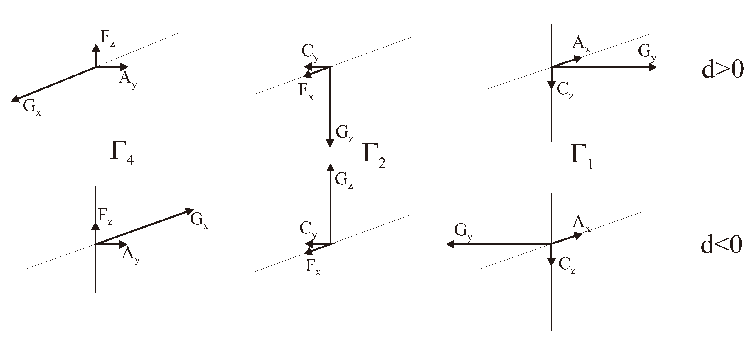
Figure 4.
(a) The MFA phase diagram of weak ferrimagnet YFeCrO given = −4; left and right arrows demonstrate the orientation and magnitude of the magnetization for Fe- and Cr-sublattices, respectively. The outer and inner thin curves mark the compensation points for the net and partial (Fe, Cr) magnetization, respectively. Experimental values of for single crystalline and polycrystalline samples are marked by light and dark circles, respectively. (b) Concentration dependence of the low-temperature magnetization in YFeCrO: experimental data (circles) [23,24], the MFA calculations given = −2 and −4; (c) Concentration dependence of the magnetization and Fe-, Cr- partial contributions in YFeCrO; (d) Temperature dependence of magnetization in YFeCrO: solid curves—experimental data for x = 0.38 (Kadomtseva et al., 1977 [23,24]—curve 1) and for x = 0.4 (Dasari et al., 2012 [79]—curve 2), dotted curve—the MFA calculation for x = 0.4 [79] given = −0.39 K.
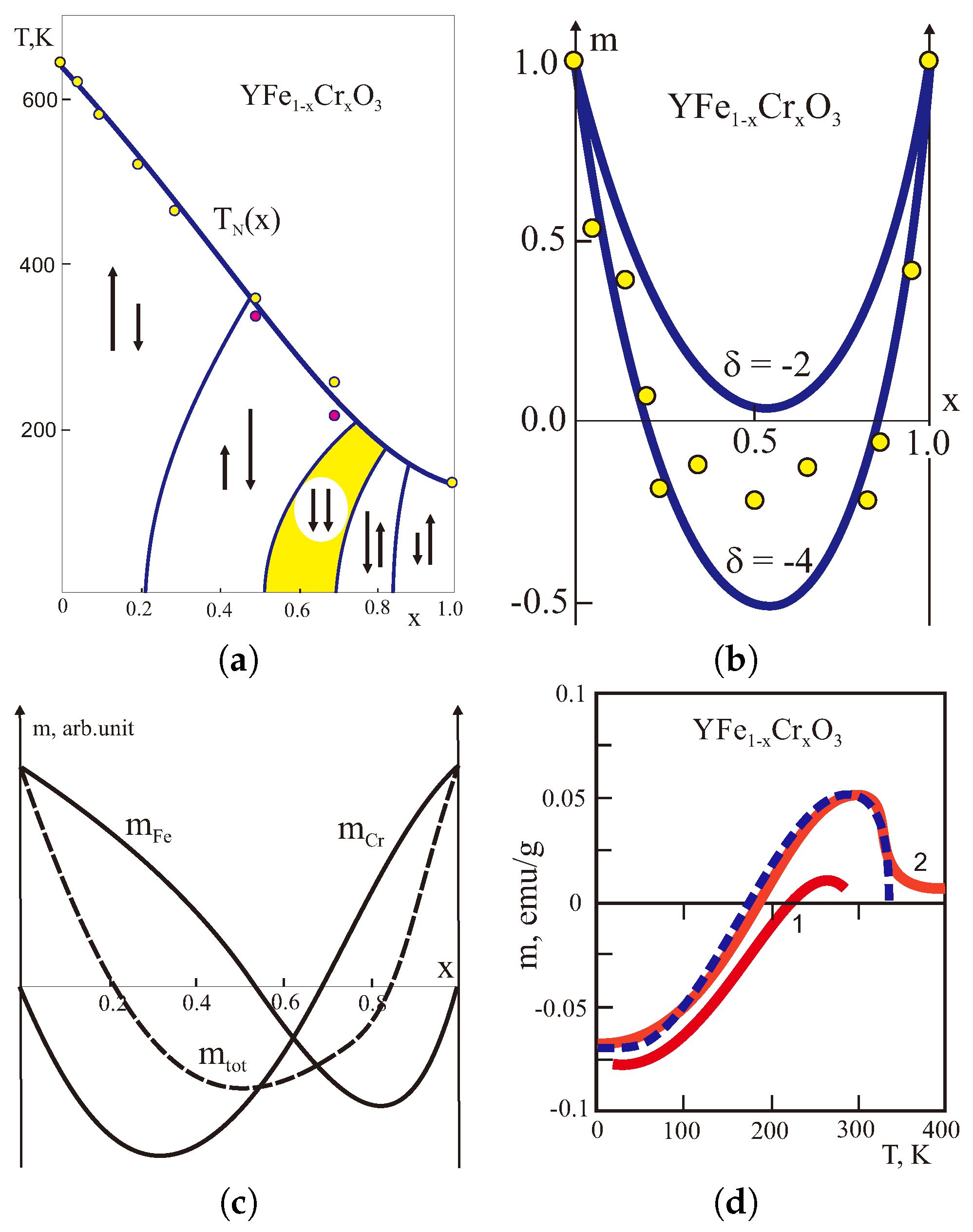
Figure 5.
(a) Concentration dependence of the low-temperature (T = 77 K) magnetization in LuFeCrO: experimental data (circles) [80], the MFA calculations (solid curve) given = −1.5. (b) Temperature dependence of magnetization in LuFeCrO: circles—experimental data [80] given x = 0.6 (1), 0.5 (2), 0.2 (3), 0.1 (4), 0.0 (5), solid curves—the MFA calculations given = −1.5.
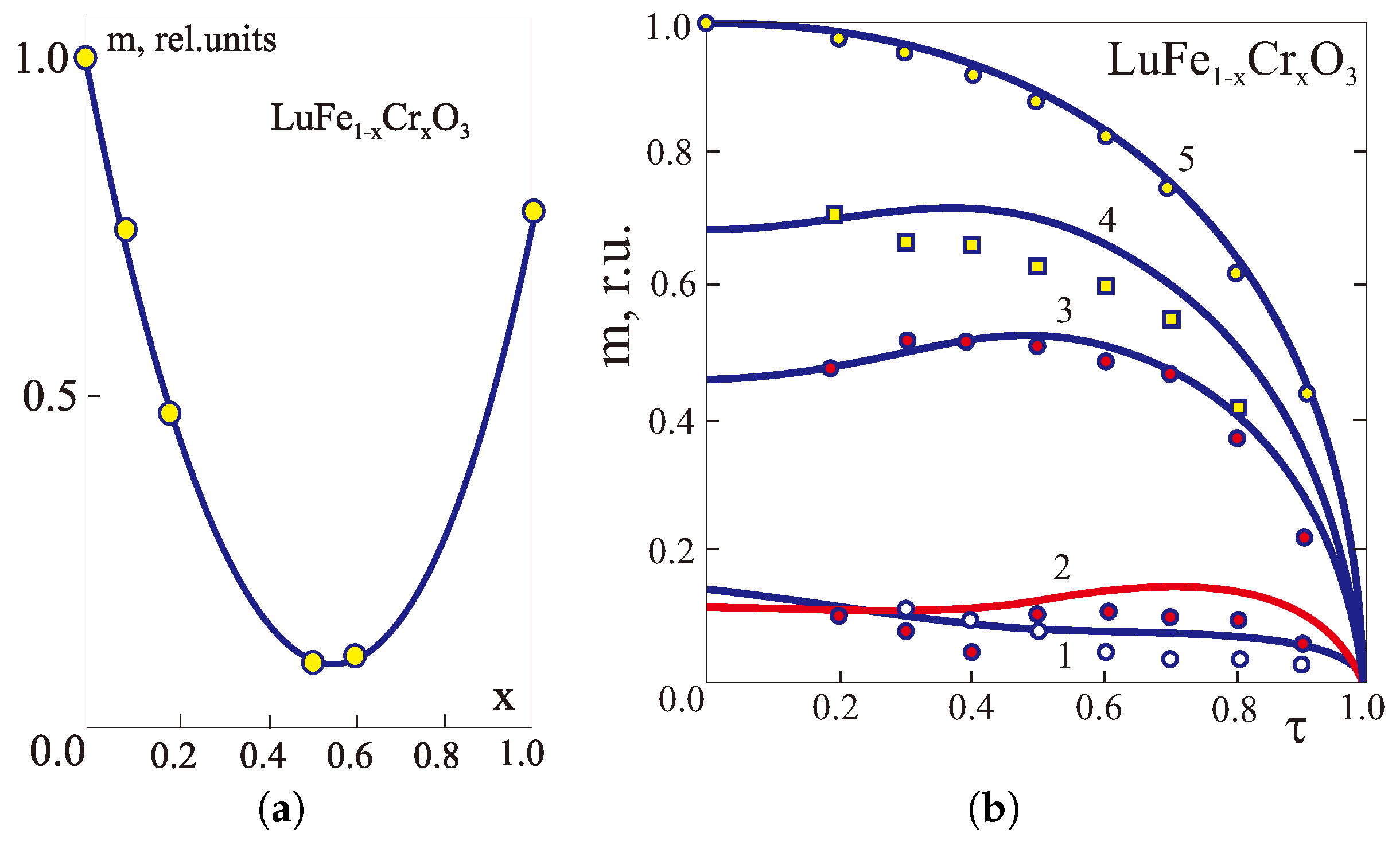
Figure 6.
(a) The MFA simulation of the T-x-phase diagram of the weak ferro(ferri)magnet FeCrBO [78] given = −20.3 K, = 2.0 K, arrows point to orientation of the net weak ferromagnetic moment. Curves 1, 2, 3 mark the compensation points given = = 0.67 K, = −0.67 K (1), −0.75 K (2), −0.90 K (3), respectively. (b) The MFA simulation of the temperature dependence of the net magnetization in FeCrBO [78] given = = − = 0.67 K at different compositions, the insert shows experimental data from ref. [81] taken at external magnetic field 1 T. (c) The MFA simulation of the concentration dependence of the low-temperature magnetization in MnNiCO [77] given and , respectively.

Figure 7.
Two mutual orientations of and vectors in a basal plane of FeF.

Figure 8.
Comparison of simulated (upper panels) and experimental (bottom panel) zero-field NMR spectra in FeF.
Figure 8.
Comparison of simulated (upper panels) and experimental (bottom panel) zero-field NMR spectra in FeF.

Figure 9.
Geometry of the three-center (Cu-O-Cu) two-hole system with ground Cu 3d states.

Figure 10.
The fragment of a typical edge-shared CuO chain with copper and oxygen spin orientation under staggered field applied along x-direction. Note the antiparallel orientation of oxygen Dzyaloshinskii vectors.
Figure 10.
The fragment of a typical edge-shared CuO chain with copper and oxygen spin orientation under staggered field applied along x-direction. Note the antiparallel orientation of oxygen Dzyaloshinskii vectors.


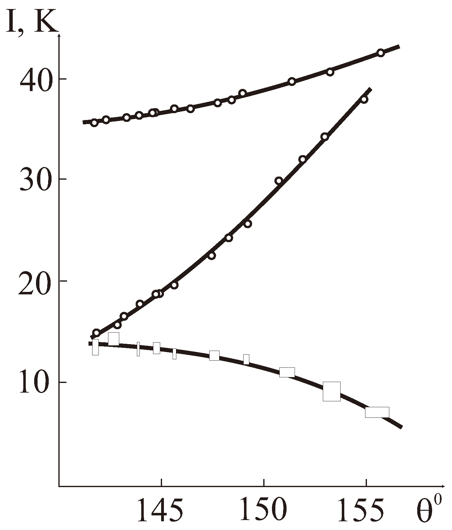
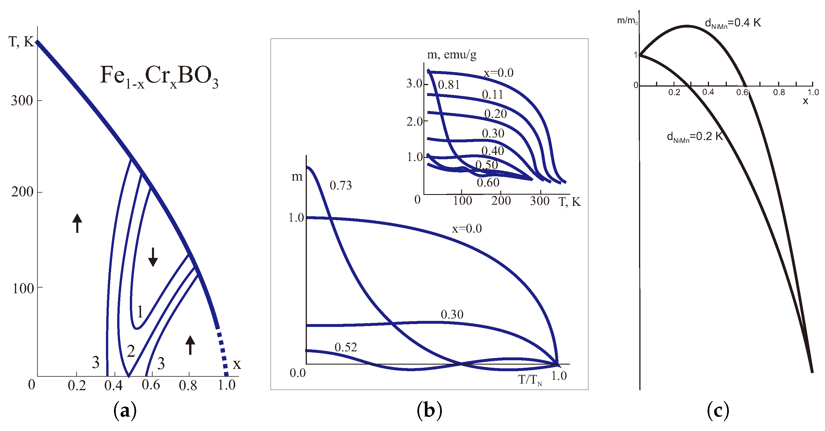
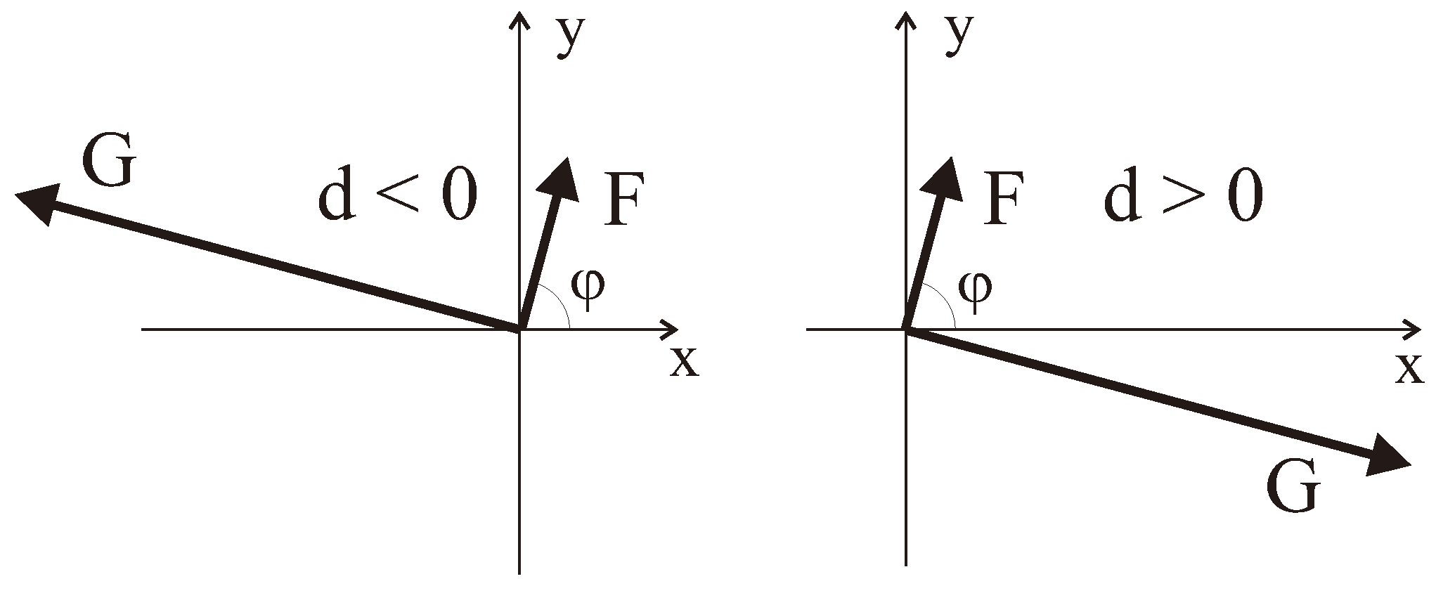
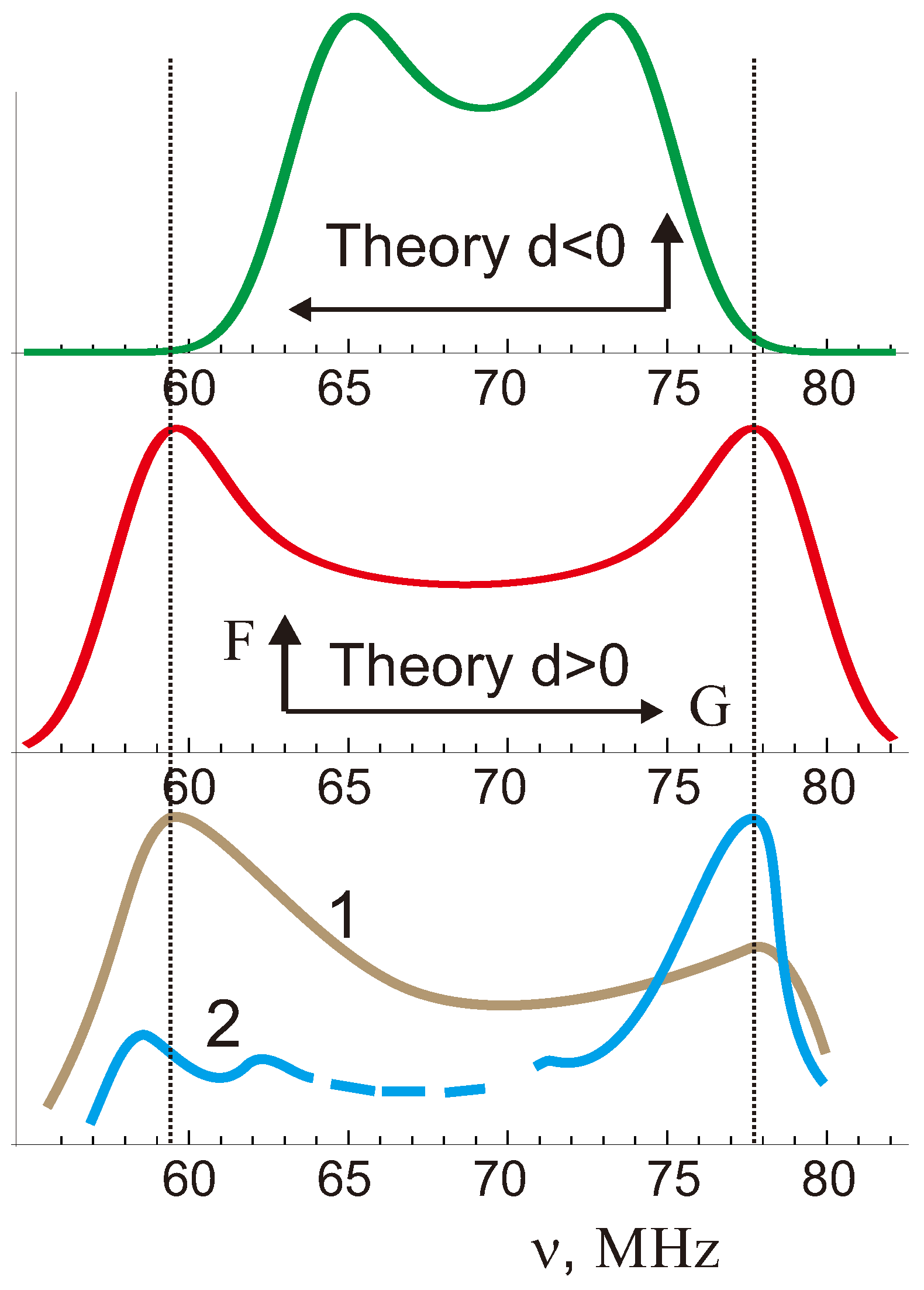
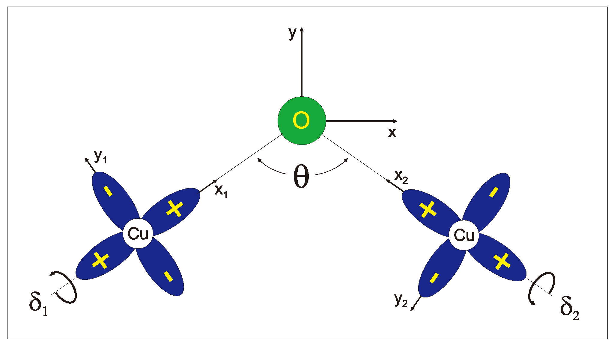
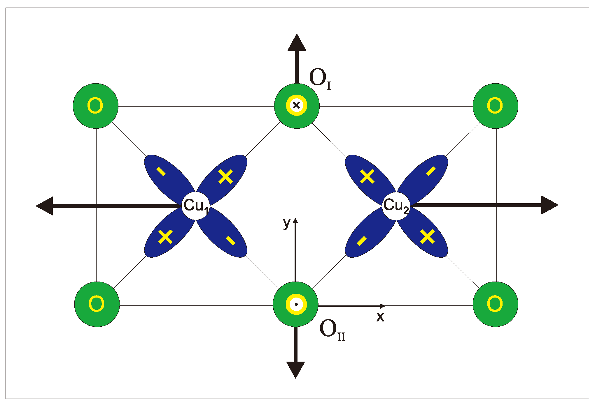
Table 1.
Main exchange and DM coupling parameters in weak ferromagnets (WFMs), I is the exchange integral, is the canting angle. See text for detail.
Table 1.
Main exchange and DM coupling parameters in weak ferromagnets (WFMs), I is the exchange integral, is the canting angle. See text for detail.
| WFM | , Å | , K | I, K (MFA) | , Tesla | , Tesla | d(), K | ||
|---|---|---|---|---|---|---|---|---|
| -FeO [14,15] | 2.111 | 145 | 948 | 54.2 | 870–920 | 1.9–2.2 | 2.3 | |
| YFeO [19] | 2.001 (×2) | 145 | 640 | 36.6 | 640 | 14 | 3.2 | |
| FeBO [20] | 2.028 | 126 | 348 | 19.9 | 300 | 10 | 2.3 | |
| FeF [18] | 1.914 | 153 | 363 | 20.7 | 440 | 4.88 | 1.1 |
Table 2.
Expressions for the X and Y parameters that define the magnitude and the sign of the Dzyaloshinskii vector in pairs of the S-type 3d-ions with local octahedral symmetry. Signs for correspond to the bonding angle .
Table 2.
Expressions for the X and Y parameters that define the magnitude and the sign of the Dzyaloshinskii vector in pairs of the S-type 3d-ions with local octahedral symmetry. Signs for correspond to the bonding angle .
| Ground Sate Configuration | X | Sign X | Y | Sign Y | Excited State Configuration |
|---|---|---|---|---|---|
| (): , , | + | + | |||
| (): , | − | − | − | − | , |
| (): , | − | + |
Table 3.
Sign rules for the Dzyaloshinskii vector in pairs of the S-type 3d-ions with local octahedral symmetry and the bonding angle .
Table 3.
Sign rules for the Dzyaloshinskii vector in pairs of the S-type 3d-ions with local octahedral symmetry and the bonding angle .
| () | () | () | |
|---|---|---|---|
| () | + | − | + |
| () | − | + | + |
| () | + | + | − |
Table 4.
The structural factors for the superexchange coupled Fe–O–Fe pairs in orthoferrites with numerical values for YFeO. See text for detail.
Table 4.
The structural factors for the superexchange coupled Fe–O–Fe pairs in orthoferrites with numerical values for YFeO. See text for detail.
| 1a | = −0.31 | = −0.29 | = 0.41 |
| 1b | = 0.31 | = −0.29 | = 0.41 |
| 3a | = 0.20 | = −0.55 | 0 |
Table 5.
Hidden canting in orthoferrites.
| Orthoferrite | /, Theory [11] | /, exp | /, Theory [11] | /, Exp |
|---|---|---|---|---|
| YFeO | 1.10 | 1.10 ± 0.03 [25] 1.4 ± 0.2 [26,27] 1.1 ± 0.1 [74] | 2.04 | ? |
| HoFeO | 1.16 | 0.85 ± 0.10 [74] | 2.00 | ? |
| TmFeO | 1.10 | 1.25 ± 0.05 [25] | 1.83 | ? |
| YbFeO | 1.11 | 1.22 ± 0.05 [28] | 1.79 | 2.0 ± 0.2 [25] |
Table 6.
Values of the components of the the local field anisotropy tensor for nuclei in positions 1, 2, 3 in FeF (a = 5.333 Å , = 1.486 Å , l = 1.914 Å , x = −0.157 [100]).
Table 6.
Values of the components of the the local field anisotropy tensor for nuclei in positions 1, 2, 3 in FeF (a = 5.333 Å , = 1.486 Å , l = 1.914 Å , x = −0.157 [100]).
| 0 | |||
| 0 | |||
| 0 | 0 | 0 | |
| 0 | |||
© 2019 by the author. Licensee MDPI, Basel, Switzerland. This article is an open access article distributed under the terms and conditions of the Creative Commons Attribution (CC BY) license (http://creativecommons.org/licenses/by/4.0/).
Share and Cite
MDPI and ACS Style
Moskvin, A. Dzyaloshinskii–Moriya Coupling in 3d Insulators. Condens. Matter 2019, 4, 84. https://doi.org/10.3390/condmat4040084
AMA Style
Moskvin A. Dzyaloshinskii–Moriya Coupling in 3d Insulators. Condensed Matter. 2019; 4(4):84. https://doi.org/10.3390/condmat4040084
Chicago/Turabian StyleMoskvin, Alexander. 2019. "Dzyaloshinskii–Moriya Coupling in 3d Insulators" Condensed Matter 4, no. 4: 84. https://doi.org/10.3390/condmat4040084