Electrostatic Interaction of Point Charges in Three-Layer Structures: The Classical Model


Abstract
1. Introduction
2. Formulation of the Problem and Preliminary Remarks
3. General Formulas for in the Dispersionless Approximation
4. Regular Method of Integral Calculation
5. The Particular Case . Series Calculations
- for :
- for :
- for :
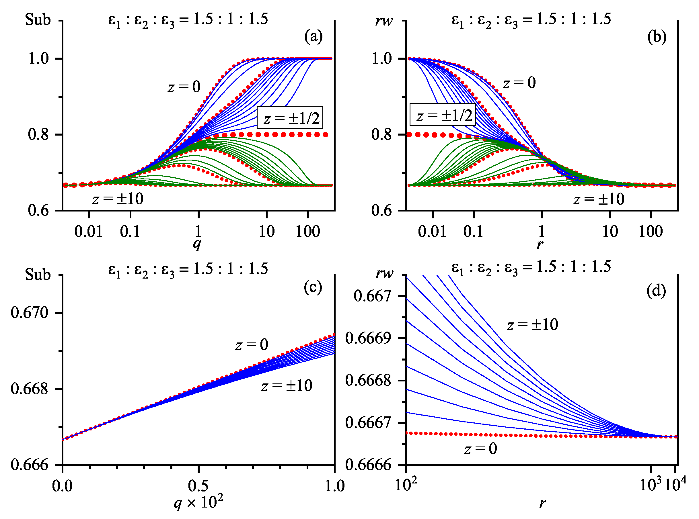
- One can see that the quantity (in essence, the strength of the normalized Coulomb interaction in a three-layer system) strongly depends on z and r. This fact reflects the many-body character of the image forces [111,112] crucially distorting the parent electrostatic interaction in the inhomogeneous (in particular, layered) media.
- For infinitesimally close charges located in the covers’ bulk, i.e., not near the interfaces, the product approaches the appropriate values that characterize the corresponding bulk media i. If the charges are at the interface between media i and j, this value equals , as in much simpler two-layer structures [59]. Thus, when two infinitesimally close charges () cross an interface () between media i and j, the value of the product changes in a step-like manner. To be more precise, it demonstrates two jumps: from to and further to . (Note that such an analysis would be impossible for the “bare” (truly Coulombic) function possessing a conventional pole singularity at .) At , the product —and, hence, the function itself—changes smoothly [as was illustrated in Figure 3a. This transformation was considered in more detail in [59] for a two-layer system. The analysis remains valid for the three-layer system, because two infinitesimally close charges near either of the interfaces “cease to feel” the other interface (as was in the case of the charges in the bulk, where the specific Coulombic singularity “masks” all other interactions in the system), and the three-layer problem transforms into the two-layer one. In the vicinity of interfaces (), we plotted the dependences corresponding to various zs with a small step in order to illustrate how the smoothness of the dependence matches the jumps in the dependence .
- At , all dependences tend to the same limit (see Equation (16)). In terms of dimensional variables, the limit corresponds to both at a fixed L and at a fixed R. Since , the latter interpretation can be regarded as a consequence of two processes: (i) the disappearance of the slab (we leave the ideal conductor case beyond the consideration), so that the three-layer system transforms into a two-layer one; and (ii) the deposition of both charges onto a single interface between two media (1 and 3). From the qualitative viewpoint, this limiting case means that there are no electric force lines in the slab.
- Even for charges located in the depth of any medium, their interaction deviates from the “true” Coulombic dependence () already at rather short distances from each other, i.e., the influence of other media matters.
6. Effective-Exponential Approximation
- The function changes monotonically from at to 1 at , and, as discussed above, it contains no singularities.
- Since Equation (3) involves the Bessel function in the integrand, it is very important for the new function to satisfy the required asymptotics both at and .
7. Long-Range Asymptotic Power Sums
8. Rytova–Keldysh Approximation and Its Modification
8.1. Preliminary Remarks
8.2. RK0 Approximation and Its Modifications
8.3. Original RKA
8.4. Fitting Approximations
8.5. Remarks on the Margin
9. The Case . Coulombic Interaction across the Interlayer
9.1. Preliminary Remarks and Analytical Formulas
9.2. Results of Calculations
10. Conclusions
Author Contributions
Funding
Acknowledgments
Conflicts of Interest
Abbreviations
| CDP | constant-dielectric-permittivity |
| RKA | Rytova–Keldysh approximation |
Appendix A. General Formulas for a Three-Layer System
Appendix Approximation of Dispersionless Dielectric Permittivities
Appendix B. Parameter θ
Appendix C. Constituents of Interaction Energy w(z,z′)
- for :
- for :
- for :
- for :
- for :
- for :
Appendix D. Integrals with the Bessel Function J0(q)

References
- Romanov, Y.A. Theory of characteristic energy losses in thin films. J. Exp. Theor. Phys. 1964, 47, 2119–2133. [Google Scholar]
- Pashitskii, E.A.; Romanov, Y.A. Plasma waves and superconductivity in quantizing semiconducting (semimetallic) films and layered structures. Ukr. Fiz. Zh. 1970, 15, 1594–1606. [Google Scholar]
- Gabovich, A.M.; Pashitskii, E.A.; Uvarova, S.K. Plasmon and exciton superconductivity mechanism in layered structures. Fizika Nizkikh Temperatur 1975, 1, 984–995. [Google Scholar]
- Kornyshev, A.A.; Rubinshtein, A.I.; Vorotyntsev, M.A. Image potential near a dielectric-plasma-like medium interface. Phys. Status Solidi B 1977, 84, 125–132. [Google Scholar] [CrossRef]
- Gabovich, A.M.; Il’chenko, L.G.; Pashitskii, E.A. Electrostatic charge interaction with surfaces of metals and semiconductors. Fiz. Tverd. Tela 1979, 21, 1683–1689. [Google Scholar]
- Gabovich, A.M.; Il’chenko, L.G.; Pashitskii, E.A.; Romanov, Y.A. Electrostatic energy and screened charge interaction near the surface of metals with different Fermi surface shape. Surf. Sci. 1980, 94, 179–203. [Google Scholar] [CrossRef]
- Il’chenko, L.G.; Pashitskii, E.A.; Romanov, Y.A. Electrostatic charge potential in layered systems with spatial dispersion. Fiz. Tverd. Tela 1980, 22, 2700–2710. [Google Scholar]
- Il’chenko, L.G.; Pashitskii, E.A.; Romanov, Y.A. Charge interaction in layered systems. Fiz. Tverd. Tela 1980, 22, 3395–3401. [Google Scholar]
- Gabovich, A.M.; Il’chenko, L.G.; Pashitskii, E.A. Energy spectrum of electrons above a thin liquid helium film in a clamping electrical field. J. Exp. Theor. Phys. 1981, 81, 2063–2069. [Google Scholar]
- Kornyshev, A.A.; Vorotyntsev, M.A.; Ulstrup, J. The effect of spatial dispersion of the dielectric permittivity on the capacitance of thin insulating films: non-linear dependence of the inverse capacitance on film thickness. Thin Solid Films 1981, 75, 105–118. [Google Scholar] [CrossRef]
- Il’chenko, L.G.; Pashitskii, E.A.; Romanov, Y.A. Charge interaction in layered systems with spatial dispersion. Surf. Sci. 1982, 121, 375–395. [Google Scholar] [CrossRef]
- Gabovich, A.M.; Il’chenko, L.G.; Pashitskii, E.A. Image force and electron spectrum at the surface of liquid helium. Surf. Sci. 1983, 130, 373–394. [Google Scholar] [CrossRef]
- Gabovich, A.M.; Rozenbaum, V.M. Image forces and quantum states in semiconductor heterostructures. Fiz. Tekhn. Polup. 1984, 18, 498–501. [Google Scholar]
- Bechstedt, F.; Enderlein, R. Dielectric screening, polar phonons, and longitudinal electronic excitations of quantum well double heterostructures. Application to light scattering from charge density fluctuations. Phys. Status Solidi B 1985, 131, 53–66. [Google Scholar] [CrossRef]
- Gabovich, A.M.; Rozenbaum, V.M.; Voitenko, A.I. Dynamical image forces in three-layer systems and field emission. Surf. Sci. 1987, 186, 523–549. [Google Scholar] [CrossRef]
- Pokatilov, E.P.; Fomin, V.M.; Beril, S.I. Oscillatory Excitations, Polarons and Excitons in Multilayer Systems and Superlattices; Shtiintsa: Kishinev, Moldova, 1990. [Google Scholar]
- Pokatilov, E.P.; Beril, S.I.; Semenovskaya, N.N.; Fahood, M. Charge carrier energy spectrum in multi-layer structures and superlattices in the field of the self-action potential. Phys. Status Solidi B 1990, 158, 165–174. [Google Scholar] [CrossRef]
- Wendler, L.; Hartwig, B. The effect of the image potential on the binding energy of hydrogenic impurities in semiconductor quantum wells. J. Phys. Condens. Matter 1990, 2, 8847–8852. [Google Scholar] [CrossRef]
- Wendler, L.; Bechstedt, F.; Fiedler, M. Quasi-two-dimensional screening of the electron-hole interaction in modulation-doped quantum wells. Phys. Status Solidi B 1990, 159, 143–154. [Google Scholar] [CrossRef]
- Bah, M.L.; Akjouj, A.; Dobrzynski, L. Response functions in layered dielectric media. Surf. Sci. Rep. 1992, 16, 95–131. [Google Scholar] [CrossRef]
- Voitenko, A.I.; Gabovich, A.M.; Rozenbaum, V.M. Dynamic image forces and tunneling in three-layer systems. Fiz. Nizk. Temp. 1996, 22, 86–98. [Google Scholar]
- Basko, D.; La Rocca, G.C.; Bassani, F.; Agranovich, V.M. Förster energy transfer from a semiconductor quantum well to an organic material overlayer. Eur. Phys. J. B 1999, 8, 353–362. [Google Scholar] [CrossRef]
- Gabovich, A.M.; Reznikov, Y.A.; Voitenko, A.I. Excess nonspecific Coulomb ion adsorption at the metal electrode/electrolyte solution interface: Role of the surface layer. Phys. Rev. E 2006, 73, 021606. [Google Scholar] [CrossRef] [PubMed]
- Kovalev, V.M.; Chaplik, A.V. Screening effects and Friedel oscillations in quantum-well nanostructures. J. Exp. Theor. Phys. 2008, 134, 980–987. [Google Scholar] [CrossRef]
- Slater, J.C. The electronic structure of metals. Rev. Mod. Phys. 1934, 6, 209–280. [Google Scholar] [CrossRef]
- Herring, C.; Nichols, M.H. Thermionic emission. Rev. Mod. Phys. 1949, 21, 185–270. [Google Scholar] [CrossRef]
- Jennings, P.J.; Jones, R.O. Beyond the method of images – the interaction of charged particles with real surfaces. Adv. Phys. 1988, 37, 341–358. [Google Scholar] [CrossRef]
- Kiejna, A.; Wojciechowski, K.F. Metal Surface Electron Physics; Pergamon Press: Oxford, UK, 1996. [Google Scholar]
- Andrei, E.Y. (Ed.) Two-Dimensional Electron systems on Helium and Other Cryogenic Substrates; Kluwer Academic: Dordrecht, The Netherlands, 1997. [Google Scholar]
- Monarkha, Y.; Kono, K. Two-Dimensional Coulomb Liquids and Solids; Springer: New York, NY, USA, 2004. [Google Scholar]
- Gabovich, A.M. Image forces in physics and chemistry of surfaces: certain fundamental aspects. Chem. Phys. Technol. Surf. 2010, 1, 72–86. [Google Scholar]
- Gabovich, A.M.; Li, M.S.; Szymczak, H.; Voitenko, A.I. Image forces for a point-like dipole near a plane metal surface: An account of the spatial dispersion of dielectric permittivity. Surf. Sci. 2012, 606, 510–515. [Google Scholar] [CrossRef]
- Barker, J.R.; Martinez, A. Image charge models for accurate construction of the electrostatic self-energy of 3D layered nanostructure devices. J. Phys. Condens. Matter 2018, 30, 134002. [Google Scholar] [CrossRef]
- Wojciechowski, K.F. The quantum theory of adsorption on metal surfaces. Progr. Surf. Sci. 1971, 1, 65–104. [Google Scholar] [CrossRef]
- Meissner, G.; Namaizawa, H.; Voss, M. Stability and image-potential-induced screening of electrons in a three-layer structure. Phys. Rev. B 1976, 13, 1370–1376. [Google Scholar] [CrossRef]
- Lau, K.H.; Kohn, W. Indirect long-range oscillatory interaction between adsorbed atoms. Surf. Sci. 1978, 75, 69–85. [Google Scholar] [CrossRef]
- Le Bosse, J.C.; Lopez, J.; Rousseau-Violet, J. Interaction energy between two identical atoms cnemisorbed on a normal metal. Surf. Sci. 1978, 72, 125–139. [Google Scholar] [CrossRef]
- Vorotyntsev, M.A.; Kornyshev, A.A. Electrostatic interaction at the metal/insulator interface. J. Exp. Theor. Phys. 1980, 78, 1008–1019. [Google Scholar]
- Kornyshev, A.A. Non-local enhancement of the dipole-dipole interaction at the interface of two dielectrics. J. Electroanal. Chem. 1988, 255, 297–302. [Google Scholar] [CrossRef]
- Vorotyntsev, M.A.; Ivanov, S.N. Image force energy and ion interaction with the charge group near a contact insulator/electrolyte solution. Elektrokhim 1989, 25, 550–554. [Google Scholar]
- Merrick, M.L.; Luo, W.; Fichthorn, K.A. Substrate-mediated interactions on solid surfaces: theory, experiment, and consequences for thin-film morphology. Prog. Surf. Sci. 2003, 72, 117–134. [Google Scholar] [CrossRef]
- Kokalj, A. Electrostatic model for treating long-range lateral interactions between polar molecules adsorbed on metal surfaces. Phys. Rev. B 2011, 84, 045418. [Google Scholar] [CrossRef]
- Gabovich, A.M.; Voitenko, A.I. Electrostatic charge-charge and dipole-dipole interactions near the surface of a medium with screening non-locality (Review Article). Fiz. Nizk. Temp. 2016, 42, 841–853. [Google Scholar] [CrossRef][Green Version]
- Chaplik, A.V. Possible crystallization of charge carriers in low-density inversion layers. J. Exp. Theor. Phys. 1972, 62, 746–753. [Google Scholar]
- Shikin, V.B.; Monarkha, Y.P. On the interaction of surface electrons in liquid helium with oscillations of the vapor-liquid interface. J. Low Temp. Phys. 1974, 16, 193–208. [Google Scholar] [CrossRef]
- Shevchenko, S.I. Theory of superconductivity for systems with pairing of spatially-separated electrons and holes. Fiz. Nizk. Temp. 1976, 2, 505–516. [Google Scholar]
- Lozovik, Y.E.; Yudson, V.I. A new mechanism for superconductivity: pairing between spatially separated electrons and holes. J. Exp. Theor. Phys. 1976, 71, 738–753. [Google Scholar]
- Keldysh, L.V. Coulomb interaction in thin semiconductor and semimetal films. Pis’ma J. Exp. Theor. Phys. 1979, 29, 716–719. [Google Scholar]
- Monarkha, Y.P.; Shikin, V.B. Low-dimensional electron systems at liquid helium surface (Review article). Fiz. Nizk. Temp. 1982, 8, 563–600. [Google Scholar]
- Shikin, V.B.; Monarkha, Y.P. Two-Dimensional Charged Systems in Helium; Nauka: Moscow, Russia, 1989. [Google Scholar]
- Agranovich, V.M.; Basko, D.M.; La Rocca, G.C.; Bassani, F. Excitons and optical nonlinearities in hybrid organic-inorganic nanostructures. J. Phys. Condens. Matter 1998, 10, 9369–9400. [Google Scholar] [CrossRef]
- Ando, T.; Fowler, A.B.; Stern, F. Electronic properties of two-dimensional systems. Rev. Mod. Phys. 1982, 54, 437–672. [Google Scholar] [CrossRef]
- Braun, O.M.; Medvedev, V.K. Interaction between particles adsorbed on the metal surface. Usp. Fiz. Nauk 1989, 157, 631–656. [Google Scholar] [CrossRef]
- Persson, B.N.J. Ordered structures and phase transitions in adsorbed layers. Surf. Sci. Rep. 1992, 15, 1–135. [Google Scholar] [CrossRef]
- Kaganer, V.M.; Möhwald, H.; Dutta, P. Structure and phase transitions in Langmuir monolayers. Rev. Mod. Phys. 1999, 71, 779–819. [Google Scholar] [CrossRef]
- French, R.H.; Parsegian, V.A.; Podgornik, R.; Rajter, R.F.; Jagota, A.; Luo, J.; Asthagiri, D.; Chaudhury, M.K.; Chiang, Y.-M.; Granick, S.; et al. Long range interactions in nanoscale science. Rev. Mod. Phys. 2010, 82, 1887–1944. [Google Scholar] [CrossRef]
- Antczak, G.; Ehrlich, G. Surface Diffusion. Metals, Metal Atoms, and Clusters; Cambridge University Press: Cambridge, UK, 2010. [Google Scholar]
- Krim, J. Friction and energy dissipation mechanisms in adsorbed molecules and molecularly thin films. Adv. Phys. 2012, 61, 155–323. [Google Scholar] [CrossRef]
- Gabovich, A.M.; Voitenko, A.I. The ’non-Coulombic’ character of classical electrostatic interaction between charges near interfaces. Eur. J. Phys. 2018, 39, 045203. [Google Scholar] [CrossRef]
- Colinge, J.P.; Colinge, C.A. Physics of Semiconductor Devices; Kluwer Academic: New York, NY, USA, 2002. [Google Scholar]
- Fu, Y. Physical Models of Semiconductor Quantum Devices; Springer: Dordrecht, The Netherlands, 2014. [Google Scholar]
- Vasko, F.T.; Kuznetsov, A.V. Electronic States and Optical Transitions in Semiconductor Heterostructures; Springer: New York, NY, USA, 1999. [Google Scholar]
- Manasreh, O. Semiconductor Heterojunctions and Nanostructures; McGraw-Hill: New York, NY, USA, 2005. [Google Scholar]
- Burg, G.W.; Prasad, N.; Kim, K.; Taniguchi, T.; Watanabe, K.; MacDonald, A.H.; Register, L.F.; Tutuc, E. Strongly enhanced tunneling at total charge neutrality in double-bilayer graphene-WSe2 heterostructures. Phys. Rev. Lett. 2018, 120, 177702. [Google Scholar] [CrossRef] [PubMed]
- Song, J.C.W.; Gabor, N.M. Electron quantum metamaterials in van der Waals heterostructures. Nat. Nanotechnol. 2018, 13, 986–993. [Google Scholar] [CrossRef] [PubMed]
- Rivera, P.; Yu, H.; Seyler, K.L.; Wilson, N.P.; Yao, W.; Xu, X. Interlayer valley excitons in heterobilayers of transition metal dichalcogenides. Nat. Nanotechnol. 2018, 13, 1004–1015. [Google Scholar] [CrossRef] [PubMed]
- Katriel, J. Spectrum of two-dimensional excitons in heterojunction superlattices. Phys. Lett. A 1984, 101, 158–160. [Google Scholar] [CrossRef]
- Fomin, V.M.; Pokatilov, E.P. Excitons in multi-layer systems. Phys. Status Solidi B 1985, 129, 203–209. [Google Scholar] [CrossRef]
- Pokatilov, E.P.; Beril, S.I.; Fomin, V.M.; Pogorilko, G.A. Wannier-Mott exciton states in two-layer periodic structures. Phys. Status Solidi B 1985, 130, 619–628. [Google Scholar] [CrossRef]
- Keldysh, L.V. Excitons and polaritons in semiconductor/insulator quantun wells and superlattices. Superlattices Microstruct. 1988, 4, 637–642. [Google Scholar] [CrossRef]
- Tran Thoai, D.B. Exciton binding energy in semiconductor quantum wells and in heterostructures. Physica B 1990, 164, 295–299. [Google Scholar] [CrossRef]
- Pokatilov, E.P.; Beril, S.I.; Fomin, V.M.; Kalinovskii, V.V. The size-quantized states of the Wannier-Mott exciton in structures with superthin films of CdTe. Phys. Status Solidi B 1990, 161, 603–612. [Google Scholar] [CrossRef]
- Berkelbach, T.C.; Reichman, D.R. Optical and excitonic properties of atomically thin transition-metal dichalcogenides. Annu. Rev. Condens. Matter Phys. 2018, 9, 379–396. [Google Scholar] [CrossRef]
- Brunetti, M.N.; Berman, O.L.; Kezerashvili, R.Y. Optical properties of excitons in buckled two-dimensional materials in an external electric field. Phys. Rev. B 2018, 98, 125406. [Google Scholar] [CrossRef]
- Wang, G.; Chernikov, A.; Glazov, M.M.; Heinz, T.F.; Marie, X.; Amand, T.; Urbaszek, B. Colloquium: Excitons in atomically thin transition metal dichalcogenides. Rev. Mod. Phys. 2018, 90, 021001. [Google Scholar] [CrossRef]
- Zhang, J.-Z.; Ma, J.-Z. Two-dimensional excitons in monolayer transition metal dichalcogenides from radial equation and variational calculations. J. Phys. Condens. Matter 2019, 31, 105702. [Google Scholar] [CrossRef]
- Scharf, B.; Tuan, D.V.; Žutić, I.; Dery, H. Dynamical screening in monolayer transition-metal dichalcogenides and its manifestations in the exciton spectrum. J. Phys. Condens. Matter 2019, 31, 203001. [Google Scholar] [CrossRef]
- Ávalos Ovando, O.; Mastrogiuseppe, D.; Ulloa, S.E. Lateral heterostructures and one-dimensional interfaces in 2D transition metal dichalcogenides. J. Phys. Condens. Matter 2019, 31, 213001. [Google Scholar] [CrossRef]
- Lozovik, Y.E.; Yudson, V.I. Feasibility of superfluidity of paired spatially-separated paired electrons and holes; a new superconductivity mechanism. Pis’ma J. Exp. Theor. Phys. 1975, 22, 556–559. [Google Scholar]
- Kulik, I.O.; Shevchenko, S.I. Excitonic pairing and superconductivity in layered systems. Fiz. Nizk. Temp. 1976, 2, 1405–1426. [Google Scholar]
- Shevchenko, S.I.; Kulik, I.O. Electrodynamics of exciton pairing in low-dimensionality crystals without inversion centers. Pis’ma J. Exp. Theor. Phys. 1976, 23, 171–173. [Google Scholar]
- Shevchenko, S.I. Ginzburg-Landau equations and quantum coherent phenomena in systems with electron-hole pairing. Fiz. Nizk. Temp. 1977, 3, 605–623. [Google Scholar]
- Shevchenko, S.I. Phase diagram of systems with pairing of spatially separated electrons and holes. Phys. Rev. Lett. 1994, 72, 3242–3245. [Google Scholar] [CrossRef] [PubMed]
- Fil, D.V.; Shevchenko, S.I. Electron-hole superconductivity (Review Article). Fiz. Nizk. Temp. 2018, 44, 1111–1160. [Google Scholar] [CrossRef]
- Berman, O.L.; Kezerashvili, R.Y. Superfluidity of dipolar excitons in a transition metal dichalcogenide double layer. Phys. Rev. B 2017, 96, 094502. [Google Scholar] [CrossRef]
- Saberi-Pouya, S.; Zarenia, M.; Perali, A.; Vazifehshenas, T.; Peeters, F.M. High-temperature electron-hole superfluidity with strong anisotropic gaps in double phosphorene monolayers. Phys. Rev. B 2018, 97, 174503. [Google Scholar] [CrossRef]
- Leiderer, P.; Ebner, W.; Shikin, V.B. Macroscopic electron dimples on the surface of liquid helium. Surf. Sci. 1982, 113, 405–411. [Google Scholar] [CrossRef]
- Kovdrya, Y.Z. One- and zero-dimensional electron systems over liquid helium (Review Article). Fiz. Nizk. Temp. 2003, 29, 107–144. [Google Scholar] [CrossRef]
- Leiderer, P.; Wanner, M.; Schoepe, W. Ions at the critical interface of 3He-4He mixtures. J. Phys. (Paris) Colloq. 1978, 39, 1328–1333. [Google Scholar] [CrossRef][Green Version]
- Barenghi, C.F.; Mellor, C.J.; Muirhead, C.M.; Vinen, W.F. Experiments on ions trapped below the surface of superfluid 4He. J. Phys. C 1986, 19, 1135–1144. [Google Scholar] [CrossRef]
- Zangi, R. Water confined to a slab geometry: A review of recent computer simulation studies. J. Phys. Condens. Matter 2004, 16, S5371–S5388. [Google Scholar] [CrossRef]
- Manciu, M.; Ruckenstein, E. On the interactions of ions with the air/water interface. Langmuir 2005, 21, 11312–11319. [Google Scholar] [CrossRef] [PubMed]
- Kornyshev, A.A.; Lee, D.J.; Leikin, S.; Wynveen, A. Structure and interactions of biological helices. Rev. Mod. Phys. 2007, 79, 943–996. [Google Scholar] [CrossRef]
- Choy, J.-H.; Kwon, S.-J.; Park, G.-S. High-Tc superconductors in the two-dimensional limit: [(Py-CnH2n+1)2HgI4]-Bi2Sr2Cam-1CumOy (m = 1 and 2). Science 1998, 280, 1589–1592. [Google Scholar] [CrossRef]
- Kerman, K.; Ramanathan, S. Performance of solid oxide fuel cells approaching the two-dimensional limit. J. Appl. Phys. 2014, 115, 174307. [Google Scholar] [CrossRef]
- Duong, D.L.; Yun, S.J.; Lee, Y.H. van der Waals layered materials: opportunities and challenges. ACS Nano 2017, 11, 11803–11830. [Google Scholar] [CrossRef] [PubMed]
- Durnev, M.V.; Glazov, M.M. Excitons and trions in two-dimensional semiconductors based on transition metal dichalcogenides. Usp. Fiz. Nauk 2018, 188, 913–934. [Google Scholar] [CrossRef]
- Florian, M.; Hartmann, M.; Steinhoff, A.; Klein, J.; Holleitner, A.W.; Finley, J.J.; Wehling, T.O.; Kaniber, M.; Gies, C. The dielectric impact of layer distances on exciton and trion binding energies in van der Waals heterostructures. Nano Lett. 2018, 18, 2725–2732. [Google Scholar] [CrossRef] [PubMed]
- Kotov, V.N.; Uchoa, B.; Pereira, V.M.; Guinea, F.; Castro Neto, A.H. Electron-electron interactions in graphene: current status and perspectives. Rev. Mod. Phys. 2012, 84, 1067–1125. [Google Scholar] [CrossRef]
- Basov, D.N.; Fogler, M.M.; Lanzara, A.; Wang, F.; Zhang, Y. Colloquium: Graphene spectroscopy. Rev. Mod. Phys. 2014, 86, 959–994. [Google Scholar] [CrossRef]
- Cudazzo, P.; Tokatly, I.V.; Rubio, A. Dielectric screening in two-dimensional insulators: Implications for excitonic and impurity states in graphane. Phys. Rev. B 2011, 84, 085406. [Google Scholar] [CrossRef]
- Andrews, L.C.; Shivamoggi, B.K. Integral Transforms in Science for Engineers; Macmillan: New York, NY, USA, 1988. [Google Scholar]
- Debnath, L.; Bhatta, D. Integral Transforms and Their Applications, 2nd ed.; Chapman and Hall/CRC: Boca Raton, FL, USA, 2007. [Google Scholar]
- Canel, E.; Matthews, M.P.; Zia, R.K.P. Screening in very thin films. Phys. Kondens. Mater. 1972, 15, 191–200. [Google Scholar] [CrossRef]
- Ferry, D.; Goodnick, S.; Bird, J. Transport in Nanostructures, 2nd ed.; Cambridge University Press: Cambridge, UK, 2009. [Google Scholar]
- Smythe, W.R. Static and Dynamic Electricity; McGraw-Hill: New York, NY, USA, 1950. [Google Scholar]
- Kittel, C. Introduction to Solid State Physics; John Wiley and Sons: New York, NY, USA, 2005. [Google Scholar]
- Lüpke, G. Characterization of semiconductor interfaces by second-harmonic generation. Surf. Sci. Rep. 1999, 35, 75–161. [Google Scholar] [CrossRef]
- Ogale, S.B. Thin Fiims and Heterostructures for Oxide Electronics; Springer: New York, NY, USA, 2010. [Google Scholar]
- Lamberti, C.; Agostini, G. (Eds.) Characterization of Semiconductor Heterostructures and Nanostructures, 2nd ed.; Elsevier: Oxford, UK, 2013. [Google Scholar]
- Gadzuk, J.W. The effects of screened exchange and correlation on the surface potential of an electron gas. Surf. Sci. 1968, 11, 465–478. [Google Scholar] [CrossRef]
- Inkson, J.C. The electron-electron interaction near an interface. Surf. Sci. 1971, 28, 69–76. [Google Scholar] [CrossRef]
- Rytova, N.S. Screened potential of a charge in a thin film. Vestn. Mosk. Univ. 1967, 3, 30–37. [Google Scholar]
- Berkelbach, T.C.; Hybertsen, M.S.; Reichman, D.R. Theory of neutral and charged excitons in monolayer transition metal dichalcogenides. Phys. Rev. B 2013, 88, 045318. [Google Scholar] [CrossRef]
- Rodin, A.S.; Carvalho, A.; Castro Neto, A.H. Excitons in anisotropic two-dimensional semiconducting crystals. Phys. Rev. B 2014, 90, 075429. [Google Scholar] [CrossRef]
- Kylänpää, I.; Komsa, H.-P. Binding energies of exciton complexes in transition metal dichalcogenide monolayers and effect of dielectric environment. Phys. Rev. B 2015, 92, 205418. [Google Scholar] [CrossRef]
- Deng, T.; Su, H. Orbital-dependent electron-hole interaction in graphene and associated multi-layer structures. Sci. Rep. 2015, 5, 17337. [Google Scholar] [CrossRef]
- Thygesen, K.S. Calculating excitons, plasmons, and quasiparticles in 2D materials and van der Waals heterostructures. 2D Mater 2017, 4, 022004. [Google Scholar] [CrossRef]
- Han, B.; Robert, C.; Courtade, E.; Manca, M.; Shree, S.; Amand, T.; Renucci, P.; Taniguchi, T.; Watanabe, K.; Marie, X.; et al. Exciton states in monolayer MoSe2 and MoTe2 probed by upconversion spectroscopy. Phys. Rev. X 2018, 8, 031073. [Google Scholar] [CrossRef]
- Abramowitz, M.; Stegun, I.A. (Eds.) Handbook of Mathematical Functions with Formulas, Graphs and Mathematical Tables; US Government Printing Office: Wasington, DC, USA, 1964.
- Luke, Y.I. Mathematical Functions and Their Approximations; Academic Press: New York, NY, USA, 1975. [Google Scholar]
- Bastard, G. Hydrogenic impurity states in a quantum well: A simple model. Phys. Rev. B 1981, 24, 47l4–4722. [Google Scholar] [CrossRef]
- Barcellona, P.; Bennett, R.; Buhmann, S.Y. Manipulating the Coulomb interaction: A Green’s function perspective. J. Phys. Commun. 2018, 2, 035027. [Google Scholar] [CrossRef]
- Gomes, L.C.; Trevisanutt, P.E.; Carvalho, A.; Rodin, A.S.; Castro Neto, A.H. Strongly bound Mott-Wannier excitons in GeS and GeSe monolayers. Phys. Rev. B 2016, 94, 155428. [Google Scholar] [CrossRef]
- Cavalcante, L.S.R.; Chaves, A.; Van Duppen, B.; Peeters, F.M.; Reichman, D.R. Electrostatics of electron-hole interactions in van der Waals heterostructures. Phys. Rev. B 2018, 97, 125427. [Google Scholar] [CrossRef]
- Cho, Y.; Berkelbach, T.C. Environmentally sensitive theory of electronic and optical transitions in atomically thin semiconductors. Phys. Rev. B 2018, 97, 041409. [Google Scholar] [CrossRef]
- Stern, F.; Howard, W.E. Properties of semiconductor surface inversion layers in the electric quantum limit. Phys. Rev. 1967, 163, 816–835. [Google Scholar] [CrossRef]
- Fetter, A.L. Electrodynamics of a layered electron gas. I. Single layer. Ann. Phys. 1973, 81, 367–393. [Google Scholar] [CrossRef]
- Keldysh, L.V. Excitons in semiconductor-dielectric nanostructures. Phys. Status Solidi A 1997, 164, 3–11. [Google Scholar] [CrossRef]
- Chernikov, A.; Berkelbach, T.C.; Hill, H.M.; Rigosi, A.; Li, Y.; Aslan, O.B.; Reichman, D.R.; Hybertsen, M.S.; Heinz, T.F. Exciton binding energy and nonhydrogenic Rydberg series in monolayer WS2. Phys. Rev. Lett. 2014, 113, 076802. [Google Scholar] [CrossRef]
- Ritchie, R.H.; Marusak, A.L. The surface plasmon dispersion relation for an electron gas. Surf. Sci. 1966, 4, 234–240. [Google Scholar] [CrossRef]
- Gadzuk, J.W. A comparison between the Fermi-Thomas and quantum dielectric response of a metal surface to a static point charge. Surf. Sci. 1970, 23, 58–68. [Google Scholar] [CrossRef]
- Beck, D.E.; Celli, V. Linear response of a metal to an external charge distribution. Phys. Rev. B 1970, 2, 2955–2960. [Google Scholar] [CrossRef]
- Heinrichs, J. Response of metal surfaces to static and moving point charges and to polarizable charge distributions. Phys. Rev. B 1973, 8, 1346–1364. [Google Scholar] [CrossRef]
- Echenique, P.M.; Pendry, J.B. Theory of image states at metal surfaces. Progr. Surf. Sci. 1989, 32, 111–172. [Google Scholar] [CrossRef]
- Kirzhnits, D.A. General properties of electromagnetic response functions. Usp. Fiz. Nauk 1987, 152, 399–422. [Google Scholar] [CrossRef]
- Erdélyi, A.; Magnus, W.; Oberhettinger, F.; Tricomi, F. Tables of Integral Transforms, Vol. 2; McGraw Hill: New York, NY, USA, 1954. [Google Scholar]
- Gradshteyn, I.S.; Ryzhik, I.M. (Eds.) Table of Intergrals, Series and Products; Academic Press: San Diego, CA, USA, 2000. [Google Scholar]
- Sidyakin, A.V. Calculation of the polarization contribution to the energy of interaction of a charge with the surface of a metal. J. Exp. Theor. Phys. 1970, 58, 573–581. [Google Scholar]
- Gabovich, A.M.; Il’chenko, L.G.; Pashitskii, E.A.; Romanov, Y.A. Charge screening and electron density Friedel oscillations in metals with different Fermi surface shape. J. Exp. Theor. Phys. 1978, 75, 249–264. [Google Scholar]


| Structure | Specific Feature | ||||
|---|---|---|---|---|---|
| A | 1 | 2 | 5 | ||
| B | 2 | 1 | 5 | ||
| C | 1 | 5 | 2 | ||
| D | 1 | 1.5 | 1 | ||
| E | 1.5 | 1 | 1.5 | ||
| F | 1 | 10 | 1 | ||
| G | 10 | 1 | 10 | ||
| H | 1 | 100 | 1 | ||
| I | 100 | 1 | 100 |
© 2019 by the authors. Licensee MDPI, Basel, Switzerland. This article is an open access article distributed under the terms and conditions of the Creative Commons Attribution (CC BY) license (http://creativecommons.org/licenses/by/4.0/).
Share and Cite
Gabovich, A.M.; Voitenko, A.I. Electrostatic Interaction of Point Charges in Three-Layer Structures: The Classical Model. Condens. Matter 2019, 4, 44. https://doi.org/10.3390/condmat4020044
Gabovich AM, Voitenko AI. Electrostatic Interaction of Point Charges in Three-Layer Structures: The Classical Model. Condensed Matter. 2019; 4(2):44. https://doi.org/10.3390/condmat4020044
Chicago/Turabian StyleGabovich, Alexander M., and Alexander I. Voitenko. 2019. "Electrostatic Interaction of Point Charges in Three-Layer Structures: The Classical Model" Condensed Matter 4, no. 2: 44. https://doi.org/10.3390/condmat4020044
APA StyleGabovich, A. M., & Voitenko, A. I. (2019). Electrostatic Interaction of Point Charges in Three-Layer Structures: The Classical Model. Condensed Matter, 4(2), 44. https://doi.org/10.3390/condmat4020044