1. Introduction
The ground state configurations of infinite square Josephson Junction arrays in a uniform perpendicular magnetic field have been studied in great detail in the past [
1,
2,
3,
4,
5,
6,
7,
8,
9,
10,
11,
12], but the problem is not fully solved. It was found that such a system exhibits Josephson vortices with logarithmic long range interactions [
13,
14]. It is known that the mean number of vortices per unit cell is equal to the frustration factor
where
is the magnetic flux threading a unit cell. Furthermore, at rational values of the frustration factor
it was suspected that ground states have vortex configurations which are periodic with a unit cell of size
q by
q [
1], but it was later shown that for some fractions a lower energy state can be found with a tile of size
by
[
4,
11]. For small fractions, the elementary tiles are known [
11]. Many fractions between
and
have diagonal striped vortex patterns called staircase states, which led Halsey to hypothesize that this would be the case for all values [
2]. The energy corresponding to these states is
, which only depends on
q, so it is not a continuous function. It has the property that it is constant for irrational values of
f, where it is equal to
. However, a counterexample with lower energy was first found in [
3] and later several more counterexamples were found [
11]. Furthermore, it was proven mathematically that the energy as a function of frustration factor must be continuous [
10], which contradicts the staircase state hypothesis.
For frustration factors with large denominators only a few examples are known. This requires a large elementary tile, and the number of possible vortex configuration grows as
so a brute force search is out of the question. Previously, Monte Carlo simulations were used on arrays with periodic boundary conditions. It was done for multiple array sizes, because for a particular array size
N by
N only frustration factors that are commensurate with
N are allowed [
11]. This commensurability requirement results in gaps around frustration factors with small
q, which in turn makes it hard to numerically check the statement that the
must be continuous. Furthermore, the behavior at frustration factors close to these small fractions is not fully understood except around
where the problem reduces to that of a Coulomb gas [
15] and the vortex configurations are strained triangular lattices superimposed on a square lattice [
11]. Knowledge of these ground state configurations can help understanding the recent experiments in the current driven regime [
16,
17].
In this work an alternative approach is taken. Firstly, simulations were done on a large array with free boundary conditions, so one does not have to obey the commensurability requirement. Secondly, simulated annealing is done on time dependent simulations. The sparsity pattern of the linear system that has to be solved at each timestep allows it to be solved with the Fast Poisson Solver technique, which has a complexity of
per timestep for an
N by
N array, as opposed to a complexity of
for a Newton-method type algorithm reported in [
8,
9]. Furthermore, this algorithm is suited for gpu computing which significantly reduces computation time. This better scaling allows the study of larger array sizes, although it is possible that previous methods do require less timesteps to converge. With this method the continuity and the behavior close to small fractions can be studied.
The resulting energy as a function of frustration factor shows similarity to the lowest energy branch of the Hofstadter butterfly [
18]. A comparison with the results from superconducting networks [
19,
20,
21] is performed.
Free boundary conditions cause edge effects that would be not be present with periodic boundary conditions. The effect on the energy as a function of magnetic field investigated.
This work is structured as follows. First, the numerical model is described. Then, the curve that was obtained and its implications are discussed. After that the vortex configurations and the edge effects are discussed, and finally a comparison is made with the lowest branch of the Hofstadter butterfly.
2. Methods
The problem can be stated in terms of the frustrated XY model reported in [
1], see Equations (
1)–(
3). This models an N by N square array of overdamped Josephson junctions.
and
are assumed to be the same for all junctions. Furthermore, screening is neglected.
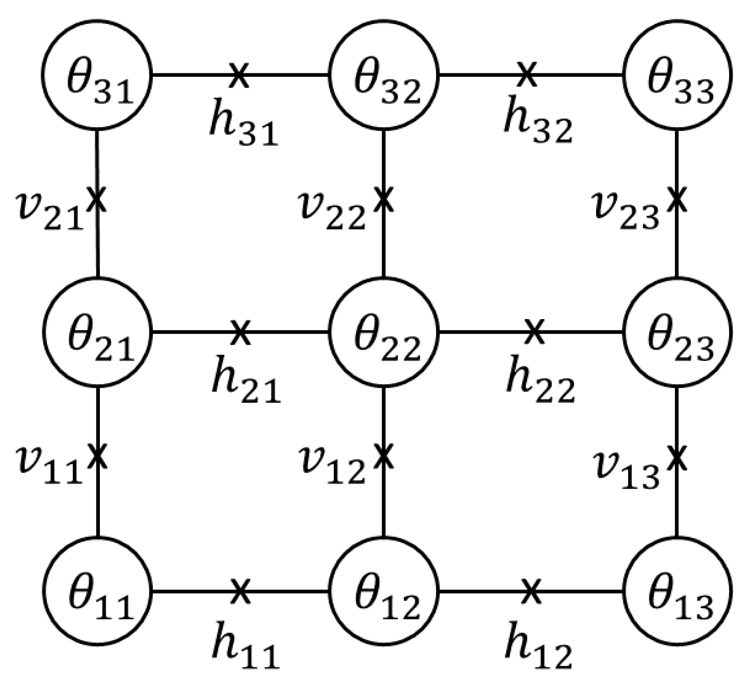
The ground states can be found by minimizing the Hamiltonian in Equation (
1) in terms of the superconducting phases
at each node. The Hamiltonian is defined in terms of the gauge invariant phase difference
, which is defined in terms of the superconducting phases
on the nodes in Equation (
2). Its principal value (pv) is taken in the interval
. The quantity
is defined as
. Here
is the magnetic vector potential. A perpendicular magnetic field is applied and a gauge is chosen such that
is zero for vertical junctions and
for horizontal junctions where
; i.e., the frustration factor defined as the magnetic flux treading a unit cell divided by the flux quantum. Furthermore,
y is the vertical coordinate of the junction. The Josephson Energy
is equal to
.
Equation (
3) is the quantization rule. The sum is taken along any closed path through the array,
is the magnetic flux through that path and
is the number of the Josephson vortices within the path. On a local minimum of
H in terms of
, the winding rules are automatically satisfied and the vortex configuration can be deduced from them.
For a given frustration, multiple local minima exist, and each local minimum corresponds to a configuration of Josephson vortices. The amount of local minima to the Hamiltonian for large systems grows strongly with the array size and becomes too large for a brute-force search. To find low energy states, simulated annealing is used on time dependent simulations. This is done with the RSJ model.
In the RSJ model [
22,
23], the current
through a junction between node
i and node
j is given by:
Here is the superconducting phase of node i. The current is split in three parts; the supercurrent through the Josephson element, the current through the parallel resistor and the Johnson noise generated in the parallel resistor. The Johnson noise has a correlation defined as .
The system of equations is obtained by enforcing Kirchhoff’s rules on each node. This results in a stochastic system of first order non-linear ordinary differential equations in time. This is solved numerically by applying a forward finite difference scheme in time. The stationary points of this system correspond to the minima of the Hamiltonian in Equations (
1)–(
3). The time discretization is worked out in
Appendix A. It is written in dimensionless quantities
,
. Then, at each timestep a linear system has to be solved of size
. This is done using the fast Poisson solver technique which is described in
Appendix B [
24]. Furthermore, the computation was done on a GPU for which this algorithm is well suited. The code was written in CUDA.
Simulations were done with , and . The time step was set to . The annealing procedure was done for each value of f separately. For , a run at a given f contains timesteps where is kept constant at for the first 20,000 steps and then linearly quenched to 0.
First, at a specific value of f, 100 runs are done in parallel with random initial conditions. With random is meant that the phase at each island is drawn from a uniform distribution between 0 and at . All runs end up in a state with a particular vortex configuration and energy. The second iteration again consists of 100 runs, but this time the phases at the final timestep of the first iteration were used as initial conditions. Now, out of the combined states at the end of the first iteration and at the end of the second iteration, the 100 best states with lowest energy were chosen as initial conditions for the third iteration. In total 50 iterations were done where the lowest energy states that were found up to that point are always taken as initial conditions for the subsequent iteration. This process was done for frustration factors between 0 and in steps of .
3. Results
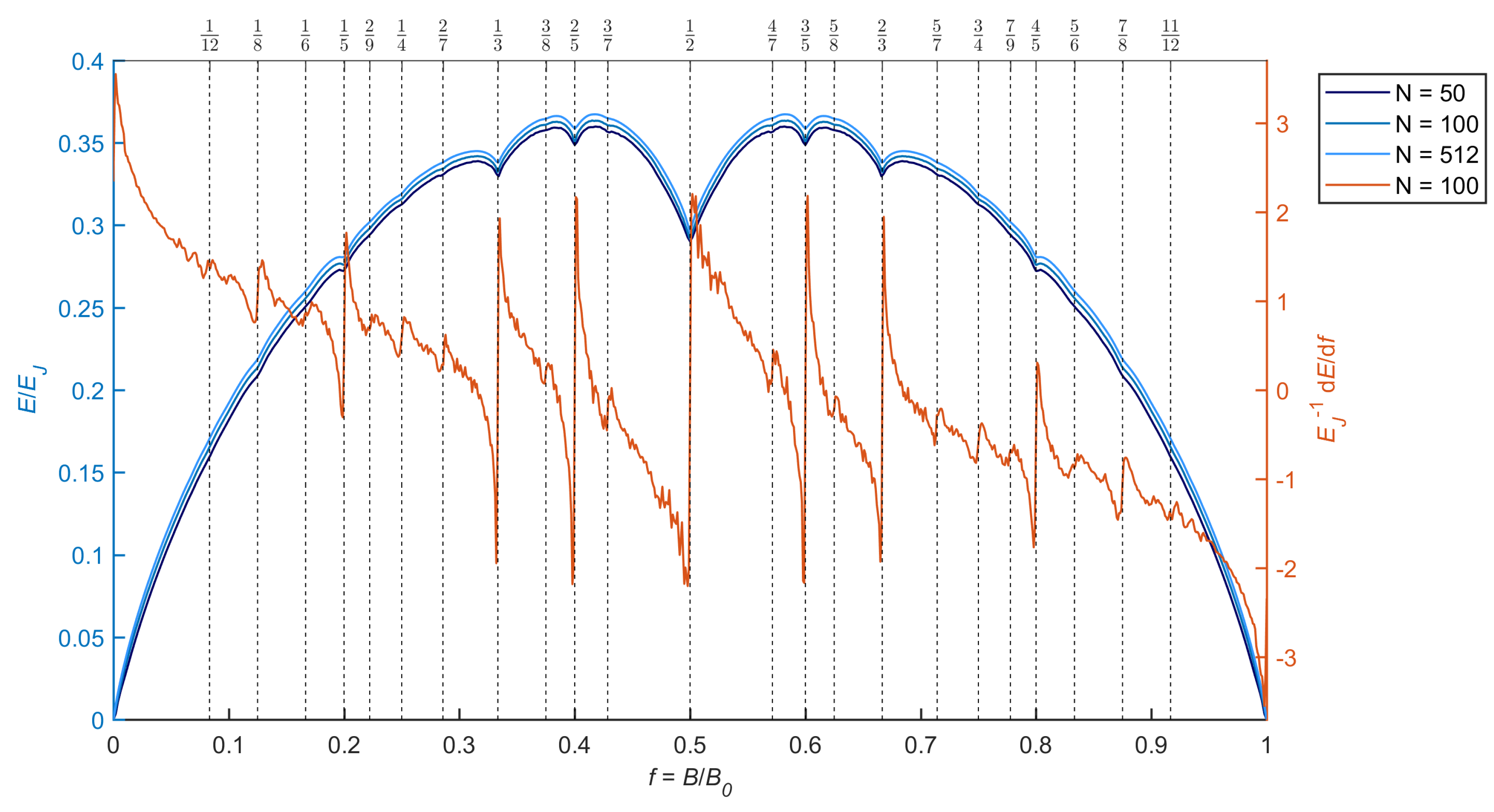
The obtained lowest energy states as a function of frustration factor are shown in
Figure 1. Simulations were only done for
and the data is reflected with respect to
, using the symmetry
,
,
. The lowest energy states form a smooth curve except at rational values of the frustration factor where the derivative
shows discontinuities in line with fractal behavior. The fractions at which the jumps in
exceed the noise level are highlighted. The derivative was computed numerically with a central difference scheme.
The curve appears to be continuous despite the fact that all points are independent problems starting from random initial conditions, confirming the continuity predicted by [
10]. This contradicts with the staircase state hypothesis. Furthermore, for a significant portion of the
f range between
and
with large
q, staircase states have significantly larger energy than the lowest energy states found with annealing. For these frustration factors the staircase states are likely not groundstates. Only slightly above and below
the energy for staircase states is lower than the lowest energy states found with annealing. The energy of the annealed states does still go down with longer annealing time and the energy difference is small enough that it is possible that for long enough annealing time the entire curve will be below or at the staircase state energy.
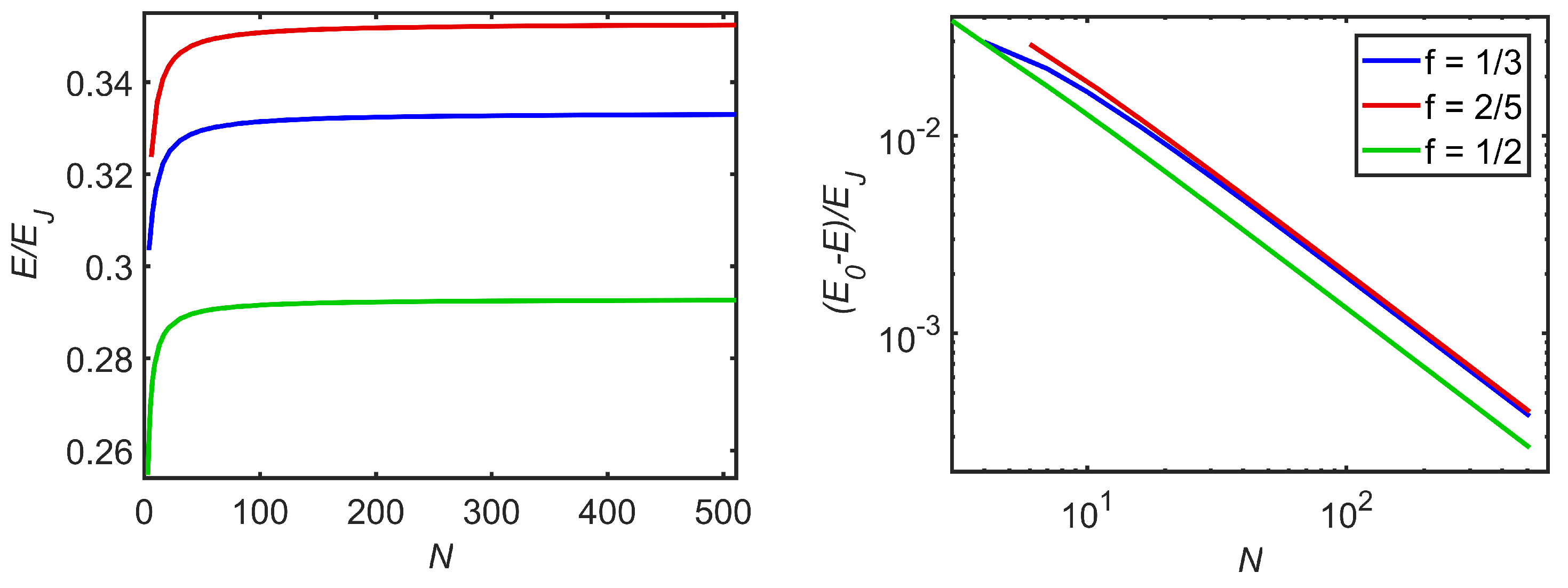
The lowest energy states depend on the size of the array. In
Figure 2 the energy is plotted as a function of array size for the small fractions
,
,
. Array sizes are taken to be integer multiples of
q and repetitions of the elementary tile are used as vortex patterns. For all these fractions the ground state energy converges to the limiting value as
for large
N.
,
,
were found. The limiting value
is known for these small fractions (it is
,
and
respectively). It was found that the junctions at the edge of the array have a lower Josephson Energy than junction in the center of the array. The width of this region is characterized by
, which is independent on array size but dependent on
f.
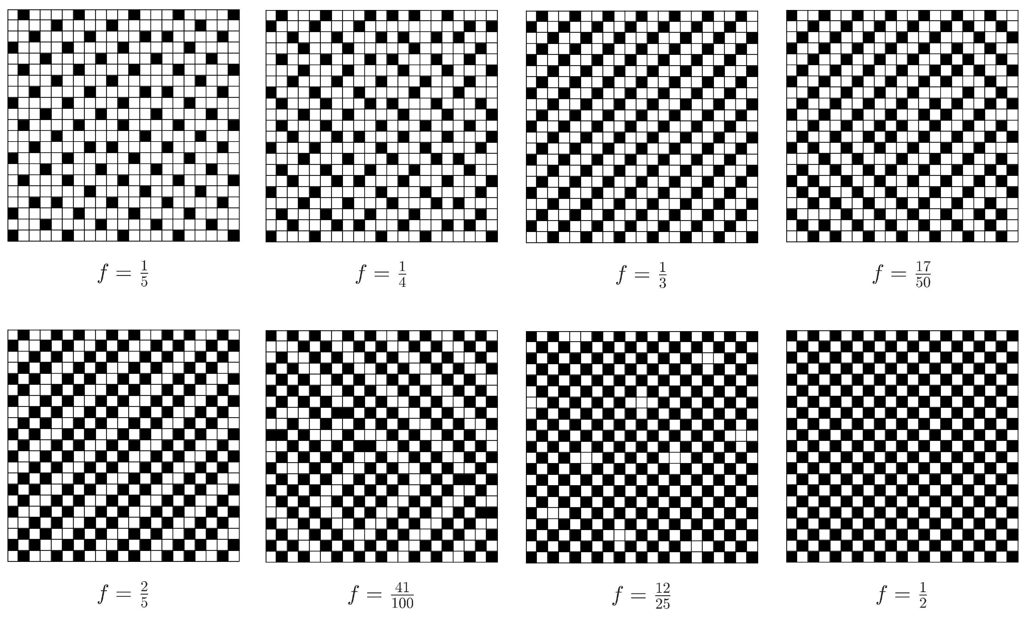
In
Figure 3 the vortex patterns on the center 21 by 21 tiles for some fractions are shown. Similar patterns have been observed in magnetic probe measurements on superconducting networks [
25,
26]. The patterns look as follows. For fractions
,
,
the vortex pattern that was found is equal to the tiled patterns corresponding to the ground state of infinitely large arrays. For other small fractions,
for example, this tiling is not retrieved but rather grains of the elementary tiling are present separated by grain boundaries. The number of grain boundaries gets smaller for longer annealing time, and it is plausible that these grain boundaries will completely disappear for sufficiently long annealing time.
For frustration factors close to small fractions
and
the vortex pattern looks to be a superposition of excitations on top of the vortex pattern corresponding to that fraction, which was also found in [
7]. It is known that in the regime
the vortex excitations are spaced far apart and can be treated as independent vortices which have logarithmic interaction and obey
[
27]. The derivative of the lowest energy curve has logarithmic singularities not just at
, but also at small fractions
where the graph obeys
. This suggests that for values of
f close to these small fractions, the vortex pattern is a superposition of base pattern plus a superlattice of defects.
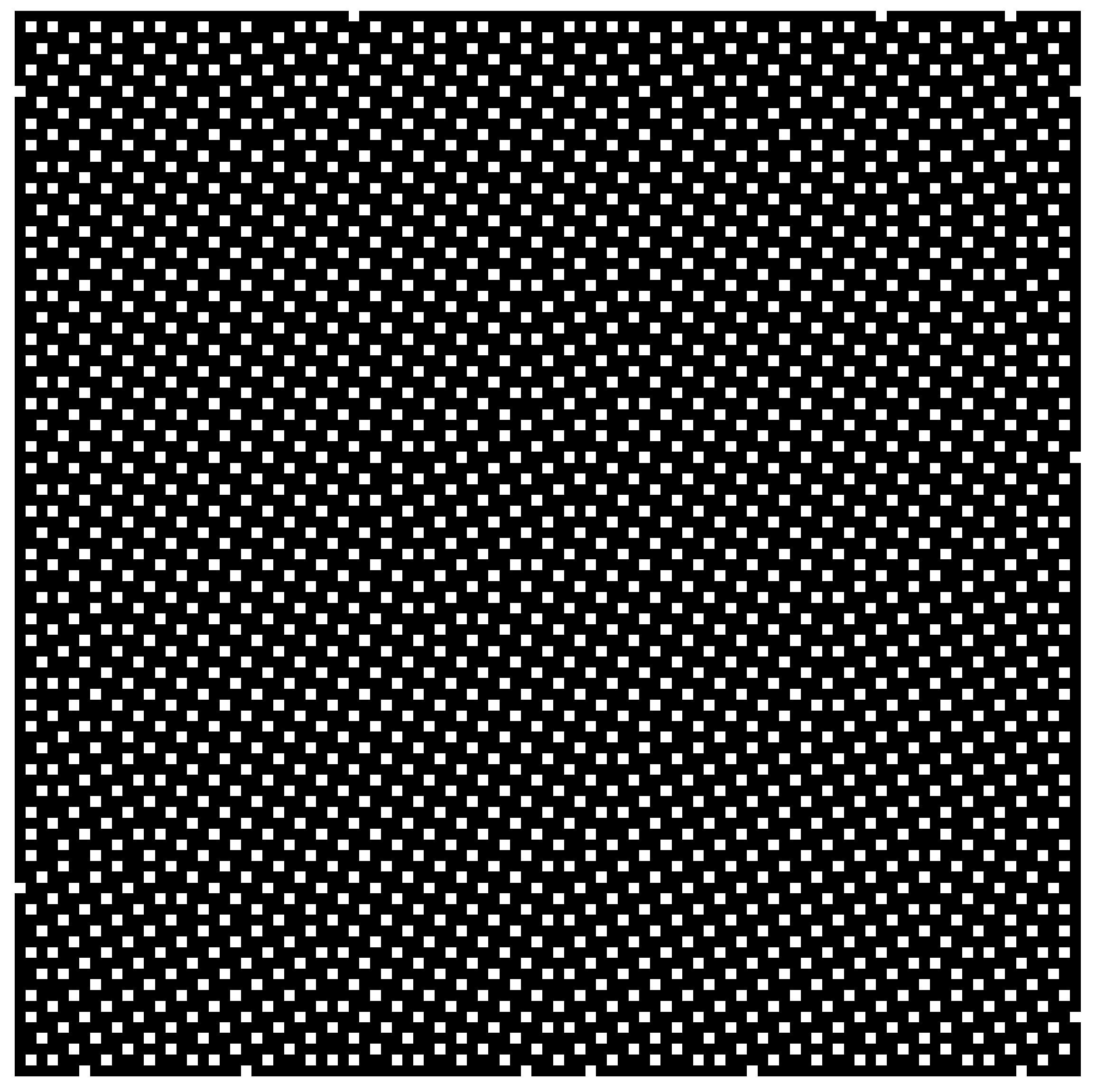
In
Figure 4, the full vortex configuration for
and
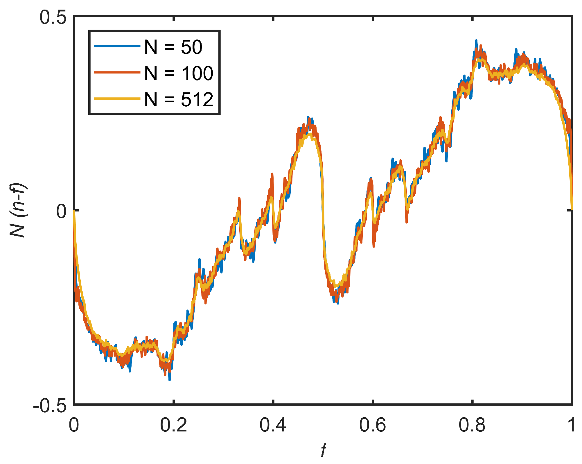
is shown. It is clear that vortices are missing at the edge. For an infinite array, the mean number of vortices is exactly equal to the frustration factor, but for a finite array it is allowed to deviate slightly. In
Figure 5 this difference times the array size is plotted as a function of frustration factor and array size. It appears that this follows a universal curve and the difference between the mean number of vortices
and
f scales as
just like the energy. This again implies that there is a field dependent depletion- or accumulation-width at the edge of the array, although this width is not the same as the energy relaxation width.
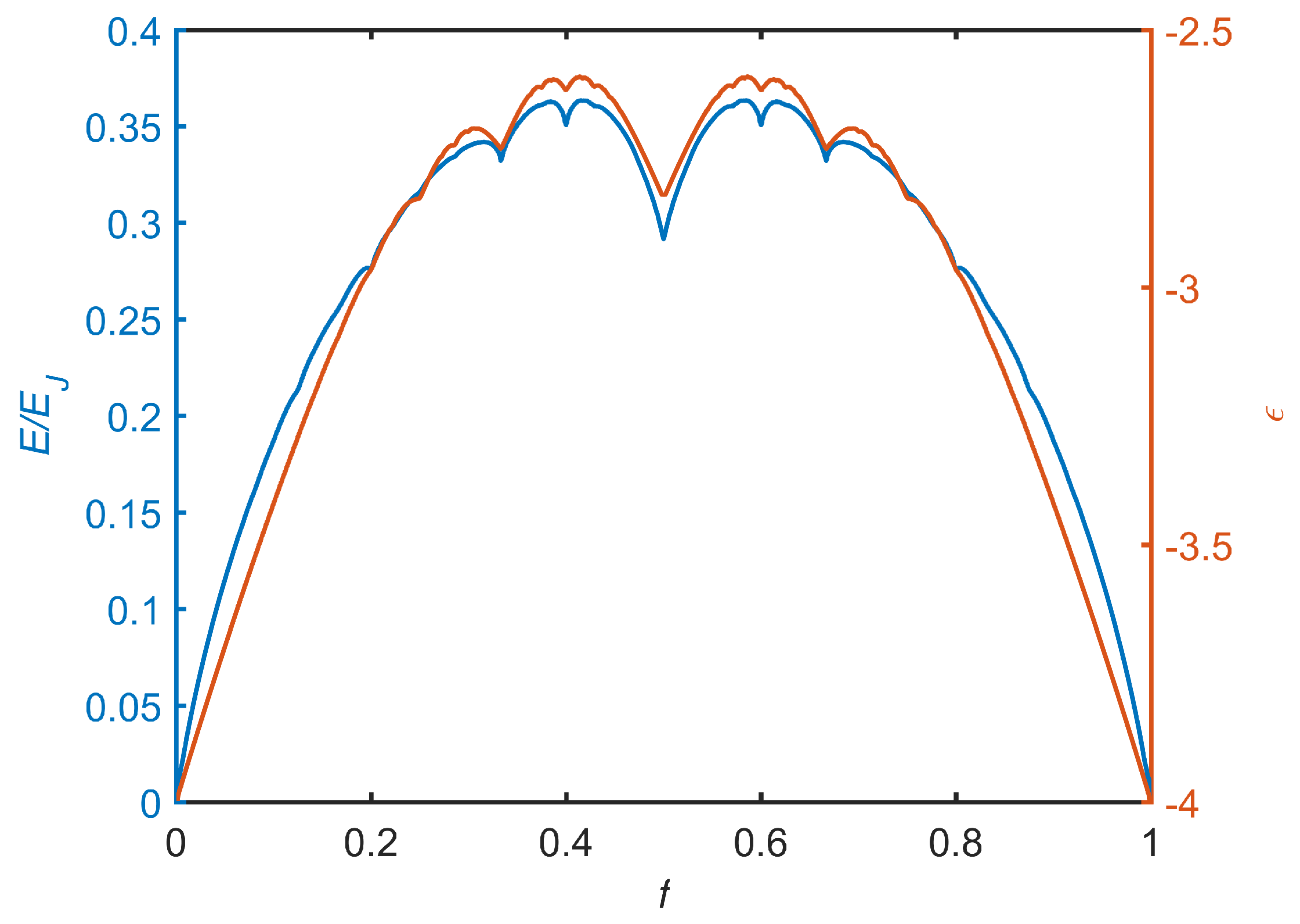
In
Figure 6 the lowest energy states of the frustrated XY model are compared to the lowest energy branch of the Hofstadter butterfly which is proportional to the
for superconducting networks as predicted by the linearized GL network equations [
18,
19,
20,
21]. The general shape of the curve is very similar and both show fractal behavior with apparent singularities at rational values of
f. However, these singularities seem of different type. In the frustrated XY model these singularities appear logarithmic, while in the Hofstadter butterfly the singularity is approached linearly from both sides. The similarity of these curves suggests there might be a connection between the ground state energy of JJAs and the
for superconducting networks.


