Abstract
Marine protected areas (MPAs) can allow some fish populations to rebuild within their borders in areas impacted by overfishing, but the effectiveness of reserves is highly dependent on how effectively fishing mortality is controlled, which in turn depends on the level of fishery management implementation. In Cuba’s Gardens of the Queen MPA, the largest in the Caribbean, a variety of fishery management measures have been implemented to ensure the social, economic, and political viability of protecting such a large area. Here, we evaluate the biological response, in terms of fish density and the biomass of commercially valuable and ecologically important reef fish species, to a spatial gradient of fishery management enforcement, in terms of fish density and biomass, of commercially valuable and ecologically important reef fish species. The enforcement gradient is characterized by the level of protection, fishing effort, patrolling effort, distance to the nearest fishing port, and fishing intensity. Fish density and biomass were estimated from visual scuba surveys. Areas with higher levels of enforcement support higher levels of average biomass (up to 1378 kg/ha) and density (up to 2367 indv./ha) of commercially important fishes in comparison to areas with very low or no enforcement (estimates of 757 kg/ha average biomass and 1090 indv./ha average density, respectively). These fish density and biomass levels can serve as proxies in the development of harvest control rules that adjust fishing pressure according to the ratio of fished density or biomass to unfished density or biomass, through the use of the MPA Density Ratio method.
Keywords:
stock assessment; data-limited; fisheries conservation; fishery-independent data; marine protected areas; MPA density ratio; fisheries policy; precautionary management Key Contribution:
A gradient in fishery management provides valuable estimates of multi-species fisheries health and reference points for harvest control rules using the MPA Density Ratio. The MPA Density Ratio method serves as an assessment option to support precautionary fisheries management in fisheries with little to no fishery-dependent data, such as the multi-species fishery around the Gardens of the Queen, Cuba.
1. Introduction
Overfishing continues to threaten the sustainability and resilience of fisheries, ecosystem functioning, livelihoods, and food and nutrition security worldwide [1,2,3]. This has led to the global consensus that these critical resources must be more effectively managed [4,5]. The elements of science-based fishery management associated with increased sustainability are relatively well-known [6,7] and important progress has been made, at least in some parts of the world [8].
The effective science-based management of fisheries delivers social and economic returns to fishery stakeholders, while also supporting ecosystem benefits that society values. In conventional fishery management systems, science-based management decisions are made on the basis of quantitative stock assessments [9]. Often, fisheries that lack sufficient information to conduct a conventional stock assessment are neither assessed nor managed with quantitative assessments, and many of these fisheries remain unassessed due to a lack of scientific capacity, data, or resources [10,11]. Thus, reliable assessment methods that are relatively fast, easy, use either fishery-dependent or -independent data streams, and require fewer data inputs than conventional methods would help increase precautionary fishery, presumably enhancing fishery performance [12].
Marine protected areas (MPAs) can be used to help rebuild and manage fish populations, especially in areas where conventional fisheries management is challenging to implement [13,14]. It has been demonstrated that well-managed and designed multiple-use MPAs represent a practical solution that balances both equitable fishery access and conservation goals, especially in situations in which the enforcement of fishery management is not achievable [15]. Currently, ~8.2% of the global ocean is officially designated or proposed to be part of an MPA [16]. While this is a valuable starting point for marine resource management, the potential benefits associated with the implementation of multi-use MPAs still have a long way to go [17]. MPAs vary in management intensity and effectiveness, with no-take/fully or highly protected areas covering about 2.9% (10,516,032 km2) of the ocean’s surface, implemented areas that are not fully or highly protected at 2.8% (726,644 km2), designated but unimplemented at 1.9% (6,791,811 km2) and proposed and unimplemented at 1.7% (6,250,593 km2). Though this estimate combines a wide range of MPA types with an equally wide range of objectives and expectations, of the 5.7% implemented MPAs, only 1.5% are implemented as highly protected and 1.4% as fully protected from fishing [16,18].
Despite the lack of fully protected areas in the ocean, it has been demonstrated that highly and moderately regulated areas exhibited a higher biomass and abundance of commercial fish species. Importantly, Zupan et al. identified that the effectiveness of moderately regulated areas can be enhanced by the presence of adjacent no-take marine reserves [19]. Also, there is increasing recognition of the utility of multi-use MPAs to deliver multiple goals [20]. These include an understanding of the local context, relative effectiveness, and enabling conditions of different levels of area-based management, all of which are essential for achieving positive biodiversity and fishery outcomes [20].
No-take marine reserves can also serve as a baseline for fishery assessment, aiding in the science-based management of these critical resources. Assessment methods that make use of data on the density, biomass, and size of fished targets inside and outside of the no-take reserves are an option to drive harvest control rules and regulate fishing mortality [21,22]. No-take reserves are also sometimes intended as “reference sites” to allow scientists to compare fished and unfished conditions [23]. For species that are harvested in areas around no-take marine reserves, ratios of the density or biomass outside to inside the reserves may be a useful indicator of the impact of fishing and aid in assessing the performance of fishery management efforts. Known as the MPA Density Ratio [21,22], this method can be applied to provide science-based guidance for precautionary fisheries management [7].
Countries are expanding marine protected area (MPA) networks to mitigate fisheries declines and support marine biodiversity, yet the impacts of various types of MPAs are poorly understood. The primary objective of this research is to demonstrate the influence of fishery management enforcement gradients within a multi-use MPA on targeted commercial fish species, while highlighting the MPA Density Ratio method [22] as a method to provide science-based precautionary fisheries management guidance [7] off of the southern coast of Cuba, which includes the Gardens of the Queens Marine Reserve (henceforth, Jardines de la Reina Marine Reserve, JRMR) and the addition of the national park (henceforth, “JRNP”).
2. Materials and Methods
2.1. Case Study
The Jardines de la Reina archipelago is approximately 135 km long and is made up of 661 cays and islands situated about 80 km off the coast of south-central Cuba, stretching from the cay of Bretón to Cabeza del Este (Figure 1). The archipelago supports a mosaic of mangrove islands, seagrass beds, and patch coral reefs, and is rich in fish, sharks, and other marine life [24]. Abiotic conditions such as sea surface temperature, water clarity, salinity, chronic wave exposure, and acute wave exposure are considered to be homogeneous across JRNP [25], and the coral reef condition and structural complexity (rugosity) are also homogenous [26]. The archipelago was heavily fished [24] until Resolution 562 was adopted by the national government in 1996 [27]; Resolution 562 established 950 km2 of the archipelago as a marine reserve.
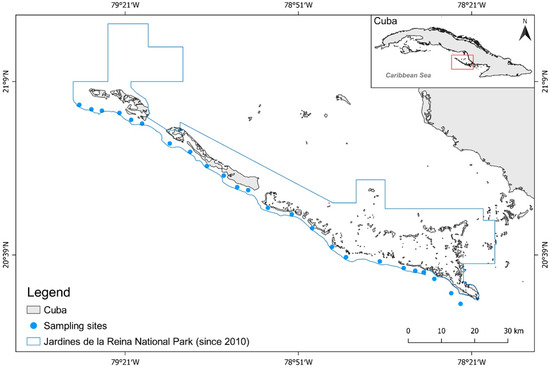
Figure 1.
Case study area, Gardens of the Queen National Park (JRNP), Cuba. Monitoring sites within the park (blue circles) and boundary of the national park (blue line).
Cuba defines an MPA as a marine or coastal portion of outstanding natural value devoted to the protection and maintenance of biodiversity, natural resources, and cultural values associated with the natural environment [28]. The country has established important management measures to protect its marine and terrestrial biota and is leading the designation of marine protected areas (MPAs) in the Caribbean region, as it includes approximately 25% of its insular shelf in an MPA designation [29]. Despite these measures, and similarly to many other regions in the world, most Cuban MPAs are not efficiently studied, monitored, enforced, or financed [29,30]. Cuban MPAs have been chosen for their high conservation value, and are often multi-use. For example, Resolution 562 made commercial fishing in JRMR subject to consent by the Directorate of Fishing Regulations and prohibited sport and recreational fishing unless authorized by a special permit.
The JRMR is in the heart of the archipelago, which comprises three cays. In 2010, under the Council of State Agreement 6803/2010 [31], 2170 km2 of the archipelago were set aside as protected, forming the Jardines de la Reina National Park. The JRNP with JRMR nested within the national park constitutes the largest contiguous marine reserve in Cuba and the Caribbean (ca. 2000 km2) [32]. Although the regulations establishing JRNP do not formally identify the park as having a no-take reserve, the center of the national park, JRMR, is recognized as a no-take reserve [27,31,33]. Fisheries regulations within the JRNP are considered well-enforced when compared to other Cuban regions and have an effective level of enforcement evidenced by the highest fish biomass in the Caribbean region [29,33]. The waters surrounding the archipelago (Gulf de Ana María and Gulf de Guacanayabo) are the primary fishing grounds for the Cuban commercial fishery, accounting for as much as 44% of the national total landings [34]. The finfish fishery in Cuba comprises 150 species, and the most common fishing gear are seine nets, gillnets, traps, bottom and surface longlines, and hook and line [34]. Set nets were banned in 2008 and trawls were banned in 2012. All of the coastal fisheries are managed within one of four management zones, and JRNP is within the south-east management zone.
2.2. Enforcement Gradient
As fishery regulations have evolved in Cuba, implementation and compliance, and therefore, the enforcement of regulations, have varied spatially and temporally, including within the JRMR and across the JRNP, resulting in an enforcement gradient [35]. The delineation of the different levels of fishery management enforcement across the JRNP is quantified by five parameters that have been measured since 2001: patrolling effort, fishing effort, fishing intensity, distance to the nearest fishing port, and protection level within the national park (Tables S1–S4). Collectively, these parameters aid in quantitatively defining the level of enforcement in the JRNP, which are defined here as enforcement parameters. Fishing intensity is defined by the type of fishery (e.g., recreational vs. commercial) and abundance of vessels, and fishing effort is a running average of the days at sea per year. Patrolling effort is the number of hours spent patrolling per week and is estimated through interviews with fishery inspectors/park rangers, and the minimum distance to the main fishing ports on the mainland from sampling sites reflects the ease of access to the park. Protection level is either yes or no, dependent upon the determination of whether a site is included in a legally protected area.
An initial assessment of the fishery management enforcement parameters in 2001 (Figure 2) qualitatively identified five enforcement zones ranging from None to Very Low, Low, Moderate, Moderate to High, and High levels of enforcement across JRNP [33] (Figure 3, Table 1). The None to Low-enforcement level represents sites within the region with high fishing intensity and effort, no protection, lower levels of patrolling efforts, and the closest to the fishing ports. The Low-enforcement level represents conditions similar to those within the None to Very Low-enforcement sites, except the sites are farther away from fishing ports. Meanwhile, the Moderate-enforcement level reflects sites with moderate fishing intensity and effort, protection, lower levels of patrolling efforts, and located far from fishing ports. The Moderate-High level of enforcement is like the Moderate-enforcement level, except it is farther from fishing ports. The High-enforcement level was identified to have the lowest fishing effort and intensity, being the farthest away from fishing ports, protection, and higher levels of patrolling effort. The initial assessment identified a spectrum of enforcement throughout the region that would become JRNP.
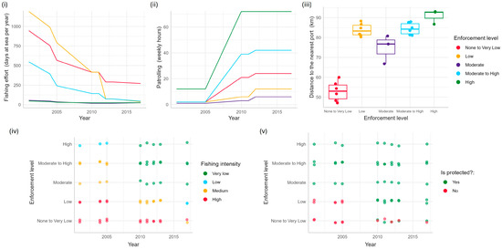
Figure 2.
The distribution of enforcement parameters over time and by enforcement level: None to Very Low (red), Low (orange), Moderate (purple), Moderate to High (blue), and High (green) for (i) fishing effort, (ii) patrolling effort, (iii) distance to the nearest fishing ports, (iv) fishing intensity, and (v) level of protection.
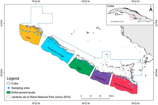
Figure 3.
Spatial distribution of the enforcement gradient in Gardens of the Queen, Cuba. Monitoring sites within the park (blue circles), boundary of the national park (blue line), and level of enforcement after the implementation in 2010.

Table 1.
Regression coefficients and model statistics for enforcement level analyses in JRNP.
Prior to the establishment of the JRNP in 2010, fishing intensity was thought to have been relatively high throughout the region. The fishing intensity was probably highest in the zones at the extreme ends of the region because the patrolling, reef protection, and enforcement levels were the lowest (e.g., zones of Low and None to Very Low enforcement). Levels of enforcement and compliance are both higher in the core of JRNP (High enforcement; the location of JRMR). Each enforcement parameter has increased in functionality over time (Figure 2), contributing to higher levels of fishery regulation implementation throughout JRNP, despite the continued existence of an enforcement gradient.
2.3. Field Sampling
Fishery-independent data of coral reef benthic habitat and fauna, using visual census underwater surveys on scuba, were collected on the fore reef (drop off and spur and groove) across the JRNP archipelago (2001–2017). Over time, the number of survey sites per expedition and within each zone has varied from 1 to 3, depending on the length of the expedition, resources available, and weather impacting safety and water clarity (i.e., <10 m). At the beginning of the surveys in 2001, the location of each transect was randomly selected and stratified across each monitoring site and revisited during each expedition. The visual survey method uses belt transects, with the size of the belt transect varying from 200 m2 (50 m × 4 m) to 8000 m2 (800 m × 10 m), and the number of sample units (transect or NSU) varying from 2 to 10 (Table S5), again depending on expedition length, resources, and weather conditions. Over the course of the study, all of the years surveyed have two NSUs, except for 2001 (NSU = 10) and 2017 (NSU = 6).
All observers have over five years of experience carrying out underwater visual censuses for fish in Cuban water. FPA has participated in all expeditions, and all observer data are compared to FPA throughout each expedition to detect errors or biases. To ensure that species identification, size estimation, belt transect size, and swim speed are standardized across observers, these metrics are always calibrated on the first day of each expedition. The fish size estimation is calibrated using fish models of several sizes; these data are not included in any analyses. All fish observations are assessed daily, and adjustments are made for consistency when needed. As of 2017, a total of 54 non-cryptic fish species have been monitored over 12 expeditions. Fish monitoring is focused on fish species that have at least part of the adult phase on coral reefs. Of those fish species, 28 are part of the fishery, and 13 have high importance in the fishery [32] (Table S4). The 13 species are as follows: Carangoides bartholomaei, Caranx latus, Caranx ruber, Epinephelus striatus, Lachnolaimus maximus, Lutjanus analis, Lutjanus cyanopterus, Lutjanus jocu, Mycteroperca bonaci, Mycteroperca tigris, Mycteroperca venenose, Scarus guacamaia, and Sphyraena barracuda. These 13 fish species represent pelagic and benthic species with diverse feeding habits (piscivorous, invertebrate predators, and herbivores), all targeted by numerous gear types. Each fish observed on the transect was identified to species and visually sized. All of the underwater visual surveys were conducted under the authority of the Centro de Inspección y Control Ambiental of Cuba, under multiple permits that span the study period. Each permit is listed by permit identification number/year (month, if applicable): 43/2001, 26/2004, 1/2005 (January), 13/2005 (April), 22/2005 (September), 35/2005 (December), 52/2010, 33/2011, 29/2012, 58/2013, and 81/2017.
2.4. Data Standardization
To account for variability in the sampling design, the fishery-independent observations of fish were standardized over time and space. Fish observations per transect are standardized to the area sampled (8000 m2) and estimated for both the density (number of individuals) and biomass (kilograms) per hectare; to account for the increased sampling in the 2005 monitoring [31,33], the observations were averaged for the year. The biomass of individual fishes was estimated using the length–weight conversion: W = aTLb, where parameters a and b are species-specific constants based on scientific studies, TL is total length (cm), and W is weight (g). Length–weight conversion parameters a and b were obtained from a comprehensive assessment of Cuba’s specific length–weight parameters [36,37] (Table S4). The estimated weight and the abundance for each species were used to estimate the average biomass by species and total biomass in each enforcement zone over time. Simultaneously, visual surveys across the archipelago collectively represented standardized habitats, depths, and oceanographic conditions. These data were rigorously checked for errors and integrated into a common database with a standardized structure.
2.5. Assessing and Defining the Enforcement Gradient across JRNP
To quantitatively assess the qualitatively pre-identified enforcement zones [35] and define the associated enforcement gradient based on evolving enforcement parameters over time, both exploratory and inferential analysis methods were utilized. Enforcement parameters encompassed a variety of data types, including binary, ordinal, and numeric variables. To assess if collinearity is present among the observed enforcement parameters, several methods were employed, including Pearson Correlation and Nonlinear Correlations (linear and nonlinear relationships), using nlcor 2.3 package [38]; Conditional Mutual Information (CMI), using the mpmi 0.43.2.1package [39] to quantify nonlinear direct relationships specifically among numeric variables; and Mann–Whitney U and Kruskal–Wallis Tests to assess associations between numeric and categorical variables, using the rstatix 0.7.2 package [40]. Subsequently, the ordinal 2023.12-4 package [41] was used to fit bivariate ordinal logistic regression models with a logit link function to evaluate the influence of each enforcement parameter (an ordinal variable) on the enforcement zones within the JRNP. A proportional odds assumption was also tested using the Brant test implemented in the gofcat 0.1.2 package [42] and the adjusted predictions from the models from the ggeffects 1.7.1 package [43].
Additionally, a non-metric multidimensional scaling (MDS) was used across JRNP’s monitoring sites to assess shifts in the enforcement gradient over time. The analysis used a Gower distance metric [44] to account for both categorical and numerical enforcement parameters, using the vegan 2.6-4 [45] and cluster 2.1.4 [46] packages. Each monitoring site’s annual data served as a unit of observation, and the aim was to capture non-parametric monotonic relationships between these units based on their dissimilarity in the enforcement parameters. To further examine the contribution of each enforcement parameter to the observed variability in clustering patterns among sites, years, and the level of enforcement, a non-linear PCA (nlPCA) was used with the Gifi 0.4-0 package [47]. All calculations were performed in R 4.3.2 [48].
2.6. Modeling Variability in Fish Biomass in JRNP
To compare spatial and temporal variations in fish biomass (both total and at the species-specific level) lognormal generalized linear mixed models (GLMM) were fitted using the lme4 1.1-35.5 package [49] and restricted maximum likelihood (REML) estimation, with enforcement as an ordered factor. When the response variables contained zeros, a small constant was added following the methods described in [50,51]. The models include fixed effects for the interaction between year and enforcement level. The random effects structure included a random intercept for sites nested within different enforcement levels, formulated as .
2.7. Impact of the Enforcement Gradient on Target Fish Species in JRNP
To evaluate the impact of varying enforcement levels of fishery management on targeted commercial finfish species across JRNP, we compared the average total density and biomass for each enforcement zone. Additionally, to evaluate the impact of the High-enforcement level on the fish biomass and density, we estimated the MPA Density Ratio (or MPA Ratio) for both total fish and species-specific biomass and density ratios over time in each enforcement level. The MPA Ratio is calculated as the average fish density or biomass found outside a no-take MPA to that within the MPA . This ratio is derived using stratified random sampling [22]. Typically, the density and biomass of fish within an MPA serve as proxies for unfished conditions, offering a benchmark for assessing stock status. The estimated ratios for density and biomass can in turn be compared to international reference points for the MPA Ratio to estimate stock status [21,22]. Though the regulations establishing JRNP do not identify the park as having a no-take reserve, the center of the national park, the High-enforcement zone, is recognized as a no-take area [27,31,33]. Since JRNP lacks a formally designated no-take reserve, we are instead interpreting the MPA Ratio as an indicator of the fish population response to different levels of enforcement to the High-enforcement zone and, therefore, levels of fishing pressure.
3. Results
3.1. Assessing and Defining the Enforcement Gradient across JRNP
The transition in the enforcement gradient in space and time is apparent in the clustering of enforcement zones over time, as shown in the nmMDS (Figure 4). The highest levels of enforcement occur in the High-enforcement and Moderate- to High-enforcement levels, with the other zones on a trajectory toward transitioning to the higher levels of enforcement (Figure S1). Specifically, the Low-enforcement zone transitioned to the higher levels of enforcement, developing characteristics of the early stages of the zones with higher enforcement, indicating dynamic progression (Figure 4). The enforcement zones with the lowest levels of enforcement (None to Very Low) cluster with the Moderate-enforcement zone over time. Post-2010, the least enforced eastern zone (None to Very Low-enforcement) diverges: the far east maintains negligible enforcement, while the west adopts Low enforcement. This divergence is clearer in a non-grouped plot (Figure S1). Both plots use the same data, but the first omits extra labels and includes a trajectory path for clarity.
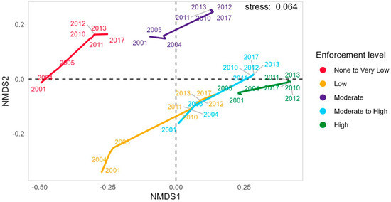
Figure 4.
Non-metric Multidimensional Scaling (nm-MDS) of enforcement parameters. Analysis of the evolution of zones through time, based on the variability of enforcement parameters.
The non-linear Principal Component Analysis explained 79% of the variability among the enforcement parameters over time. There is a strong positive correlation between the level of enforcement to patrolling hours, the minimum distance to fishing ports and the presence of coral reefs (Figure S2). Enforcement level and patrolling hours are inversely related to fishing effort and intensity, and fishing intensity is positively correlated with the absence of protective measures. The parameters of patrolling effort and distance to fishing ports are predominantly associated with enforcement zones that have High-enforcement levels in recent years. Conversely, fishing intensity correlates highly with None to Very Low-enforcement zones, indicating a shift away from high-exploitation practices over time. These findings point to heterogeneity in enforcement parameters, leading to distinct clustering patterns across enforcement zones and years (Figure 4, Figure S1).
The logistic regression analysis revealed that the protection status of a site significantly influences its enforcement level (Table 1). Specifically, sites lacking protection are less likely to exhibit higher enforcement levels than those that are protected (Figure S3A). There was a positive relationship between patrolling hours and enforcement levels (Table 1), with increasing patrolling hours being associated with higher levels of enforcement (Figure S3B). There was an inverse relationship between fishing effort and enforcement levels (Table 1), with higher fishing effort correlating with lower enforcement levels (Figure S3C). The model showed a strong negative link between fishing intensity and enforcement levels (Table 1); though the relationship was not uniformly linear, higher fishing intensity was consistently associated with lower enforcement levels, and the rate of change varied across different intensity levels (Figure S3D). The analysis indicated that the enforcement levels are influenced by the site’s distance from the nearest fishing ports (Table 1), sites situated further from ports tended to have higher enforcement levels (Figure S3E). However, these results came from a limited dataset of 24 observations, which could explain the wide confidence intervals.
3.2. Fish Biomass Variability in JRNP
The lognormal mixed model examining the influence of year and enforcement on total biomass explained 85% of the variance in total fish biomass (Table 2). There was a statistically positive effect of year on total fish biomass. Only the highest level of enforcement (High enforcement, p < 0.05) showed a significant association with changes in total fish biomass by year (year × High enforcement, p < 0.05). Furthermore, the interaction term (year × High enforcement) suggests that the effect of the High-enforcement level on total fish biomass decreases over time, resulting in similar estimates of total biomass across the enforcement levels at the end of the study.
Table 2.
GLMM fitted with restricted maximum likelihood (REML) estimation for total fish biomass.
In a species-specific analysis using GLMM, distinct trends emerged for the influence of year and enforcement level on fish biomass. Biomass for C. ruber, L. cyanopterus, L. maximus and E. striatus showed statistically significant increases over time (Table S6). Conversely, L. analis and C. latus experienced a decline in biomass over time, contrary to our preliminary findings. Notably, no species demonstrated a significant response solely due to varying levels of enforcement. However, two exceptional cases emerged: S. barracuda exhibited a statistically significant positive interaction between year and enforcement level, particularly year x High enforcement. For M. bonaci, the effect of year became significant only at the highest level of enforcement, with a significant interaction term of year x High enforcement. Conversely, L. jocu, S. guacamaia, M. tigris, C. bartholomaei, and M. venenosa did not exhibit statistically significant responses to either year or enforcement (Table S6). These species-specific outcomes supplement the broader analysis and offer nuanced perspectives on how year and enforcement levels may be affecting individual fish populations.
3.3. Impact of the Enforcement Gradient on Target Fish Species in JRNP
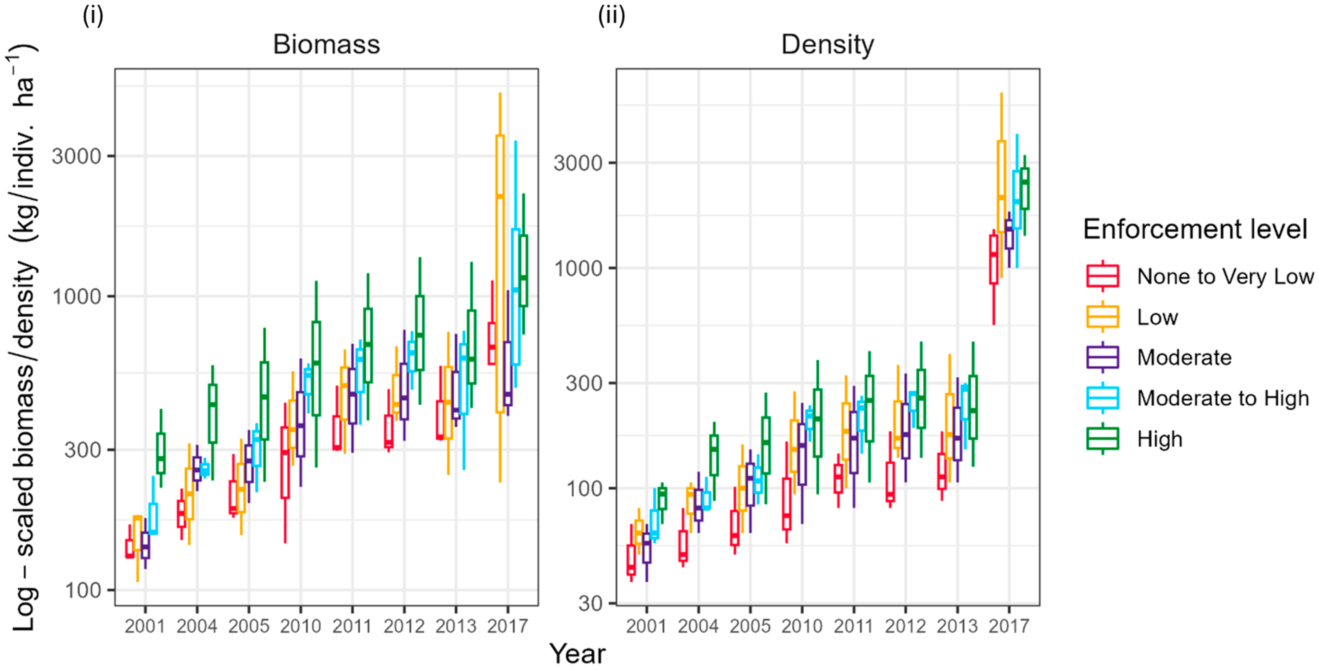
Establishing an enforcement gradient with varying levels of fishing pressure in space and time benefits fish biomass and the density of targeted fish. Across 42 survey sites, around 900 h were spent on visual survey counting and measuring 32,198 target fish (418,042 total fish observed) in 2001–2013 and in 2017. There were increases in the total fish density and biomass of targeted fish related to enforcement level, with the highest biomass and density of fish in the High-enforcement zone and the lowest biomass and density of fish in the None to Very Low-enforcement zone over time (Figure 5, Table S7). The Low-enforcement zone was estimated to have a similar or higher average total fish density and biomass than the Moderate-enforcement zone (Figure 5). This pattern is consistent throughout the study period. This was magnified in 2017 when the Low-enforcement zone had a higher average total density and biomass than each enforcement level. The overall trend is an increase in the average total fish biomass and density across each enforcement zone, but the increase in these parameters is most apparent in 2017. The Low-enforcement zone has the greatest magnitude of increase, with a twelve-fold increase in total fish density and a five-fold increase in total fish biomass (Table S7).

Figure 5.
Trends in total fish (i) biomass (kg/ha) and (ii) density (indiv/ha) across the enforcement gradient.
Within JRNP, the estimated total density ratios and total biomass ratios (Figure 6), and average ratio for each year (Table S8) exhibit an increasing trend over time and across the enforcement gradient when comparing each enforcement zone to the High-enforcement zone. The ratios of total fish density and total fish biomass in the None to Very Low-enforcement zone to that in the High-enforcement zone were 0.45 and 0.55 in 2017, respectively. Except for the average total fish density ratio in the None to Very Low-enforcement zone (0.45), the average total fish density ratios among the other levels of enforcement along the enforcement gradient (e.g., Low, Moderate, and Moderate-High) to the High-enforcement zone are all above 0.5 at the end of the study period, ranging from 0.56–1.21. The total density and biomass ratios for the Low-enforcement zone to the High-enforcement zone were above 1.0 at the end of the study period, indicating that the biomass and density of fish in the Low-enforcement zone have surpassed the High-enforcement zone. The average total fish biomass ratios among the other levels of enforcement along the enforcement gradient (e.g., None to Very Low, Low, Moderate, and Moderate-High) to the High-enforcement zone are all above 0.5, ranging from (0.55–1.02) over time (Figure 6).
Figure 6.
Comparison of the (i) density and (ii) biomass ratios across the enforcement gradient (None to Very Low, Low, Moderate, and Moderate-High) to the High-enforcement level, over time.
Density and biomass ratios were stable for some target species but not for others (Figures S4a–m and S5a–m). More specifically, the density and biomass ratios are stable between each enforcement zone (e.g., None to Very Low, Low, Moderate, and Moderate-High) to the High-enforcement zone for C. ruber, E. striatus, L. maximus, L. cyanopterus, M. bonaci, M. tigris, and M. venenose. On the other hand, S. guacamaia only showed stability along the enforcement gradient for the biomass ratios. L. analis was not observed in each enforcement zone throughout the study period, resulting in an incomplete dataset. There is an indication from the 2017 ratios that the density and biomass of L. analis did increase over time in each enforcement zone, with high density and biomass ratios in the None to Very Low, Low, Moderate, and Moderate-High enforcement zones. Otherwise, C. bartholomaei, C. latus, L. jocu, and S. barracuda showed little stability over time. Overall, there are few patterns present in both the density ratios and biomass ratios for individual fish species across the enforcement gradient and over time.
4. Discussion
Marine protected areas are widely advocated as a tool for the conservation of coral reef resources (e.g., [52]), with their effectiveness in conserving fish populations being largely dependent on the levels of compliance and enforcement, and the time since establishment [53,54]. In JRNP, the differential compliance and enforcement of fishery management measures has created an enforcement gradient across the multi-use MPA. This, in turn, has resulted in a gradient of fishing pressure, with lower fishing intensity and effort levels, and increases in the total fish density and biomass in the area considered a no-take marine reserve, the High-enforcement zone. On the other hand, in areas outside of the core of the marine reserve within JRNP, fishing intensity and enforcement decrease. Variability in compliance and consistent enforcement are among the most relevant issues concerning multi-use MPAs in providing either conservation or fisheries benefits [52]. Designing multi-use MPAs to have a gradient of enforcement might be a mechanism to balance social, economic, and ecological goals, given the difficulty in regulating compliance [15].
4.1. Enforcement Gradient Informs Fishery Status
The enforcement gradient identified in the JNRP is defined by both spatial and temporal shifts in the level of enforcement (Figure 3 and Figure 4). Though not statistically significant, the Low-enforcement zone exhibited a noticeable increase in the average total fish biomass and density over time compared to the Moderate-enforcement zone (Figure 5, Table 2). This phenomenon could be due to geographical factors, specifically the isolation of the Low-enforcement zone, as this zone is located in the west end of the National Park, which is farther from the nearest fishing port, in comparison to the Moderate-enforcement zone (Figure 2, Table 1) [54]. The nearest fishing port to the Low-Enforcement zone is across a large body of water, the Gulf of Ana Maria. The Gulf of Ana Maria also has many small islands close to the mainland, providing easy fishing near the mainland. Fishermen that cross the Gulf are likely fishing offshore, targeting large species outside the waters of JRNP [55], and not the fish in the Low-enforcement zone. Meanwhile, the Moderate-enforcement level is next to the None to Very-Low Enforcement zone and closer to the mainland, serving as the Low-enforcement level.
MPAs, together with other fishery science-based management tools, can help achieve broad fishery and biodiversity objectives [18,56,57]. Fish biomass and density levels and the average MPA Ratios (Table S8) across the enforcement gradient steadily increased over time; there was a large increase in fish biomass and density between 2013 and 2017 (Figure 5). Many species exhibit increases in abundance, shifts in length-frequency composition, and spawning stock biomass within MPA borders, which can enhance recruitment and spillover to adjacent areas [58,59]. Several studies have demonstrated the effectiveness of well-designed MPAs in managing fisheries in areas adjacent to the MPA [60], some with positive changes in reef fish biomass after a minimum of four years of protection [61,62,63,64]. The regional increase in fish populations is potentially connected to improving the enforcement of the marine reserve and implementing fisheries regulations, particularly the ban on set nets since 2008. Considering there were no monitoring expeditions between 2013 and 2017, we cannot assess the rate of change in fish populations over this period. Subsequent studies assessing fish biomass and abundance from 2018–2023 identified a similar increase in fish abundance and biomass across JRNP (35). Additionally, though not monitored, anecdotal evidence suggests a high recruitment success between 2013–2017, as a large school of jacks (Carangidae), including three of the species monitored in JRNP since 2001, has been observed throughout JRNP following the 2017 surveys. Considering that habitat, weather, sampling, and oceanographic conditions are similar across the region [24,25,26,27], we conclude that the enforcement of the marine reserve is one of the contributing factors to an increase in commercially targeted fish biomass and density across JRNP.
There are differences in variability in biomass and density ratio trends among the 13 individual species across the enforcement zones. Of the species showing stability in the biomass and density ratios through time, a few have a stable increase in the ratios, often in the Moderate-High and Low-enforcement zones (Figures S4 and S5). This includes species such as the groupers, snappers (except L. jocu), L. maximus, and S. guacamaia, each of these species are demonstrated to be positively impacted by the High-enforcement level in JRNP [33]. Large-bodied, slow-growing, and late-reproducing predators tend to be more abundant and larger in older and larger fully protected reserves [65,66,67] but not in all cases [68]. One factor consistently demonstrated to be positively correlated with fish biomass is the level of enforcement [69,70,71].
Of the species showing no stability in the biomass ratio over time, several species displayed a lot of variability between the enforcement zone over time. The lack of stability in the biomass and density ratios through time of these species is related to several factors: mobility, habitat structure, and species-specific fishing regulations. The jack species, C. bartholomaei, was primarily observed in JRNP in the natural size range of small to medium individuals (e.g., 10–40 cm fork length). These species school and are highly mobile [34], allowing for extensive movement along JRNP coral reefs, in turn making them susceptible to fishing pressure. Mobility can also result in high variability in encountering fish using visual census counts [72]. L. jocu occurs in large numbers in the None to Very Low-enforcement zone (no protection until 2010) and schools around sites with high structural complexity (numerous caves) in this zone, perhaps decreasing its vulnerability to fishing. Historically, the most prevalent gear used in this zone are set nets and fish trawls (Table S4); with these gear types, catching fish occurring in areas with high structural complexity without damaging gear would be difficult. S. barracuda is a ciguatoxic species, and fishing for barracuda is illegal in Cuba [73]. This regulation is considered to be well enforced nationwide, particularly in JRNP, where patrolling is frequent, perhaps explaining the observations of similar biomass levels across the enforcement gradient. C. latus showed no stability in the biomass ratios and no difference in biomass between each enforcement level at the end of the study. This species is highly mobile and forms large schools of large specimens (e.g., >50 cm fork length, [36]), allowing it to move extensively along the JRNP coral reef track and making it the most susceptible to fishing pressure, and the least responsive to zone-based protection measures.
Here we use the MPA or High-enforcement level to assess the status of fisheries and recommend control rules to implement management. Fish biomass and density levels across the enforcement gradient steadily increased over time (Figure 5), but the average total biomass varied markedly between the None to Very Low- and High-enforcement zones (range: 757.50–1378.01 kg/ha−1; Figure S3) at the end of the study period. The average total fish biomass (mean = 1292.77 kg/ha−1) across JRNP at the end of the study period is close to a previously identified mean Caribbean-wide unfished biomass (mean SD = 1306.55 kg/ha−1) level that is associated with low macroalgal cover, high proportions of invertivorous fishes, high levels of fish species richness, low urchin biomass, low ratios of macroalgal to coral cover, high proportions of herbivorous fishes, and high levels of coral cover in the Caribbean, or representative of a coral-dominated state [74]. Similar relationships were found for coral reefs in the Indian Ocean [75]. Based on the estimate of the average total fish biomass for JRNP, we concluded that the system is currently in a coral-dominated state and not at risk of state change. This interpretation is based on the result that the JRNP biomass is similar to an estimated average unfished biomass for the Caribbean; it is recommended to maintain a status quo of fishing and address any non-fishing threats [74].
4.2. Management Implications
After quantitatively assessing the enforcement gradient, it has become apparent that the levels of enforcement have evolved over time (Figure 4). It is recommended that the status of the Low-enforcement level be modified to Moderate, and the Moderate-enforcement level be changed to Low enforcement. By identifying how enforcement parameters interact and influence fish biomass and density within JRNP, managers can incorporate this knowledge to improve compliance and enforcement.
One of the advantages of marine reserves is that, unlike the traditional ‘single species’ approach, marine reserves offer an ecosystem-based approach to conservation and fisheries management [4] and as such might be a valuable tool in assessing the status and creating control rules in multi-species fisheries [76,77,78]. The potential of strategically expanding the existing global MPA network to increase future catch via spillover is still under investigation, but it is possible to generate more food annually than in a world with minimal protection [71,79], through better management.
Similarly, based on the MPA Density Ratio method, the ratios of total fish biomass (range 0.55–1.02) and total fish density (range 0.56–1.21) in JRNP indicate that this system may generally be at low risk for ecosystem change. For single fish stocks in temperate systems (typically with relatively low diversity and high productivity), biomass ratios near 0.5 are thought to be associated with maximum sustainable yield, ratios near 0.2 are thought to be associated with overfished status, and ratios between 0.2 and 0.5 are associated with pretty good yield (e.g., 80% of maximum sustainable yield, MSY) [22,56]. Coral reef stocks are highly diverse, and coral reef ecosystems are thought to be less productive than many temperate marine ecosystems; therefore, ratios in coral reefs associated with an overfished state may be somewhat higher than 0.2, the lower end of the pretty good yield range for temperate stocks [56]. Fishing down the average total fish biomass or density ratios near 0.3 in coral reefs will increase the risk of overfishing [74], resulting in lower long-term yields and a transition to macroalgal-dominated reefs. A ratio greater than 0.5 for single and multi-species coral reef fisheries has been identified as producing a pretty good yield in the Caribbean [74]. Ratios 0.25 < Biomass < 0.5 are a multi-species MSY indicator of impending ecosystem state change. At this point, a recommended precautionary control rule is to reduce fishing pressure. Even with a ratio > 0.5, a precautionary control rule in a data-limited fishery would be to continue monitoring the system and respond with lower fishing pressure if the ratio becomes <0.5 [74]. These precautionary control rules suggest that JRNP with an average density ratio of 0.68 (range 0.56–0.80 ± 0.08) and biomass ratio of 0.62 (range 0.51–0.92 ± 0.13) are above 0.5 throughout the study period, and the data-limited coral reef fisheries should continue to be monitored, but are considered sustainable.
Cuban finfish fisheries lack an ideal reference estimate of unfished biomass or density, though biomass and density in the High-enforcement zone may be good proxies due to the high level of enforcement of a relatively comprehensive set of regulations [80]. In this context, we recommend using a precautionary density and biomass ratios estimate of >0.5 as the MSY reference point. The multi-use JRNP, with a gradient of enforcement, provides a case study to combine the theoretical approach of the MPA Density Ratio method with the need to provide fishery access to achieve the social and economic goals of this fishery. The density ratio method provides a precautionary approach to articulate fishing pressure benchmarks intended to avoid risk and maintain the resilience of the ecosystem [7,11,12,81].
5. Conclusions
No-take marine reserves can provide valuable guidance for fishery management in the ratio of fished to unfished biomass or fish density as an indicator of stock status. However, enforced no-take reserves are relatively scarce, resulting in gradients in fishery management enforcement and, thus, fishing pressure, globally. We suggest enforcement gradients as a mechanism to balance multiple management goals and that, when coupled with High-enforcement zones that simulate no-take reserves, can be used to generate precautionary management guidance using density and biomass ratios. Furthermore, in countries with fewer resources to monitor MPAs, conservation goals can still be achieved by implementing a gradient of MPA protection and focusing enforcement efforts on the core no-take portion of the MPA system. We suggest that density and biomass ratio as a precautionary management tool [81], when used in combination with other assessment and management approaches, can greatly expand the number of fisheries that can be scientifically assessed and managed, which would be expected to improve fishery performance.
This study takes advantage of a diverse suite of fishery-independent monitoring efforts, thus maximizing the available data and certainty in designing adaptive, science-based management for JRNP [11,12,63]. The use of fishery-independent data and the MPA Density Ratio [22] along an enforcement gradient enables the assessment of fishery performance and precautionary management [7], even without dedicated no-take reserves.
Supplementary Materials
The following supporting information can be downloaded at: https://www.mdpi.com/article/10.3390/fishes9090355/s1, Figure S1: Non-metric Multidimensional Scaling (nm-MDS) of enforcement parameters post-2010 split in ‘None to Very Low’ enforcement zone, highlighting divergence in eastern sites; Figure S2: Non-linear Principal Components Analysis (nlPCA) explains 79% of the variability in the enforcement parameters. Analysis of the evolution of zones through time, based on the variability of enforcement parameters; Figure S3: Predicted enforcement levels based on (A) protection status, (B) patrolling effort, (C) fishing effort, (D) fishing effort, and (E) distance to the nearest port, as determined by ordinal logistic regression analysis; Figure S4: Density ratio analysis for each species along an enforcement gradient over time. Density ratio represents the average density in the None to Very Low-, Low-, Moderate-, Moderate-High-enforcement zone to the High-enforcement zone for each species over time: (a) Carangoides bartholomaei, (b) Caranx latus, (c) Caranx ruber, (d) Epinephelus striatus, (e) Lachnolaimus maximus, (f) Lutjanus analis, (g) Lutjanus cyanopterus, (h) Lutjanus jocu, (i) Mycteroperca bonaci, (j) Mycteroperca tigris, (k) Mycteroperca venenosa, (l) Scarus guacamaia, and (m) Sphyraena barracuda; Figure S5. Biomass ratio analysis for each species along an enforcement gradient over time. Biomass ratio represents the average biomass in the None to Very Low-, Low-, Moderate-, Moderate-High-enforcement zone to the High-enforcement zone for each species over time: (a) Carangoides bartholomaei, (b) Caranx latus, (c) Caranx ruber, (d) Epinephelus striatus, (e) Lachnolaimus maximus, (f) Lutjanus analis, (g) Lutjanus cyanopterus, (h) Lutjanus jocu, (i) Mycteroperca bonaci, (j) Mycteroperca tigris, (k) Mycteroperca venenosa, (l) Scarus guacamaia, and (m) Sphyraena barracuda. Management reference point of 0.5 identified with a dash line; Table S1: Description of the enforcement parameters; Table S2: Frequency of patrolling by fisheries inspectors in each monitoring zone of the Gardens of the Queen from 2001 through 2017: patrolling at sea on a daily basis (1); patrolling at sea on a weekly basis (2); patrolling at sea on a monthly basis (3); and patrolling at sea on a frequency lower than monthly (4). The average patrolling hours for 2005 are represented in this table, as 2005 had four expeditions (January 2005, April 2005, September 2005, and December 2005); Table S3: Transformation of enforcement parameters; Table S4: Description of biological parameters, a summary of fishery-independent monitoring and fishing gear used to catch each species; scientific name (SN), length–weight conversion parameters (a and b), common name (CN), maximum size (MS) in JRNP fishery-independent monitoring, frequency (%) (F), pelagic (P), and benthic (B); feeding habit (FH): piscivorous (P), invertebrate predators (I), or herbivorous (H); gear: gill net (GN), set net (SN), finfish trawl (FT), longline (LO), hook and line (HL), spearfishing (SP), and trap (TP). Pelagic/benthic and feeding habits information were taken from Claro (1994); Table S5: Spatial and temporal variability in field sampling for each zone, replicates per year, sample unit size on m2 (SUS), and number of sample units (NSN). The sampling shaded in gray represents the sampling regime in 2005 (January 2005, April 2005, September 2005, and December 2005); the four expeditions were averaged for 2005; Table S6: GLMM fitted with restricted maximum likelihood (REML) estimation for fish biomass: (a) Carangoides bartholomaei, (b) Caranx latus, (c) Caranx ruber, (d) Epinephelus striatus, (e) Lachnolaimus maximus, (f) Lutjanus analis, (g) Lutjanus cyanopterus, (h) Lutjanus jocu, (i) Mycteroperca bonaci, (j) Mycteroperca tigris, (k) Mycteroperca venenosa, (l) Scarus guacamaia, and (m) Sphyraena barracuda biomass; Table S7: Average total fish density and biomass in each enforcement zone by year; Table S8: Average total fish density and biomass ratios + one standard deviation (SD) for each year, comparing enforcement levels to the High-enforcement level.
Author Contributions
Conceptualization, K.A.K., F.P.-A. and T.F.-M.; methodology, K.A.K., F.P.-A., T.F.-M. and Y.O.-E.; formal analysis, K.A.K. and Y.O.-E.; data curation, F.P.-A. and Y.O.-E.; writing—original draft preparation, K.A.K.; writing—review and editing, K.A.K., F.P.-A., T.F.-M. and Y.O.-E.; visualization, Y.O.-E. All authors have read and agreed to the published version of the manuscript.
Funding
This research received no external funding.
Institutional Review Board Statement
Not applicable.
Informed Consent Statement
Not applicable.
Data Availability Statement
Data are contained within the article and supplementary materials.
Acknowledgments
All of the authors would like to thank Valerie Miller and Eduardo Boné-Morón for logistical and communication support. Additionally, we would like to thank Pete Raimondi, Rick Starr, and two anonymous reviewers for input and critical reviewers of the manuscript. F.P.A., T.F.-M., and Y.O.E. would like to thank Avalon-Marlin for the logistical support. They would also like to thank the many institutions and associated personnel of cooperative research projects that have advanced coral reef research and conservation in Jardines de la Reina, including Project “Atlantic and Gulf Rapid Reef Assessement”, Project “Archipiélagos del Sur”, Centro de Investigaciones de Ecosistemas Costeros, Centro de Investigaciones Marinas de la Universidad de la Habana, Instituto de Oceanología/Instituto de Ciencias del Mar, Centro Nacional de Areas Protegidas, Empresa para la Protección de la Flora y la Fauna, and Centro de Investigaciones Pesqueras. We appreciate the work of anonymous reviewers for their critical comments that have improved this paper.
Conflicts of Interest
The authors have declared that no competing interests exist.
References
- Barange, M.; Bahri, T.; Beveridge, M.C.M.; Cochrane, K.L.; Funge-Smith, S.; Poulain, F. (Eds.) Impacts of Climate Change on Fisheries and Aquaculture: Synthesis of Current Knowledge, Adaptation and Mitigation Options; FAO Fisheries and Aquaculture Technical Paper No. 627; FAO: Rome, Italy, 2018; 628p. [Google Scholar]
- FAO. The State of World Fisheries and Aquaculture—Meeting the Sustainable Development Goals (No. CC BY-NC-SA 3.0 IGO). 2018. Available online: https://www.fao.org/family-farming/detail/en/c/1145050/ (accessed on 1 April 2024).
- Bennett, A.; Patil, P.; Kleisner, K.; Rader, D.; Virdin, J.; Basurto, X. Contribution of Fisheries to Food and Nutrition Security: Current Knowledge, Policy, and Research; NI Report 18-02; Duke University: Durham, NC, USA, 2018; Available online: https://wfpc.sanford.duke.edu/reports/contribution-fisheries-food-nutrition-security-current-knowledge-policy-and-research/ (accessed on 1 April 2024).
- Lubchenco, J.; Palumbi, S.R.; Gaines, S.D.; Andelman, S. Plugging a hole in the ocean: The emerging science of marine reserves. Ecol. Appl. 2003, 13, S3–S7. [Google Scholar] [CrossRef]
- Lubchenco, J.; Gaines, S.D. A new narrative for ocean science. Science 2019, 364, 911. [Google Scholar] [CrossRef] [PubMed]
- Worm, B.; Hilborn, R.; Baum, J.K.; Branch, T.A.; Collie, J.S.; Costello, C.; Fogarty, M.J.; Fulton, E.A.; Hutchings, J.A.; Jennings, S.; et al. Rebuilding global fisheries. Science 2009, 325, 578–585. [Google Scholar] [CrossRef] [PubMed]
- Cochrane, K.L.; Andrew, N.L.; Parma, A.M. Primary fisheries management: A minimum requirement for provision of sustainable human benefits in small-scale fisheries. Fish Fish. 2011, 12, 275–288. [Google Scholar] [CrossRef]
- Hilborn, R.; Amoroso, R.O.; Anderson, C.M.; Baum, J.K.; Branch, T.A.; Costello, C.; de Moor, C.L.; Faraj, A.; Hively, D.; Jensen, O.P.; et al. Effective fisheries management instrumental in improving fish stock status. Proc. Natl. Acad. Sci. USA 2020, 117, 2218–2224. [Google Scholar] [CrossRef]
- Mace, P.M. Relationships between common biological reference points used as thresholds and targets of fisheries management strategies. Can. J. Fish. Aquat. Sci. 1994, 51, 110–122. [Google Scholar] [CrossRef]
- Dowling, N.A.; Wilson, J.R.; Cope, J.M.; Dougherty, D.T.; Lomonico, S.; Revenga, C.; Snouffer, B.J.; Salinas, N.G.; Torres-Cañete, F.; Chick, R.C.; et al. The FishPath approach for fisheries management in a data- and capacity-limited world. Fish Fish. 2023, 24, 212–230. [Google Scholar] [CrossRef]
- Karr, K.A.; Fujita, R.; Carcamo, R.; Epstein, L.; Foley, J.R.; Fraire-Cervantes, J.A.; Gongora, M.; Gonzalez-Cuellar, O.T.; Granados-Dieseldorff, P.; Guirjen, J.; et al. Integrating Science-Based Co-Management, Partnerships, Participatory Processes and Stewardship Incentives to Improve the Performance of Small-Scale Fisheries. Front. Mar. Sci. 2017, 4, 345. [Google Scholar] [CrossRef]
- Fujita, R.; Karr, K.; Battista, W.; Rader, D. A Framework for Developing Scientific Management Guidance for Data-Limited Fisheries. In Proceedings of the 66th Gulf and Caribbean Fisheries Institute, Corpus Christi, TX, USA, 4–8 November 2013; p. 66. [Google Scholar]
- Ovando, D.; Caselle, J.E.; Costello, C.; Deschenes, O.; Gaines, S.D.; Hilborn, R.; Liu, O. Assessing the population-level conservation effects of marine protected areas. Conserv. Biol. 2021, 35, 1861–1870. [Google Scholar] [CrossRef]
- Wilson, J.R.; Bradley, D.; Phipps, K.; Gleason, M.G. Beyond protection: Fisheries co-benefits of no-take marine reserves. Mar. Policy 2020, 122, 104224. [Google Scholar] [CrossRef]
- Gill, D.A.; Lester, S.E.; Free, C.M.; Pfaff, A.; Iversen, E.; Reich, B.J.; Yang, S.; Ahmadia, G.; Andradi-Brown, D.A.; Darling, E.S.; et al. A diverse portfolio of marine protected areas can better advance global conservation and equity. Proc. Natl. Acad. Sci. USA 2024, 121, e2313205121. [Google Scholar] [CrossRef]
- MPA Atlas. 2023. Available online: https://mpatlas.org/ (accessed on 13 January 2024).
- Turnbull, J.W.; Johnston, E.L.; Clark, G.F. Evaluating the social and ecological effectiveness of partially protected marine areas. Conserv. Biol. 2021, 35, 921–932. [Google Scholar] [CrossRef] [PubMed]
- Sala, E.; Lubchenco, J.; Grorud-Colvert, K.; Novelli, C.; Roberts, C.; Sumaila, U.R. Assessing real progress towards effective ocean protection. Mar Policy 2018, 91, 11–13. [Google Scholar] [CrossRef]
- Zupan, M.; Fragkopoulou, E.; Claudet, J.; Erzini, K.; Horta e Costa, B.; Gonçalves, E.J. Marine partially protected areas: Drivers of ecological effectiveness. Front. Ecol. Environ. 2018, 16, 381–387. [Google Scholar] [CrossRef]
- Ban, N.C.; Darling, E.S.; Gurney, G.G.; Friedman, W.; Jupiter, S.D.; Lestari, W.P.; Yulianto, I.; Pardede, S.; Tarigan, S.A.R.; Prihatiningsih, P.; et al. Effects of management objectives and rules on marine conservation outcomes. Conserv. Biol. 2023, 37, e14156. [Google Scholar] [CrossRef]
- Babcock, E.A.; MacCall, A.D. How useful is the ratio of fish density outside versus inside no-take marine reserves as a metric for fishery management control rules? Can. J. Fish. Aquat. Sci. 2014, 68, 343–359. [Google Scholar] [CrossRef]
- McGilliard, C.R.; Hilborn, R.; MacCall, A.; Punt, A.E.; Field, J.C. Can information from marine protected areas be used to inform control-rule-based management of small-scale, data-poor stocks? ICES J. Mar. Sci. 2011, 68, 201–211. [Google Scholar] [CrossRef]
- Bohnsack, J.A. Incorporating no-take marine reserves into precautionary management and stock assessment. In Proceedings of the 5th National NMFS Stock Assessment Workshop, Key Largo, FL, USA, 24–26 February 1998; pp. 8–16. Available online: www.st.nmfs.noaa.gov/StockAssessment/workshop_documents/nsaw5/bohnsack.pdf (accessed on 1 March 2023).
- Claro, R.; Sadovy de Mitchenson, I.; Lindeman, K.C.; García–Cagide, A. Historical analysis of Cuban commercial fishing effort and the effects of management interventions on important reef fishes from 1960–2005. Fish Res. 2009, 99, 7–16. [Google Scholar] [CrossRef]
- Chollett, I.; Mumby, P.J.; Muller–Karger, F.E.; Chuanmin, H. Physical environments of the Caribbean Sea. Limnol. Oceanogr. 2012, 57, 1233–1244. [Google Scholar] [CrossRef]
- Pina–Amargós, F.; Hernández–Fernández, L.; Clero–Alonso, L.; González–Sansón, G. Características de hábitats coralinos en Jardines de la Reina. Cuba Rev. Investig. Mar. 2008, 29, 225–237. [Google Scholar]
- Ministerio de la Industria Pesquera. Resolución N° 562/96—Declarar Como Zona Bajo Régimen Especial de uso y Protección las Aguas Marítimas Comprendidas en los Tramos Delimitados por Coordenadas Geográficas Específicas. Havana, Cuba, 1996. Available online: https://www.gacetaoficial.gob.cu/es/gaceta-oficial-no046-ordinaria-de-1996 (accessed on 5 September 2024).
- CNAP (Centro Nacional de Áreas Protegidas). Plan del Sistema Nacional de Áreas Protegidas de Cuba: Período 2014–2020; Ministerio de Ciencia, Tecnología y Medio Ambiente: Havana, Cuba, 2013; p. 336. [Google Scholar]
- Perera-Valderrama, S.; Hernández-Ávila, A.; González-Méndez, J.; Moreno-Martínez, O.; Cobián-Roja, S.D.; Ferro-Azcona, H.; Aragón, H.C.; Alcolado, P.M.; Pina-Amargós, F.; Hernández González, Z. Marine protected areas in Cuba. Bull. Mar. Sci. 2018, 94, 423–442. [Google Scholar] [CrossRef]
- Angulo-Valdés, J.A.; Navarro-Martínez, Z.; López-Castañeda, L.; Frazer, T.; Adams, A.J. Collaborating on a new vision for Cuba’s coastal fisheries. Bonefish Tarpon Trust J. 2017, 40–44. Available online: https://www.bonefishtarpontrust.org/wp-content/uploads/2018/12/2017-journal-fall.pdf (accessed on 5 September 2024).
- Hernández-Fernández, L.; Bustamante López, C.; Dulce Sotolongo, L.B.; Pina Amargós, F.; Figueredo Martín, T. Influencia del Gradiente de Protección Sobre el Estado de las Comunidades de Corales y Algas Coralinas Costrosas en el Parque Nacional Jardines de la Reina, Cuba. J. Mar. Res. 2018, 38, 83–99. Available online: https://revistas.uh.cu/rim/article/view/4212 (accessed on 5 September 2024).
- Appeldoorn, R.S.; Lindeman, K.C.A. Caribbean-Wide Survey of Marine Reserves: Spatial Coverage and Attributes of Effectiveness. Gulf Cari Res. 2003, 14, 139–154. [Google Scholar] [CrossRef]
- Pina-Amargós, F.; González–Sansón, G.; Martín–Blanco, F.; Valdivia, A. Evidence for protection of targeted reef fish on the largest marine reserve in the Caribbean. PeerJ 2014, 2, e274. [Google Scholar] [CrossRef]
- Puga, R.; Valle, S.; Kritzer, J.P.; Delgado, G.; Estela de León, M.; Giménez, E.; Ramos, I.; Moreno, O.; Karr, K.A. Vulnerability of nearshore tropical finfish in Cuba: Implications for scientific and management planning. Bull. Mar. Sci. 2018, 94, 377–392. [Google Scholar] [CrossRef]
- Pina-Amargós, F.; González-Díaz, P.; González-Sansón, G.; Aguilar-Betancourt, C.; Rodríguez-Cueto, Y.; Olivera-Espinosa, Y.; Figueredo-Martín, T.; Rey-Villiers, N.; Arias Barreto, R.; Cobián-Rojas, D.; et al. Chapter 15: Status of Cuban Coral Reefs. In Coral Reefs of Cuba, Coral Reefs of the World; Zlatarski, V., Reed, J.K., Pomponi, S.A., Brooks, S., Farrington, S., Eds.; Springer Nature: Cham, Switzerland, 2024; Volume 18, pp. 283–308. [Google Scholar] [CrossRef]
- Claro, R. (Ed.) Ecología de los Peces Marinos de Cuba; Instituto de Oceanología Academia de Ciencias de Cuba: Quintana Roo, México, 1994; p. 525. [Google Scholar]
- Froese, R.; Pauly, D. (Eds.) FishBase. 2013. Available online: https://www.fishbase.org (accessed on 5 September 2024).
- Ranjan, C.; Najari, V. nlcor: Nonlinear Correlation. Res. Gate 2019. [Google Scholar] [CrossRef]
- Pardy, C. mpmi: Mixed-Pair Mutual Information Estimators, R Package Version 0.43.2.1. 2023. Available online: https://r-forge.r-project.org/projects/mpmi/ (accessed on 5 September 2024).
- Kassambara, A. rstatix: Pipe-Friendly Framework for Basic Statistical Tests, R Package Version 0.7.2. 2023. Available online: https://cran.r-project.org/web/packages/rstatix/index.html (accessed on 5 September 2024).
- Christensen, R. Ordinal-Regression Models for Ordinal Data, R Package Version 2023.12-4. 2023. Available online: https://cran.r-project.org/web/packages/ordinal/ordinal.pdf (accessed on 5 September 2024).
- Ugba, E. gofcat: Goodness-of-Fit Measures for Categorical Response Models, R Package Version 0.1.2. 2023. Available online: https://cran.r-project.org/web/packages/gofcat/gofcat.pdf (accessed on 5 September 2024).
- Lüdecke, D. ggeffects: Tidy Data Frames of Marginal Effects from Regression Models. J. Open Source Softw. 2018, 3, 772. [Google Scholar] [CrossRef]
- Gower, J.C. A general coefficient of similarity and some of its properties. Biometrics 1971, 27, 623–637. [Google Scholar] [CrossRef]
- Oksanen, J.; Simpson, G.L.; Blanchet, F.G.; Kindt, R.; Legendre, P.; Minchin, P.R.; O’Hara, R.B.; Simpson, G.L.; Sólymos, P.; Stevens, M.; et al. vegan: Community Ecology Package, R Package Version 2.6-4; 2023. Available online: https://cran.r-project.org/web/packages/plm/index.html (accessed on 5 September 2024).
- Maechler, M.; Rousseeuw, P.; Struyf, A.; Hubert, M. Cluster: Cluster Analysis Basics and Extensions, R Package Version 2.1.4. 2022. Available online: https://cran.r-project.org/web/packages/cluster/citation.html (accessed on 5 September 2024).
- Mair, P.; De Leeuw, J. Gifi: Multivariate Analysis with Optimal Scaling, R Package Version 0.4-0. 2022. Available online: https://cran.r-project.org/web/packages/Gifi/Gifi.pdf (accessed on 5 September 2024).
- R Core Team. R: A Language and Environment for Statistical Computing; R Foundation for Statistical Computing: Vienna, Austria, 2023. [Google Scholar]
- Ranjan, C.; Banerjee, D. Nlcor: Compute Nonlinear Correlations, R Package Version 2.3. 2023. Available online: https://rdrr.io/github/ProcessMiner/nlcor/ (accessed on 5 September 2024).
- Bates, D.; Mächler, M.; Bolker, B.; Walker, S. Fitting linear mixed-effects models using lme4. J. Stat. Softw. 2015, 67, 1–48. [Google Scholar] [CrossRef]
- Shono, H. Application of the Tweedie distribution to zero-catch data in CPUE analysis. Fish Res. 2008, 93, 154–162. [Google Scholar] [CrossRef]
- Gaines, S.D.; White, C.; Carr, M.H.; Palumbi, S.R. Designing marine reserve networks for both conservation and fisheries management. Proc. Natl. Acad. Sci. USA 2010, 107, 18286–18293. [Google Scholar] [CrossRef] [PubMed]
- Di Franco, A.; Thiriet, P.; Di Carlo, G.; Dimitriadis, C.; Francour, P.; Gutiérrez, N.L.; Jeudy de Grissac, A.; Koutsoubas, D.; Milazzo, M.; del Mar Otero, M.; et al. Five key attributes can increase marine protected areas performance for small-scale fisheries management. Sci. Rep. 2016, 6, 38135. [Google Scholar] [CrossRef] [PubMed]
- Ziegler, S.L.; Brooks, R.O.; Bellquist, L.F.; Caselle, J.E.; Morgan, S.G.; Mulligan, T.J.; Ruttenberg, B.I.; Semmens, B.X.; Starr, R.M.; Tyburczy, J.; et al. Collaborative fisheries research reveals reserve size and age determine efficacy across a network of marine protected areas. Conserv. Lett. 2024, 17, e13000. [Google Scholar] [CrossRef]
- Pina-Amargós, F.; Olivera-Espinosa, Y.; Ruiz-Abierno, A.; Graham, R.; Hueter, R.; Márquez-Farías, J.F.; Hernández-Betancourt, A.; Borroto-Vejerano, R.; Figueredo-Martín, T.; Briones, A.; et al. Chapter 13: Sharks and Rays in Cuban Coral Reefs: Ecology, Fisheries, and Conservation. In Coral Reefs of Cuba, Coral Reefs of the World; Zlatarski, V., Reed, J.K., Pomponi., S.A., Brooks, S., Farrington, S., Eds.; Springer Nature: Cham, Switzerland, 2024; Volume 18, pp. 283–308. [Google Scholar] [CrossRef]
- Hilborn, R. Pretty Good Yield and exploited fishes. Mar. Policy 2010, 34, 193–196. [Google Scholar] [CrossRef]
- Lubchenco, J.; Grorud-Colvert, K. Making waves: The science and politics of ocean protection. Science 2015, 350, 382–383. [Google Scholar] [CrossRef]
- Goñi, R.; Adlerstein, S.; Alvarez-Berastegui, D.; Forcada, A.; Reñones, O.; Criquet, G.; Polti, S.; Cadiou, G.; Valle, C.; Lenfant, P.; et al. Spillover from six western Mediterranean marine protected areas: Evidence from artisanal fisheries. Mar. Ecol. Prog. Ser. 2008, 366, 159–174. [Google Scholar] [CrossRef]
- Buxton, C.D.; Hartmann, K.; Kearney, R.; Gardner, C. When is spillover from marine reserves likely to benefit fisheries? PLoS ONE 2014, 9, e107032. [Google Scholar] [CrossRef]
- McClanahan, T.R. Marine reserve more sustainable than gear restriction in maintaining long-term coral reef fisheries yields. Mar. Policy 2021, 128, 104478. [Google Scholar] [CrossRef]
- Kerwath, S.; Winker, H.; Götz, A.; Attwood, C.G. Marine protected area improves yield without disadvantaging fishers. Nat. Commun. 2013, 4, 2347. [Google Scholar] [CrossRef]
- Russ, G.R.; Cheal, A.J.; Dolman, A.M.; Emslie, M.J.; Evans, R.D.; Miller, I.; Sweatman, H.; Williamson, D.H. Rapid increase in fish numbers follows the creation of the world's largest marine reserve network. Curr. Biol. 2008, 18, R514–R515. [Google Scholar] [CrossRef]
- Graham, N.A.J.; Ainsworth, T.D.; Baird, A.H.; Ban, N.C.; Bay, L.K.; Cinner, J.E.; De Freitas, D.M.; Diaz-Pulido, G.; Dornelas, M.; Dunn, S.R.; et al. From microbes to people: Tractable benefits of no-take areas for coral reefs. Oceanogr. Mar. Biol. Ann. Rev. 2011, 49, 105–136. [Google Scholar]
- McClanahan, T.R.; Graham, N.A.J.; Calnan, J.M.; MacNeil, M.A. Toward pristine biomass: Reef fish recovery in coral reef marine protected areas in Kenya. Ecol. Appl. 2007, 17, 1055–1067. [Google Scholar] [CrossRef] [PubMed]
- Botsford, L.W.; Micheli, F.; Hastings, A. Principles for the design of marine reserves. Ecol. Appl. 2003, 13, S25–S31. [Google Scholar] [CrossRef]
- Russ, G.R.; Alcala, A.C. Marine reserves: Long-term protection is required for full recovery of predatory fish populations. Oecologia 2004, 138, 622–627. [Google Scholar] [CrossRef] [PubMed]
- McClanahan, T.R.; Graham, N.A.J. Marine reserve recovery rates towards a baseline are slower for reef fish community life histories than biomass. Proc. R. Soc. B 2015, 282, 20151938. [Google Scholar] [CrossRef]
- Halpern, B.S. The impact of marine reserves: Do reserves work and does reserve size matter? Ecol. Appl. 2003, 13, 117–137. [Google Scholar] [CrossRef]
- Guidetti, P.; Milazzo, M.; Bussotti, S.; Molinari, A.; Murenu, M.; Pais, A.; Spanò, N.; Balzano, R.; Agardy, T.; Boero, F.; et al. Italian marine reserve effectiveness: Does enforcement matter? Biol. Conserv. 2008, 141, 699–709. [Google Scholar] [CrossRef]
- Sala, E.; Ballesteros, E.; Dendrinos, P.; Di Franco, A.; Ferretti, F.; Foley, D.; Fraschetti, S.; Friedlander, A.; Garrabou, J.; Güçlüsoy, H.; et al. The Structure of Mediterranean Rocky Reef Ecosystems across Environmental and Human Gradients, and Conservation Implications. PLoS ONE 2012, 7, e32742. [Google Scholar] [CrossRef]
- Edgar, G.J.; Ward, T.J.; Stuart-Smith, R.D. Rapid declines across Australian fishery stocks indicate global sustainability targets will not be achieved without an expanded network of ‘no-fishing’ reserves. Aquat. Conserv. Mar. Freshw. Ecosyst. 2018, 28, 1337–1350. [Google Scholar] [CrossRef]
- Thresher, R.E.; Gunn, J.S. Comparative analysis of visual census techniques for highly mobile, reef-associated piscivores (Carangidae). Environ. Biol. Fish. 1986, 17, 93–116. [Google Scholar] [CrossRef]
- Díaz-Asencio, L.; Clausing, R.J.; Vandersea, M.; Chamero-Lago, D.; Gómez-Batista, M.; Hernández-Albernas, J.I.; Chomérat, N.; Rojas-Abrahantes, G.; Litaker, R.W.; Tester, P.; et al. Ciguatoxin Occurrence in Food-Web Components of a Cuban Coral Reef Ecosystem: Risk-Assessment Implications. Toxins 2019, 11, 722. [Google Scholar] [CrossRef] [PubMed]
- Karr, K.A.; Fujita, R.; Halpern, B.S.; Kappel, C.V.; Crowder, L.; Selkoe, K.A.; Alcolado, P.M.; Rader, D. Thresholds in Caribbean coral reefs: Implications for ecosystem-based fishery management. J. Appl. Ecol. 2015, 52, 402–412. [Google Scholar] [CrossRef]
- McClanahan, T.R.; Graham, N.A.; MacNeil, M.A.; Muthiga, N.A.; Cinner, J.E.; Bruggemann, J.H.; Wilson, S.K. Critical thresholds and tangible targets for ecosystem-based management of coral reef fisheries. Proc. Natl. Acad. Sci. USA 2011, 108, 17230–17233. [Google Scholar] [CrossRef] [PubMed]
- Hilborn, R.; Stokes, K.; Maguire, J.J.; Smith, T.; Botsford, L.W.; Mangel, M.; Orensanz, J.; Parma, A.; Rice, J.; Bell, J.; et al. When can marine reserves improve fisheries management? Ocean. Coast. Manag. 2004, 47, 197–205. [Google Scholar] [CrossRef]
- Duarte, C.M.; Agusti, S.; Barbier, E.; Britten, G.L.; Castilla, J.C.; Gattuso, J.P.; Fulweiler, R.W.; Hughes, T.P.; Knowlton, N.; Lovelock, C.E.; et al. Rebuilding marine life. Nature 2020, 580, 39–51. [Google Scholar] [CrossRef]
- Karr, K.; Miller, V.; Coronad, E.; Olivares-Banuelos, N.C.; Rosales, M.; Naretto, J.; Hiriart-Bertrand, L.; Vargas-Fernandez, C.; Alzugaray, R.; Puga, R.; et al. Identifying Pathways for Climate-Resilient Multispecies Fisheries. Front. Mar. Sci. 2021, 8, 721883. [Google Scholar] [CrossRef]
- Lynham, J.; Nikolaev, A.; Raynor, J.; Vilela, T.; Villaseñor-Derbez, J.C. Impact of two of the world’s largest protected areas on longline fishery catch rates. Nat. Commun. 2020, 11, 979. [Google Scholar] [CrossRef]
- Pina-Amargós, F.; González-Sansón, G.; Cabrera-Paez, Y. Effects of fishing activity reduction in Jardines de la Reina Marine Reserve, Cuba. In Proceedings of the 61st Gulf and Caribbean Fisheries Institute, Gosier, Guadeloupe, 10–14 November 2008; pp. 334–348. [Google Scholar]
- McDonald, G.; Campbell, S.J.; Karr, K.; Clemence, M.; Granados-Dieseldorff, P.; Jakub, R.; Kartawijaya, T.; Mueller, J.C.; Prihatinningsih, P.; Siegel, K.; et al. An adaptive assessment and management toolkit for data-limited fisheries. Ocean Coast Manag. 2018, 152, 100–119. [Google Scholar] [CrossRef]


Disclaimer/Publisher’s Note: The statements, opinions and data contained in all publications are solely those of the individual author(s) and contributor(s) and not of MDPI and/or the editor(s). MDPI and/or the editor(s) disclaim responsibility for any injury to people or property resulting from any ideas, methods, instructions or products referred to in the content. |
© 2024 by the authors. Licensee MDPI, Basel, Switzerland. This article is an open access article distributed under the terms and conditions of the Creative Commons Attribution (CC BY) license (https://creativecommons.org/licenses/by/4.0/).