Research on Efficiency of Marine Green Aquaculture in China: Regional Disparity, Driving Factors, and Dynamic Evolution

Abstract

It is imperative to achieve the high-quality development of fisheries and green transformation of mariculture. Based on the data of marine aquaculture fisheries in China from 2006 to 2019, this research uses the Super-SBM (Slacks-Based Measure) model to measure the efficiency of marine green aquaculture in China and analyzes the regional gap, evolution trend, and driving factors of marine green aquaculture efficiency in nine coastal provinces in China. The results are as follows: (1) The Super-SBM measurement results showed that the efficiency of marine green aquaculture in China showed a fluctuating upward trend from 2006 to 2019. The results of nuclear density estimation and Dagum Gini coefficient show that there is an obvious regional gap in the efficiency of marine green aquaculture in China, and the regional gap is increasing with time. The Dagum Gini coefficient decomposition results show that inter-regional differences and supervariable density differences were the main sources of marine green aquaculture efficiency. The results of barycentric elliptic standard deviation show that the gravity center of marine green aquaculture efficiency in China shifted to the south from 2006 to 2019, indicating that the efficiency of marine green aquaculture in southern China has had a high degree of improvement. (2) The spatial Markov chain results show that spatial proximity plays a key role in the state transfer of marine green aquaculture efficiency. The higher the efficiency of marine green aquaculture in neighboring provinces, the greater the effect on improving the efficiency of marine green aquaculture in the province. The state transfer of marine green aquaculture efficiency usually occurs between similar horizontal states, and there is less “leapfrog” transfer. (3) The results of the geographic detector show that the number of professional mariculture practitioners is the core driving factor and plays a leading role in the regional gap in the efficiency of marine green aquaculture in China. The explanatory power of the interaction of the two factors on the regional gap of marine green aquaculture efficiency is more than 90%, which is much higher than the explanatory power of a single factor. The regional gap of marine green aquaculture efficiency is the result of multiple driving factors.

1. Introduction

The report of the Party’s 20th National Congress clearly points out that accelerating the green transformation of development mode and promoting green and low-carbon economic and social development are the key links to achieve high-quality development. In the new journey of comprehensively building a modern socialist country, marine green aquaculture has gradually become the only way to promote the high-quality development of fisheries. After decades of rapid development, aquaculture has been integrated into the global food system, and the value chain has undergone major changes. Aquaculture sectors such as marine aquaculture and fisheries have not only brought huge economic benefits but have also optimized the dietary structure of citizens of various countries [1,2,3]. However, behind the prosperity of marine aquaculture fisheries, there are increasingly severe environmental and ecological problems [4,5]. For a long time, the concept of resources and environment for development has been deeply rooted, and a series of practical problems such as the depletion of fishery resources, the aggravation of fishery pollution, and the decline in fishery production efficiency have emerged one after another. Countries have gradually realized the importance of achieving the green transformation of marine aquaculture. EU member states mainly promote the green transformation of mariculture by establishing standards, accelerating legislation, and forming organic labels [6,7].

As early as the beginning of this century, aquaculture was included in the organic regulations of the European Union, and with the passage of time, the standards of aquatic products have been continuously improved and relevant regulations have been gradually improved [8,9]. The United States mainly accelerates the green transformation of mariculture from two aspects: improving the quality and safety guarantee system of aquatic products and promoting the development of an intelligent industrial chain [10,11]. Japan mainly explores the green transformation model of mariculture from the two aspects of realizing the integration of production, university, research, and application and improving the monitoring technology and system of mariculture [12,13]. In recent years, Western developed fishing countries have continued to increase investment in fishery clean and energy-saving technologies, providing sufficient financial support for the research and development of related technologies, prompting a series of key technologies to break through, and promoting and applying the low-energy and low-emission mariculture model has become a consensus across all countries [14,15]. Under the wave of global mariculture green development, in 2019, ten ministries and commissions jointly issued a programed document on the green development of aquaculture in China, “Several Opinions on Accelerating the Green Development of Aquaculture”, and in 2021, the Ministry of Agriculture and Rural Affairs issued a notice on the implementation of the “Five Major Actions” to promote green and healthy aquaculture technology. In 2022, the Ministry of Ecology and Environment and the Ministry of Agriculture and Rural Affairs issued the Opinions on Strengthening the Supervision of the ecological environment of Mariculture. Under the above background, studying the efficiency of marine green aquaculture and exploring its regional disparity and causes are of positive significance for the comprehensive development and utilization of marine fishery resources, expanding the strategic space of China’s food security, exploring a new model of green transformation of marine aquaculture, promoting the green development of marine aquaculture fisheries, and achieving the high-quality development of fisheries.

Practice shows that to promote the green transformation of mariculture, firstly, it is necessary to accurately grasp the connotation of mariculture; secondly, it is necessary to construct a scientific and reasonable index system for measuring the efficiency of marine green aquaculture. Third, in the context of spatial disequilibrium, the efficiency of marine green aquaculture is measured, and the influencing factors of the regional disparity of marine green aquaculture efficiency are discussed, so as to better provide an experience reference for the formulation of relevant policies. Marine green aquaculture is inseparable from the “blue carbon sink”, so marine green aquaculture is also known as “Marine carbon sink fishery”, which refers to the fishery production activities that reduce the amount of dissolved carbon dioxide in seawater through the carbon sequestration capacity of marine organisms themselves and then affect the marine carbon cycle activities, processes, and mechanisms [16,17]. Integrating the concept of green development, marine green aquaculture can be defined as a new model of whole-process green development that aims at the harmonious, unified, and sustainable development of people, marine aquaculture economic activities, and the ecological environment system, guided by green consumption demand, supported by the scientific and technological innovation of green aquaculture, and driven by institutional and mechanism reform [18,19].

At present, data envelopment analysis (DEA) and Stochastic Frontier Analysis (SFA) are mainly used to measure the efficiency of marine green aquaculture. Among them, most scholars who carried out analysis based on the DEA model used the Super-SBM model to measure marine green aquaculture efficiency [20,21] and the SBM-GML model to measure the green total factor productivity of marine aquaculture fisheries [22,23]. Most scholars who conducted analysis based on the SFA model used the translog stochastic frontier production function to measure the efficiency of marine green aquaculture [24]. At present, the academic community mainly analyzes the factors affecting the efficiency of marine green aquaculture based on the perspective of the spatial spillover effect [25] or technical efficiency loss [24]. Some scholars also verify Porter’s hypothesis from the perspective of environmental regulation to analyze the impact of environmental regulation on the efficiency of marine green aquaculture [26,27] or from the perspective of farming methods. The influence of tidal flat aquaculture on the efficiency of marine green aquaculture was analyzed [28].

The academic community has carried out in-depth research on the connotation, measurement, and influencing factors of marine green aquaculture, and the research conclusions have important reference significance for the development of this research, but there are still some areas that can be expanded: (1) Existing studies mainly analyze the spatial heterogeneity of marine green aquaculture efficiency in China through regional comparison based on the perspectives of input and output, but such an approach often ignores the impact of spatial overlap on heterogeneity. In this research, the Dagum Gini coefficient decomposition method was used to decompose the intra-group, inter-group, and supervariable density differences of marine green aquaculture efficiency, and the supervariable density function was used to evaluate the overlapping effect between regions and to solve the problem that the traditional Gini coefficient and other methods could not measure the specific source and contribution rate of the gap in marine green aquaculture efficiency. (2) At present, few studies have analyzed the spatial distribution pattern and dynamic evolution trend of marine green aquaculture efficiency in China. In this research, the barycentric standard deviation ellipse was used to analyze the spatial distribution pattern evolution of marine green aquaculture efficiency in China. Considering the spatial lag, the dynamic evolution trend of marine green aquaculture efficiency in China was analyzed through the spatial Markov chain in order to provide a useful supplement for related research. (3) Existing studies have focused on the analysis of factors affecting the efficiency of marine green aquaculture, but few studies have analyzed the factors affecting the regional gap in the efficiency of marine green aquaculture in China based on spatial disequilibrium. In this research, the factor detection and interactive detection of a geographical detector are used to analyze the driving factors affecting the regional gap in the efficiency of marine green aquaculture in China from the aspects of single factor and cross factor in order to provide a useful supplement for related research.

2. Research Methods and Index Processing

2.1. Research Methods

2.1.1. Measurement of the Efficiency of Marine Green Aquaculture in China

Compared with SFA model, the DEA method does not need to build a production function model and can directly deal with multiple outputs through the data envelopment method. The output index of the traditional DEA model is mostly expected output, which lacks the consideration of non-expected output and does not consider the possible influence of relaxation variables on efficiency. The Super-SBM model proposed by Tone effectively solves the problem of relaxation of input–output and the juxtaposition of ordering. Therefore, this research uses the Super-SBM model to measure the efficiency of marine green aquaculture in 9 coastal provinces of China. x, y, and z represent input, expected output, and unexpected output, respectively, in which there are u kinds of input, denoted as $x_u^i$, representing the input value of the i production unit in the j year; type o expected output, denoted as $y_o^i$, represents the expected output value of production unit i in year j; p kind of undesired output, denoted as $z_p^i$, represents the undesired output value of production unit i in year j. The green level of mariculture of DMU in each province is measured by solving the following model:

$$\begin{array}{l}{\phi }^{\ast }=\min \frac{1-\left(\frac{1}{U}{\displaystyle \sum _{u=1}^U\frac{{\tau }_u^x}{x_u^{i\prime }}}\right)}{1+\left[\frac{1}{O+1}\left({\displaystyle \sum _{o=1}^O\frac{{\tau }_o^y}{y_o^{i\prime }}}\right)+{\displaystyle \sum _{p=1}^P\frac{{\tau }_p^z}{z_p^{i\prime }}}\right]}\\ s.t.\left\{\begin{array}{c}{\displaystyle \sum _{i=1}^I{\mathcal{l}}_i^x{x}_u^i-{\tau }_u^x=x_u^{i\prime },u=1,\dots ,U\hspace{1em}\hspace{1em}\hspace{1em}\hspace{1em}}\\ {\displaystyle \sum _{i=1}^I{\mathcal{l}}_i^y{y}_o^i-{\tau }_o^y=y_o^{i\prime },o=1,\dots ,O\hspace{0.33em}\hspace{0.33em}\hspace{0.33em}\hspace{1em}\hspace{1em}\hspace{1em}}\\ {\displaystyle \sum _{i=1}^I{\mathcal{l}}_i^y{z}_p^i-{\tau }_p^z=z_p^{i\prime },p=1,\dots ,P\hspace{0.33em}\hspace{1em}\hspace{1em}\hspace{1em}\hspace{1em}}\\ {\mathcal{l}}_i^x\ge 0,{\tau }_u^x\ge 0,{\tau }_o^y\ge 0,{\tau }_p^z\ge 0,i=1,2,\dots ,I\end{array}\right.\end{array}$$

(1)

In Formula (1), ${\phi }^{\ast }$ represents the efficiency value. If the efficiency value is greater than 1, it can evaluate and sort the effective decision units of SBM. ${\mathcal{l}}_i^x$ and ${\mathcal{l}}_i^y$ are the weights of each input value and output value of DMU, respectively. In addition, ${\tau }_a^x$, ${\tau }_b^y$, and ${\tau }_c^z$ are relaxation variables.

2.1.2. Regional Gap Analysis Method for the Efficiency of Marine Green Aquaculture in China

(1)

Kernel density estimation

Kernel density estimation has been widely used in geographical spatial research [29,30,31]. As an effective tool for studying spatial disequilibrium, kernel density estimation can effectively avoid errors caused by unreasonable settings, so as to better reflect the spatial and temporal distribution characteristics of marine green aquaculture efficiency. In this research, the Gaussian kernel function is selected for estimation, and the specific formula is as follows:

$$f\left(x\right)=\frac{1}{nl}{\displaystyle \sum _{i=1}^{n}k\left(\frac{x-X_i}{l}\right)}$$

(2)

In Formula (2), f(x) is the value of the green aquaculture efficiency of the nth coastal province, and X_i is the estimated probability density function. k is the kernel function; x is the mean of X_i; l is the bandwidth, and the smaller the bandwidth, the higher the estimation accuracy.

(2)

Dagum Gini coefficient and decomposition

The Dagum Gini coefficient has been widely used to measure the spatial difference in economic and social phenomena [32,33,34]. This method divides the overall regional difference into three parts: intra-regional difference, inter-regional difference, and supervariable density. Among them, the supervariable density function is used to describe the cross-regional influence. Based on the relevant data of 9 coastal provinces in China, this research divides the 9 coastal provinces into three major marine economic circles and then uses the Dagum Gini coefficient and its decomposition method to measure the regional differences in the efficiency of marine green aquaculture in China. The specific formula is as follows:

$$G=\frac{{\displaystyle \sum _{j=1}^m{\displaystyle \sum _{h=1}^m{\displaystyle \sum _{i=1}^{n_j}{\displaystyle \sum _{r=1}^{n_h}\left|y_{ji}-y_{hr}\right|}}}}}{2m^2\overline{y}}$$

(3)

In Formula (3), G is the overall Gini coefficient, y_ji (y_hr) represents the marine green aquaculture efficiency of any province in the j (h) region, n is the number of provinces, $\overline{y}$ is the average of marine green aquaculture efficiency of 9 coastal provinces, m is the number of regions, and n_j (n_h) is the number of provinces in j (h) region. The Dagum Gini coefficient can be decomposed into three parts, G = G_w + G_b + G_t, where G_w represents the intra-group gap contribution, G_b represents the inter-group gap contribution, and G_t represents the supervariable density contribution. The specific formula is as follows:

$$\left\{\begin{array}{l}{G}_w={\displaystyle \sum _{j=1}^m{G}_{jj}·p_j}·s_j\\ G_b={\displaystyle \sum _{j=2}^m{\displaystyle \sum _{h=1}^{j-1}{G}_{jh}·D_{jh}·\left(p_j·s_h+p_h·s_j\right)}}\\ G_t={\displaystyle \sum _{j=2}^m{\displaystyle \sum _{h=1}^{j-1}{G}_{jh}·\left(1-D_{jh}\right)·\left(p_j·s_h+p_h·s_j\right)}}\end{array}\right.$$

(4)

In Formula (4), G_w is the contribution of the efficiency gap of aquatic green aquaculture in the region, G_b is the contribution of the inter-regional marine green aquaculture efficiency gap, and G_t is the contribution of supervariable density. G_jj is the Gini coefficient of aquatic green aquaculture efficiency in the inland sea of class j region, G_jh is the Gini coefficient of aquatic green aquaculture efficiency between j and h regions, and D_jh is the relative influence of aquatic green aquaculture efficiency between j and h regions. p_j = n_j/m, s_j = n_j·y_j/m·$\overline{y}$, j = 1, 2, …, m. The calculation idea is as follows:

$$\left\{\begin{array}{l}{G}_{jj}=\frac{{\displaystyle \sum _{i=1}^{n_j}{\displaystyle \sum _{r=1}^{n_j}\left|y_{ji}-y_{hr}\right|}}}{2n_j^2·{\overline{y}}_j}\\ G_{jh}=\frac{{\displaystyle \sum _{i=1}^{n_j}{\displaystyle \sum _{r=1}^{n_h}\left|y_{ji}-y_{hr}\right|}}}{n_j·n_h·\left({\overline{y}}_j+{\overline{y}}_h\right)}\\ \\ D_{jh}=\frac{d_{jh}-p_{jh}}{d_{jh}+p_{jh}}\\ d_{jh}={\displaystyle {\int }_0^{\infty }d{F}_j\left(y\right){\displaystyle {\int }_0^y\left(y-x\right)d{F}_h\left(x\right)}}\\ p_{jh}={\displaystyle {\int }_0^{\infty }d{F}_h\left(y\right){\displaystyle {\int }_0^y\left(y-x\right)d{F}_j\left(x\right)}}\end{array}\right.$$

(5)

In Formula (5), F_j and F_h are the cumulative probability density functions of the j and h regions, respectively, d_jh represents the gap in the efficiency of marine green aquaculture between regions, and p_jh is the supervariable first moment.

(3)

Center of gravity standard deviation ellipse

By way of visualization, the standard deviation ellipse method is based on the global spatial statistics method and can describe the spatial distribution and multi-dimensional features of the observed samples [35,36,37]. As an important method to study the spatial distribution pattern, the barycentric standard deviation ellipse can be used to analyze the spatial pattern and distribution characteristics of the observed samples at the geographical level through the content of efficiency center of gravity, angle of rotation, major semi-axis, and short semi-axis. The specific formula is as follows:

Center of gravity:

$$N\left(X,Y\right)=\left[\frac{{\displaystyle \sum _{i=1}^n{w}_i{x}_i}}{{\displaystyle \sum _{i=1}^n{w}_i}},\frac{{\displaystyle \sum _{i=1}^n{w}_i{y}_i}}{{\displaystyle \sum _{i=1}^n{w}_i}}\right]$$

(6)

Corner:

$$\tan \theta =\frac{\left({\displaystyle \sum _{i=1}^n{w}_i^2{\tilde{x}}_i^2}-{\displaystyle \sum _{i=1}^n{w}_i^2{\tilde{y}}_i^2}\right)+\sqrt{{\left({\displaystyle \sum _{i=1}^n{w}_i^2{\tilde{x}}_i^2}-{\displaystyle \sum _{i=1}^n{w}_i^2{\tilde{y}}_i^2}\right)}^2+4{\displaystyle \sum _{i=1}^n{w}_i^2{\tilde{x}}_i{\tilde{y}}_i}}}{{\displaystyle \sum _{i=1}^{n}2w_i^2{\tilde{x}}_i{\tilde{y}}_i}}$$

(7)

X and Y axis standard deviation:

$$\left\{\begin{array}{l}{\sigma }_x=\sqrt{\frac{2{\displaystyle \sum _{i=1}^n{\left(w_i{\tilde{x}}_i\cos \theta -w_i{\tilde{y}}_i\sin \theta \right)}^2}}{{\displaystyle \sum _{i=1}^n{w}_i^2}}}\\ {\sigma }_y=\sqrt{\frac{2{\displaystyle \sum _{i=1}^n{\left(w_i{\tilde{x}}_i\sin \theta -w_i{\tilde{y}}_i\cos \theta \right)}^2}}{{\displaystyle \sum _{i=1}^n{w}_i^2}}}\end{array}\right.$$

(8)

where the coordinate deviation ${\tilde{x}}_i$, ${\tilde{y}}_i$:

$$\left\{\begin{array}{l}{\tilde{x}}_i=x_i-\overline{X}\\ {\tilde{y}}_i=y_i-\overline{Y}\end{array}\right.$$

(9)

Ellipse area:

$$S=\pi {\sigma }_x{\sigma }_y$$

(10)

In Formulas (6)~(10), n is the number of provinces; ($x_i$, $y_i$) is the longitude and latitude coordinates of each province; $w_i$ is the marine green aquaculture efficiency of each province; $\theta$ is the angle of the ellipse, the X axis shall prevail, and the positive north (12 o’clock direction) is 0 degrees; ${\tilde{x}}_i$ and ${\tilde{y}}_i$, respectively, are the coordinate deviations from each province to the mean center of gravity; ${\sigma }_x$ and ${\sigma }_y$, respectively, represent the standard deviation of the main axis of the ellipse and the auxiliary axis; ($\overline{X}$, $\overline{Y}$) represents the coordinates of the weighted average center of gravity; S is the area of the standard deviation ellipse.

2.1.3. Dynamic Evolution Analysis Method of Marine Green Aquaculture Efficiency in China

As an important method to study the dynamic evolution of regional economic phenomena, the spatial Markov chain considers the problem of spatial autocorrelation on the basis of the traditional Markov chain [38,39,40,41]. From this perspective, the efficiency of marine green aquaculture in the province will be affected by neighboring regions. Therefore, in order to further analyze the spatial correlation between marine green aquaculture efficiency and neighboring provinces in the dynamic change process, this research divides the sample provinces into k types based on the spatial lag value of marine green aquaculture efficiency of each province in the initial year, and the efficiency type of neighboring province j is represented by the spatial lag value of province i in the current year. The spatial lag value is incorporated into the traditional Markov chain, and k × k order probability transition matrices are constructed. The spatial lag value of province i is calculated as follows:

$$Lag={\displaystyle \sum x_i{W}_{ij}}$$

(11)

In Equation (11), Lag is the spatial lag value of neighboring provinces, x_i is the marine green aquaculture efficiency of province i, and W_ij is the spatial weight matrix. The spatial weight value is determined using the adjacency criterion, that is, if province i and province j are adjacent, W_ij = 1; otherwise, W_ij = 0.

2.1.4. Driving Factors of Regional Gap in Marine Green Aquaculture Efficiency in China

As a cutting-edge statistical method to explore the spatial differentiation of economic phenomena and reveal their hidden driving factors, GeoDetector can deeply analyze the driving factors of the regional gap in the efficiency of marine green aquaculture in China. Geographical detectors have no assumptions and can effectively avoid the limitations of general statistical methods in dealing with causality [42,43,44]. Specifically, the geographical detector includes four types: factor detection, interactive detection, ecological detection, and risk detection. In this research, two kinds of geographical detectors, factor detection and interactive detection, are used to analyze the driving factors of the regional gap in the efficiency of marine green aquaculture in China. Among them, factor detection is mainly used to analyze the explanatory ability of various driving factors for the regional differences in the efficiency of marine green aquaculture. The specific formula is as follows:

$$\left\{\begin{array}{l}q=1-\frac{SVa{r}_{wl}}{Va{r}_T}=1-\frac{{\displaystyle \sum _{h=1}^L{N}_h{\sigma }_h^2}}{N{\sigma }^2}\\ SVa{r}_{wl}={\displaystyle \sum _{h=1}^L{N}_h{\sigma }_h^2},Va{r}_T=N{\sigma }^2\end{array}\right.$$

(12)

In Equation (12), q represents the explanatory ability of driving factors for regional differences in marine green aquaculture efficiency, 0 ≤ q ≤ 1, and the larger the value of q, the stronger the explanatory ability of driving factors for regional differences. L is the number of categories of variables; N and N_h are the total sample number and the sample number of region h, respectively. ${\sigma }^2$ and ${\sigma }_h^2$ are the driving factor variance in total sample and region h, respectively; $Va{r}_T$ and $SVa{r}_{wl}$ are the sum of total regional variance and intra-regional variance, respectively.

Interactive detection is mainly used to analyze whether the combined action of various driving factors will increase or decrease the ability to explain the efficiency of marine green aquaculture. Firstly, the q value of any two driving factors of the efficiency of marine green aquaculture was calculated by factor detection, such as q (x1) and q (x2). Then, the q value of the interaction between the two driving factors, namely q (x1∩x2), was calculated and compared with q (x1∩x2), so as to determine the corresponding interaction, which can be classified into the following five categories: nonlinear weakening, single-factor nonlinear weakening, two-factor strengthening, independent, and nonlinear strengthening.

2.2. Data Sources

Due to the serious lack of data in Tianjin and Shanghai, data from nine coastal provinces of Liaoning, Hebei, Shandong, Jiangsu, Zhejiang, Fujian, Guangdong, Guangxi Zhuang Autonomous Region, and Hainan were used. In addition, considering the impact of COVID-19 on mariculture production activities, this research selected mariculture data of 9 coastal provinces in China from 2006 to 2019. The original data in this research are derived from “China Fishery Statistical Yearbook”, “China Energy Statistical Yearbook”, “Manual of the First National Survey of Pollution Sources Production and Emission Coefficient of Aquaculture Pollution Sources”, “IPCC National Greenhouse Gas Inventory Guide”, and “Reference Standard for the Calculation of Oil Subsidy for Domestic Motor Fishing Vessels”. The index system of the Super-SBM model is shown in

Table 1. Index system of marine green aquaculture efficiency.

Index		Variables	Instructions
Input		Fixed assets per unit of breeding area	Marine motor fishing vessels (production fishing vessels) at the end of the year/mariculture area
		Farming area per unit of labor force	Mariculture area/number of mariculture professionals
		Fishery seedlings per unit of cultivation area	Number of mariculture seedlings/mariculture area
		Labor force per unit of breeding area	Number of professionals in mariculture/number of professionals in fisheries
		Technical training intensity	Number of fishermen in technical training × number of professional mariculture practitioners/number of professional fishery aquaculture practitioners
Output	Expectations	Economic output per unit of labor	Mariculture output value/number of mariculture professionals
		Carbon sequestration per unit of farming area	Carbon sequestration in mariculture/mariculture area
	Not expected	Nitrogen and phosphorus pollution per unit of farming area	Nitrogen and phosphorus pollution output/mariculture area
		Carbon emissions per unit of farming area	Mariculture carbon emissions/mariculture area

, and the selection process is as follows:

Input index. Referring to the practice of Shi et al. [21], the fixed assets of mariculture per unit of aquaculture area, the seedlings of mariculture fishery, the labor force of mariculture, the aquaculture area of the unit labor force, and the intensity of technical training were selected as input indicators for the efficiency of green mariculture.

Indicators of expected output. Referring to the practice of Xu et al. [45], economic output per unit of labor force and carbon sequestration per unit of aquaculture area were selected as the desired output indicators of marine green aquaculture efficiency. In this research, the method of Guan et al. [46] was used to measure the carbon sequestration per unit aquaculture area, and then the ratio of carbon sequestration per unit of aquaculture area to mariculture area was used to characterize the carbon sequestration per unit of aquaculture area.

Indicators of undesirable output. Referring to the practice of Shi et al. [21], nitrogen and phosphorus pollution per unit of aquaculture area and carbon emission per unit of aquaculture area were selected as the undesired output indicators of marine green aquaculture efficiency. Based on the practice of Xu et al. [45], this research measured the amount of nitrogen and phosphorus pollution per unit of aquaculture area. This research draws on the practice of Shi et al. [21] to measure the carbon emissions per unit of farming area. Finally, the ratio of carbon emissions from mariculture to the mariculture area was used to characterize the carbon emissions per unit of mariculture area.

In the empirical study with a geographical detector, this research uses GeoDetector to analyze the influence of various driving factors on the efficiency of marine green aquaculture and uses the K-means clustering method to determine the x type (each category has at least two samples). On the basis of considering the availability and reliability of data, the variables selected were as follows: The explained variable is the efficiency of marine green aquaculture, which is obtained by Formula (1). Explanatory variable (driving factor) x includes the number of professional mariculture practitioners (x1), the number of aquatic technology extension institutions (x2), the number of marine motor fishing vessels (production fishing vessels) at the end of the year (x3), the mariculture area (x4), the number of seawater seedlings (x5), the output value of the mariculture fishery (x6), the per capita disposable income of fishermen (x7), the sea aquaculture fishery output (x8), fishermen technical training number (x9), and the carbon sequestration capacity (x10). x1, x2, x3, x4, and x5 reflect the current situation of production factors of mariculture fishery from the level of human capital, the degree of technology promotion, the current situation of fixed assets, and the use of “land” and “seed”. x6, x7, x8, x9, and x10 reflect the results and benefits of mariculture fishery from the aspects of economy, technology, and environment. Among them, the calculation formula for the carbon sequestration capacity (x10) is (carbon sequestration-carbon emission)/output value of mariculture fishery. See the following

Table 2. Driving factors for the efficiency of green aquaculture in seawater.

Variables	Instructions	Units
x1	Number of professional employees in mariculture	people
x2	Number of aquatic technology extension institutions	pcs
x3	Year-end ownership of mariculture motor fishing boats (production fishing boats)	Kilowatt
x4	Mariculture area	hectare
x5	Number of seawater seedlings	100 million tails
x6	Output value of mariculture	CNY 100 million
x7	Per capita disposable income of fishermen	CNY 10 thousand
x8	Mariculture yield	Tons
x9	Number of fishermen in technical training	people
x10	Carbon sequestration capacity	—

for details:

3. Empirical Analysis

3.1. Analysis of Regional Gap in Efficiency of Marine Green Aquaculture in China

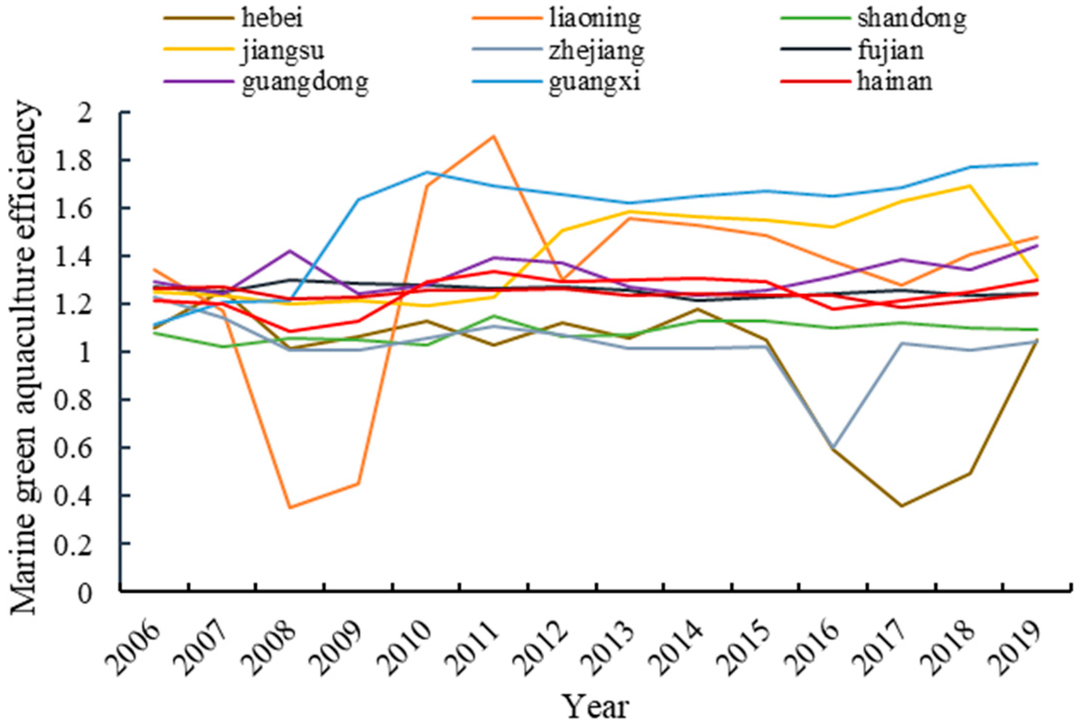
3.1.1. Efficiency Measurement and Spatial–Temporal Characteristics Analysis of Marine Green Aquaculture in China

The Super-SBM model was used to measure the efficiency of marine green aquaculture in China from 2006 to 2019, and the specific results are shown in Figure 1, which shows the changes in seawater green aquaculture efficiency in each province from 2006 to 2019.

From 2006 to 2019, the efficiency of marine green aquaculture in nine coastal provinces in China fluctuated between 0.35 and 1.91. From the overall average point of view, the efficiency of marine green aquaculture in China showed a fluctuating upward trend of first decreasing, then rising, and then decreasing again, with a fluctuation range of (1.08, 1.34), which still has large room for improvement. In 2016, except in Hebei and Liaoning, the efficiency value of marine green aquaculture in other provinces was above 1, and in 2019, the efficiency value of marine green aquaculture in all provinces was above 1. Therefore, there are great differences in the efficiency of marine green aquaculture in time and space.

There are obvious differences in the efficiency of marine green aquaculture among different regions. Among the three major marine economic circles, the average efficiency of marine green aquaculture in the southern marine economic circle is the highest, followed by the eastern marine economic circle and the northern marine economic circle. In terms of the northern marine economic circle, the average marine green aquaculture efficiency in Hebei is the lowest and lower than 1, and the average efficiency in Liaoning is the highest, followed by Shandong. In terms of the eastern marine economic circle, the average efficiency from large to small is Jiangsu and then Zhejiang. In terms of the southern marine economic circle, the average efficiency from large to small is as follows: Guangxi, Guangdong, Fujian, and Hainan.

The efficiency of marine green aquaculture in coastal provinces showed obvious differences in time series. In the northern marine economic circle, the efficiency of the Liaoning and Hebei provinces fluctuated greatly. Among them, the efficiency of marine green aquaculture in Liaoning showed a fluctuating upward trend after first decreasing, then decreasing, and then rising, reaching the lowest value of all observed samples in 2008 and the highest value of all observed samples in 2011. The overall efficiency of marine green aquaculture in Shandong province did not fluctuate much and showed a slight upward trend during the observation period. In the eastern marine economic circle, the efficiency of marine green aquaculture in Jiangsu showed a fluctuating upward trend, while that in Zhejiang showed a fluctuating downward trend. In the southern marine economic circle, the marine green aquaculture efficiency in Guangdong and Guangxi showed a fluctuating upward trend, while the marine green aquaculture efficiency in Fujian and Hainan showed a fluctuating downward trend.

In order to study the spatial disequilibrium characteristics of marine green aquaculture efficiency, Gaussian kernel density estimation was used in this research to obtain the kernel density distribution of marine green aquaculture efficiency in each coastal province, and the kernel density distribution maps for 2006, 2008, 2010, 2012, 2014, 2016, and 2019 were drawn, as shown in Figure 2.

On the whole, the pattern of the nuclear density curve changed from “convex and narrow” to “flat and wide”, indicating that the regional differences in the efficiency of marine green aquaculture in China’s coastal provinces increased. With the passage of time, the nuclear density curve shows a left-skewed distribution. When the efficiency of marine green aquaculture is high, the nuclear density is also large, indicating that the efficiency of marine green aquaculture is higher than the average value in most coastal provinces. From 2006 to 2019, the height and width of the main peak changed greatly, and the difference between the main peak and the sub-peak value is obvious, indicating that there is a certain regional difference in the efficiency of marine green aquaculture in coastal provinces. From the perspective of the number of wave peaks, except for the single-peak distribution in 2012 and 2019, the rest of the years were “double peak” or “triple peak” distributions, and there were obvious differences in high- and low-value areas, and there was two-stage or multistage differentiation. Therefore, the regional differences in the efficiency of marine green aquaculture in China were relatively significant.

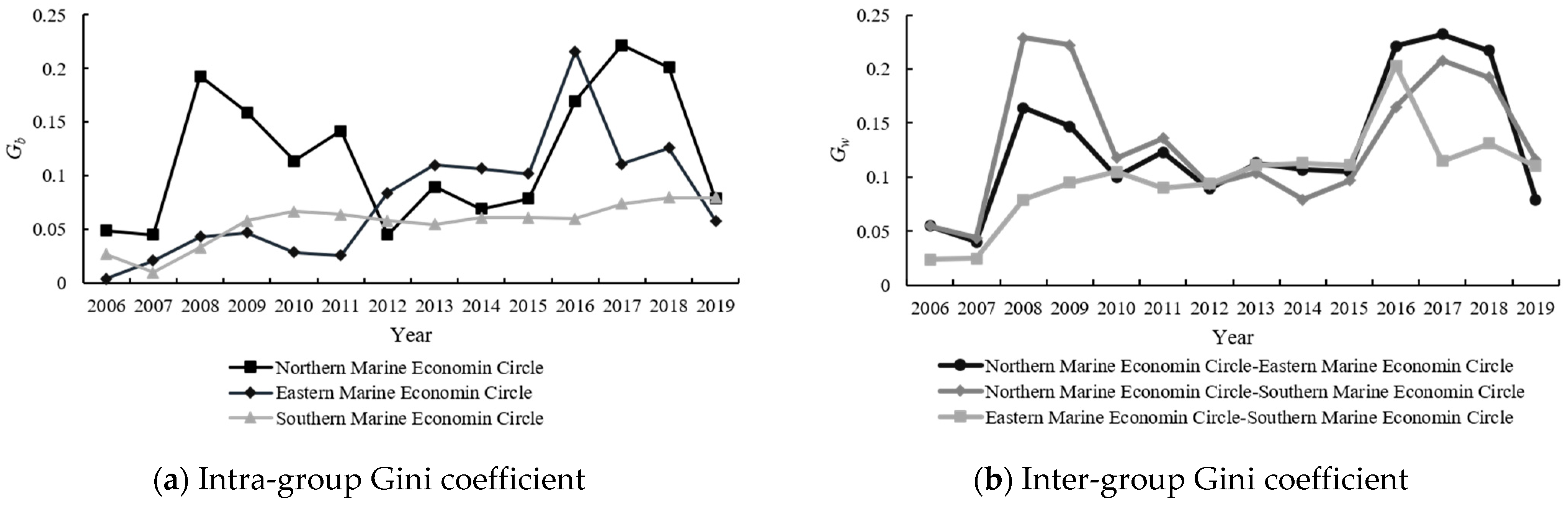
3.1.2. Extent and Decomposition of Regional Gap in the Efficiency of Marine Green Aquaculture in China

On the basis of measuring the efficiency of marine green aquaculture in coastal provinces, the regional difference in marine green aquaculture efficiency in China from 2006 to 2019 was further analyzed. The Dagum Gini coefficient was calculated and decomposed based on the three major marine economic circle groups, and the intra-group difference (G_w), inter-group difference (G_b), and supervariable density (G_t) were obtained, and the contribution rate of each part to the overall difference was further obtained, as shown in

Table 3. Dagum Gini coefficient and decomposition of green aquaculture efficiency in seawater.

Year	Total G	Within a Group		Between Groups		Hypervariable Density
		Gw	Rate of Contribution (%)	Gb	Rate of Contribution (%)	Gt	Rate of Contribution (%)
2006	0.040	0.011	0.274	0.011	0.288	0.017	0.437
2007	0.032	0.008	0.250	0.018	0.568	0.006	0.182
2008	0.130	0.026	0.199	0.102	0.790	0.001	0.011
2009	0.133	0.029	0.221	0.101	0.763	0.002	0.016
2010	0.098	0.028	0.286	0.041	0.421	0.029	0.293
2011	0.106	0.030	0.286	0.032	0.304	0.044	0.410
2012	0.080	0.021	0.261	0.041	0.507	0.019	0.232
2013	0.096	0.026	0.273	0.021	0.217	0.049	0.509
2014	0.086	0.025	0.290	0.010	0.121	0.051	0.589
2015	0.092	0.026	0.283	0.023	0.252	0.043	0.465
2016	0.159	0.040	0.249	0.070	0.440	0.049	0.311
2017	0.156	0.041	0.263	0.085	0.542	0.030	0.194
2018	0.155	0.042	0.271	0.070	0.452	0.043	0.276
2019	0.096	0.028	0.294	0.046	0.481	0.021	0.225

.

It can be seen from Table 3 that the overall Gini coefficient value of China’s marine green aquaculture efficiency shows a fluctuating upward trend, with the lowest Gini coefficient value of 0.032 in 2007 and the maximum value of 0.159 in 2016. The rise in the overall Gini coefficient means that in the process of the overall improvement in the efficiency of mariculture in China, the gap between the efficient provinces and the inefficient provinces is widening, and it is necessary to coordinate the pace of development among different regions to accelerate the green transformation of mariculture fishery. The overall Gini coefficient of China’s seawater green aquaculture efficiency experienced two rapid increases from 2006 to 2019, the first time from 0.032 in 2007 to 0.130 in 2008 and the second time from 0.092 in 2015 to 0.159 in 2016. Further, due to the impact of the global financial crisis in 2008, the fishery cost continues to rise, the consumption demand for aquatic products is relatively low, and the development of marine aquaculture fishery is full of uncertainties, which further leads to the difference in the change in domestic green marine aquaculture efficiency and aggravates the regional difference in the efficiency of green marine aquaculture [47].

After two years of a high differentiation degree, the regional difference degree of marine green aquaculture efficiency in 2010 was alleviated due to the improvement in global investment and trade, economic recovery, and domestic policy support. Affected by the South China Sea arbitration case in 2016, China is facing more and more prominent geopolitical risks. As time goes by [48], after the Sino-US trade war broke out in 2018, China’s aquaculture industry is facing increasing challenges and competitive pressure, which further stimulates the differentiation in China’s seawater green aquaculture efficiency [49]. Further, whether it was the global financial crisis in 2008, the South China Sea arbitration case in 2016, or the Sino-US trade war in 2018, the southern marine economic circle alleviated the impact brought by a series of external events by virtue of its excellent risk resistance ability and the strong resilience of marine fishery [50,51]. The efficiency of green seawater cultivation in the southern marine economic circle is more stable than that in the eastern and northern marine economic circles, while the efficiency of green seawater cultivation in the eastern and northern marine economic circles fluctuates greatly, especially in the northern marine economic circle. Figure 1 shows that when facing external shocks, the efficiency of green seawater cultivation in Liaoning and Hebei in the northern marine economic circle often shows large fluctuations. It shows a rapid decline, which has brought serious differences to the efficiency of marine green aquaculture in China. Until 2019, ten ministries and commissions jointly issued Several Opinions on Accelerating the Green Development of Aquaculture Industry, which proposed to accelerate the construction of the spatial pattern, industrial structure, and production mode of green development in the aquaculture industry and also emphasized the importance of coordination and cooperation, which provided policy guidance for coastal provinces to explore the green transformation of marine aquaculture fishery according to local conditions. Thus, the regional differences in the efficiency of marine green aquaculture in China can be alleviated.

From the point of view of the difference within the group, it shows the evolution law of first rising and then falling and then rising and then falling. The intra-regional development gap was 0.011 in 2006 and reached 0.028 in 2019, with a cumulative increase of 154.545%, reaching the lowest value of 0.008 in 2007 and the highest value of 0.042 in 2018. From the perspective of contribution rate, the contribution rate of intra-regional differences in the observation period is second in 9 years and third in the remaining 5 years. In summary, the average contribution rate of intra-regional differences is 0.264, which is the third source of regional differences. As can be seen from Figure 3, from the change trend, the intra-group Gini coefficients of the three major marine economic circles have significantly increased from 2006 to 2019, which indicates that the regional gap in the efficiency of marine green aquaculture in China is constantly expanding. From the perspective of the fluctuation amplitude, the fluctuation amplitude of the southern marine economic circle is smaller, and the intra-group Gini coefficient of most years is smaller than that of the northern and eastern marine economic circles. Therefore, on the whole, the intra-regional gap of the southern marine economic circle is small. From the perspective of the intra-group average Gini coefficient, the intra-group average Gini coefficient of the northern marine economic circle is 0.118, that of the eastern marine economic circle is 0.077, and that of the southern marine economic circle is 0.056. Therefore, among the three major marine economic circles, the intra-regional gap is the largest in the northern marine economic circle, followed by the eastern marine economic circle. The southern maritime economic circle has the smallest intra-regional gap.

From the point of view of the difference between groups, it shows the evolution law of fluctuation rising. The intra-regional development gap was 0.011 in 2006 and reached 0.046 in 2019, with a cumulative increase of 318.182%, reaching the highest value of 0.102 in 2008 and the lowest value of 0.010 in 2014. From the perspective of contribution rate, the contribution rate of inter-regional differences in the observation period is the first in 9 years, the second in 2 years, and the third in 3 years. In summary, the average contribution rate of inter-regional differences is 0.439, which belongs to the first source of regional differences. As can be seen from Figure 3, during 2006-2019, the inter-group Gini coefficients of north–east, north–south, and east–south have significantly increased, in which the north–east marine economic circle and the north–south marine economic circle have experienced a fluctuating upward trend of first decreasing and then increasing, then decreasing again. On the other hand, the east–south marine economic circle showed an evolutionary law of first rising and then falling and then rising and falling again. The mean inter-group Gini coefficients of the north–east, north–south, and east–south were 0.128, 0.133, and 0.100, respectively. Compared with the north–east and north–south marine economic circles, the inter-group Gini coefficients of the east–south marine economic circle fluctuated less, and the inter-group Gini coefficients of the east–south marine economic circle were smaller than those of the other two combinations in most years. Therefore, the regional differences between the northern–eastern marine economic circle and the northern–southern marine economic circle are more obvious.

In terms of supervariable density, it shows the evolution law of fluctuation rise. The intra-regional development gap was 0.017 in 2006 and reached 0.021 in 2019, with a cumulative increase of 23.529%, reaching the lowest value of 0.001 in 2008 and the highest value of 0.051 in 2014. From the perspective of contribution rate, the contribution rate of supervariable density in the observation period is the first in 5 years, the second in 6 years, and the third in 3 years. In summary, the average contribution rate of intra-regional differences is 0.296, which belongs to the second source of regional differences. During the whole observation period, the contribution rate of supervariable density is relatively large, indicating that the impact of cross-overlap between different regions on the overall difference is an important reason for the overall gap in the efficiency of marine green aquaculture.

To sum up, the main source of the regional gap in the efficiency of marine green aquaculture in China is the disequilibrium of the efficiency of marine green aquaculture between regions, and the relative contribution of intra-regional differences is small. This is consistent with the actual situation of the three major marine economic circles. In the future, determining how to coordinate the regional gap between the three major marine economic circles in marine green aquaculture is the main direction to reduce the regional gap in the efficiency of marine green aquaculture.

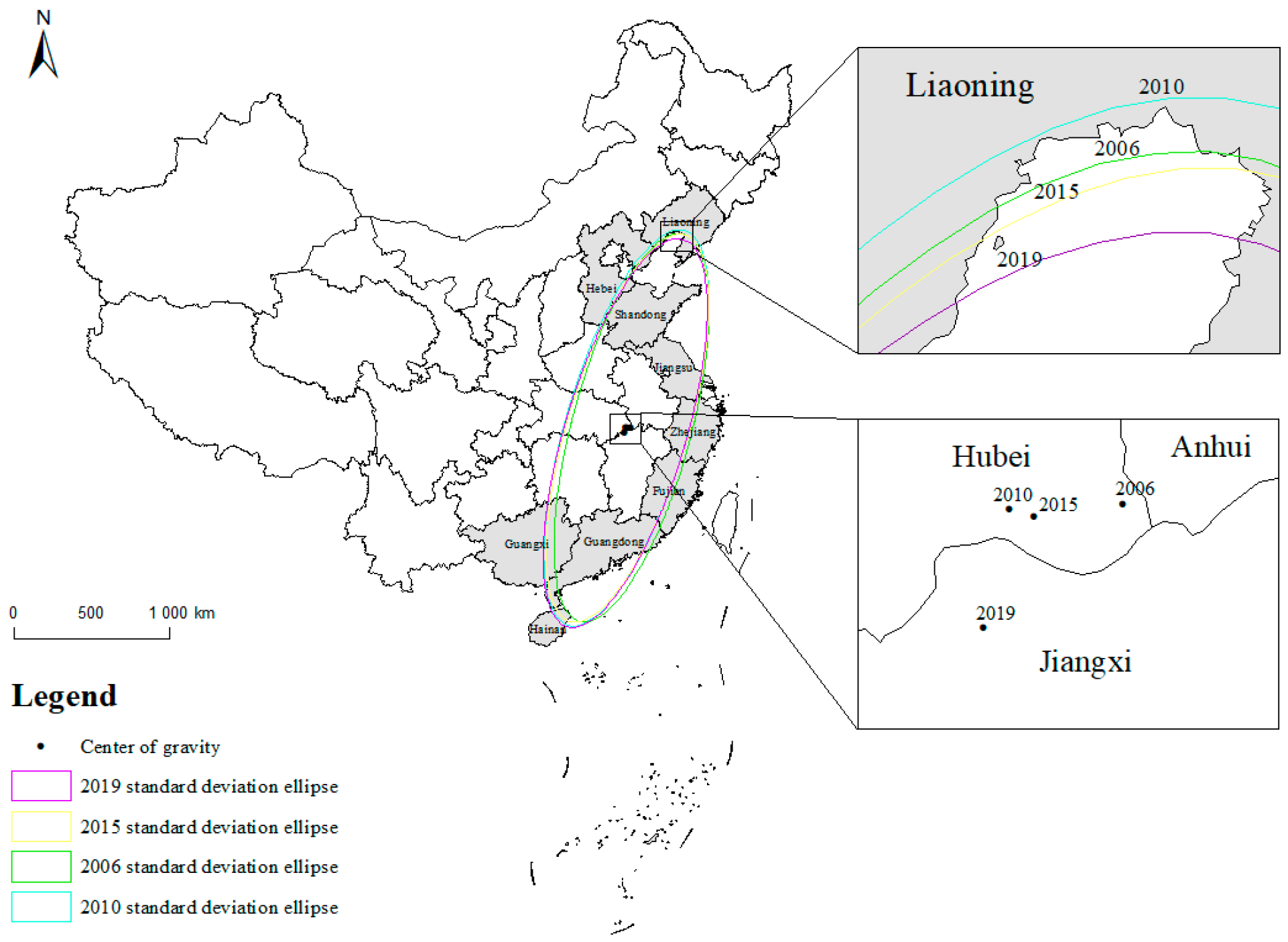
3.1.3. Spatial Distribution Pattern of Marine Green Aquaculture Efficiency in China

This research measured the center of gravity and standard deviation ellipse of marine green aquaculture efficiency in our country by using the ArcGIS10.8 software. By analyzing the center of gravity of marine green aquaculture efficiency and its changing trajectory, the changing direction of efficiency space can be determined. By analyzing the direction of the major semi-axis of the standard deviation ellipse, we can understand the main distribution direction of the marine green aquaculture efficiency, and by analyzing the direction of the short semi-axis of the standard deviation ellipse, we can understand the main distribution range of the marine green aquaculture efficiency. By analyzing the change in rotation angle, we can understand the change in the main direction of marine green aquaculture efficiency. By analyzing the area of the standard deviation ellipse and its change, the development trend of marine green aquaculture efficiency can be judged. The relevant parameters of the spatial distribution center of gravity and standard deviation ellipse of marine green aquaculture efficiency are shown in

Table 4. Barycenter standard deviation ellipse parameter table of green aquaculture efficiency in seawater.

Year	Barycentric Coordinates	Direction	Distance Traveled/km	Angle of Turn θ/°	Major Half Axis/km	Short Half Axis/km	Area of Ellipse/10 Thousand km2
2006	(116.06° E, 29.89° N)			15.020	1289.036	383.353	155.208
2010	(115.72° E, 29.92° N)	West by north	37.880	16.430	1323.330	391.208	162.602
2015	(115.79° E, 29.89° N)	East by south	8.560	16.640	1294.946	385.547	156.812
2019	(115.60° E, 29.62° N)	South by west	36.860	16.730	1299.942	388.466	158.610

, and the evolution diagram of the spatial pattern of marine green aquaculture efficiency in China in 2006, 2010, 2015, and 2019 was drawn, as shown in Figure 4.

In terms of the distribution and change in the center of gravity, it can be seen from Figure 4 that the center of gravity of China’s marine green aquaculture efficiency is not in the nine coastal provinces, which is caused by the geographical shape of the nine coastal provinces. The center of gravity of the observation year is roughly in the middle of China’s coastal provinces, indicating that the difference in China’s marine green aquaculture efficiency in the north–south direction is not obvious. As can be seen from Table 4, the movement track of the barycenter coordinates shows that in 2010, the barycenter moved 37.880 km from west to north, with little change in the north–south direction, indicating that the efficiency of marine green aquaculture in the western coastal provinces of China (such as Guangxi and Hebei) has improved greatly. In 2015, the center of gravity moved 8.560 km to the east–south direction, which indicates that the efficiency of marine green aquaculture in the southeast of China’s coastal provinces (such as Guangdong and Fujian) has improved greatly. In 2019, the center of gravity moved 36.860 km to the east–south direction, which indicates that the efficiency of marine green aquaculture in the southwest of China’s coastal provinces (such as Guangxi) has improved greatly. On the whole, the center of gravity shifted to the south from 2006 to 2019, indicating that the efficiency of marine green aquaculture in southern China’s marine economic circle has improved.

From the perspective of the standard deviation ellipse, the standard deviation ellipse of marine green aquaculture efficiency in China from 2006 to 2019 was mainly located in the eastern coastal area of China. On the whole, the standard deviation ellipse moved eastward, and the area of the ellipse showed an overall trend of increasing, indicating that the coverage area of the standard deviation ellipse was further expanded. Angle θ increased year by year, from 15.020° in 2006 to 16.730° in 2019, indicating that the spatial pattern of marine green aquaculture efficiency in China was deflected by 1.710° from northeastern–southwest to due east–west. Therefore, on the whole, the spatial pattern of marine green aquaculture efficiency in China presents a northeastern–southwest pattern, and the trend is gradually shifting in a clockwise direction. According to the change in the major axis, the length of the major axis showed an increasing trend from 2006 to 2019, increasing from 1289.036 km in 2006 to 1299.942 km in 2019, indicating that the spatial pattern of marine green aquaculture efficiency in the northeastern–southwest direction has a diffusion trend along the main axis direction. According to the changes of the short semi-axis, the length of the short semi-axis showed an increasing trend from 2006 to 2019, increasing from 383.353 km in 2006 to 388.466 km in 2019, indicating that the spatial pattern of marine green aquaculture efficiency in the northeastern–southwest direction has a diffusion trend in the auxiliary axis direction. On the whole, the spatial distribution of marine green aquaculture efficiency in China has experienced a trend of first diffusion, then agglomeration, and then diffusion in the direction of long and short axes.

From the perspective of the three major marine economic circles, the center of gravity and standard deviation ellipse of China’s marine green aquaculture efficiency are mainly distributed in the eastern and southern marine economic circles of China’s coastal areas and tend to shift to the southern marine economic circle as time goes by. This is because the coastal provinces on which the eastern and southern marine economic circles rely have a higher level of economic development, have sufficient funds, have advanced green aquaculture technology, and are more attractive to mariculture professionals.

The focus of China’s marine green aquaculture efficiency has shown a trend of westward movement after 2010, which is due to “the promulgation of the 11th Five-Year Plan for National Fishery Development” and “the Outline of the National 11th Five-Year Plan for Marine Science and Technology Development”. Hebei Province has adopted artificial reefs, increased aquaculture, and three-dimensional aquaculture in shallow seas. Effectively restoring marine fishery resources and the ecological environment and promoting the development of ecological industries, by creating an advantageous aquaculture belt, Guangxi develops green and healthy aquaculture and promotes the improvement in marine green aquaculture efficiency to a certain extent. After 2015, it has shown a southward trend, which is because the southern marine economic circle has always had a high level of external development. After “the promulgation of the 12th Five-Year Plan for National Fishery Development”, the focus of fishery development in the coastal provinces of the southern marine economic circle has continuously shifted to an ecologically healthy aquaculture industry and environmentally friendly breeding fishery, and the efficiency of marine green aquaculture has been improved. This has driven the center of gravity south. In 2019, the center of gravity moved south because, after ten ministries and commissions jointly issued the “Several Opinions on Accelerating the Green Development of Aquaculture Industry”, the southern marine economic circle continued to strengthen the treatment of aquaculture wastewater and waste, attach importance to the ecological restoration function of aquaculture, and actively develop ecological and healthy aquaculture fisheries, which greatly promoted the improvement in the efficiency of marine green aquaculture.

3.2. Dynamic Evolution of Marine Green Aquaculture Efficiency in China

3.2.1. Static Analysis Results of Spatial Markov Chain

In this research, it is assumed that the efficiency of marine green aquaculture follows the first-order Markov distribution and has a stable transfer probability, and the spatial Markov transfer probability matrix is obtained using the quartile method. According to the intervals of 0~1/4, 1/4~1/2, 1/2~3/4, and 3/4~1, the efficiency state is divided into four categories: low level, lower level, higher level, and high level. If the efficiency of marine green aquaculture in the next year still belongs to the same efficiency type as the previous year, then the transfer of this area is defined as self-locking. If the efficiency of marine green aquaculture in the next year increases compared with the previous year, the regional transfer is defined as the upward transfer type, and the reverse is the downward transfer type. As can be seen from

Table 5. Spatial Markov transition probability matrix of green aquaculture efficiency in seawater.

Spatial Lag	t/t + 1	Frequency	Low Level	Lower Level	Higher Level	High Level
No lag	Low level	211	0.919	0.081	0	0
	Lower level	210	0.005	0.862	0.133	0
	Higher level	206	0	0.010	0.879	0.112
	High level	193	0	0	0.016	0.985
1	Low level	36	0.917	0.083	0	0
	Lower level	29	0	0.966	0.035	0
	Higher level	5	0	0	0.800	0.200
	High level	1	0	0	0	1
2	Low level	136	0.934	0.066	0	0
	Lower level	109	0	0.881	0.119	0
	Higher level	88	0	0	0.932	0.068
	High level	26	0	0	0.077	0.923
3	Low level	34	0.853	0.147	0	0
	Lower level	67	0.015	0.821	0.164	0
	Higher level	78	0	0.013	0.859	0.128
	High level	58	0	0	0.017	0.983
4	Low level	5	1.000	0	0	0
	Lower level	5	0	0.400	0.600	0
	Higher level	35	0	0.029	0.800	0.171
	High level	108	0	0	0	1.000

Note: 1, 2, 3, and 4 in the table represent low, lower, higher, and high levels of spatial lag, respectively. Frequency represents the summary of the number of provinces.

, in the traditional Markov transition probability matrix, the self-locking probability of provinces with the high-level state is the highest, which is 98.5%. The self-locking probability of provinces with the lower-level state is the lowest (86.2%), and the state migration mainly occurs in the type of “lower level → higher level”. The high-level provinces have the highest locking probability, and the low-level provinces have a small probability of state transfer, which indicates that advantages and disadvantages coexist in the process of marine green aquaculture efficiency from unbalanced to balanced, and breaking the development bottleneck of low-level provinces is the key to achieving balanced development.

As can be seen from Table 5, when considering the type of spatial lag in the neighborhood, the self-locking probabilities of provinces with a low-level status are 91.7%, 96.6%, 80.0%, and 100%, respectively, and those of provinces with lower-level status are 93.4%, 88.1%, 93.2%, and 92.3%, respectively. The self-locking probabilities of the provinces with a higher-level status were 85.3%, 82.1%, 85.9%, and 98.3%, and the self-locking probabilities of the provinces with a high-level status were 100%, 40%, 80%, and 100%, respectively. Therefore, the following conclusions were made:

① There are four convergence club characteristics of marine green aquaculture efficiency: low level, lower level, higher level, and high level. When the spatial lag is considered, on the one hand, most of the probability values on the diagonal are higher than those on the non-diagonal, indicating that the efficiency of marine green aquaculture in each coastal province is stable, the internal fluidity is strong, and the probability of maintaining the initial state is large. On the other hand, low-level and lower-level provinces are more susceptible to the influence of neighboring provinces, and the higher the level of neighboring provinces, the greater the probability of provincial transfer.

② Spatial proximity plays a key role in the state transfer of marine green aquaculture efficiency. The higher the efficiency of marine green aquaculture in neighboring provinces, the greater the effect on improving the efficiency of marine green aquaculture in the province. When considering the type of neighborhood lag, the probability of low-level to lower-level transfer is 8.3%, 6.6%, 14.7%, and 40%. The probability of the lower level moving to the higher level was 3.5%, 11.9%, 16.4%, and 60%. Therefore, provinces with a high spatial lag and high level have the most significant effect on the improvement in the efficiency of marine green aquaculture in their own province, that is, the higher the efficiency of marine green aquaculture in neighboring provinces, the more beneficial it is to promote the improvement in marine green aquaculture efficiency. However, it is worth noting that for provinces with low efficiency of marine green aquaculture, if the gap between neighboring provinces and their efficiency is too large, the positive spillover effect may be reduced.

③ The state transfer of marine green aquaculture efficiency usually occurs between similar horizontal states, and there is less “leapfrog” transfer. The non-diagonal figures are evenly distributed on both sides of the diagonal line, indicating that there is both an upward trend and a downward possibility of marine green aquaculture efficiency transfer. Overall, the probability of moving down is lower than moving up.

In summary, the state transfer trend of marine green aquaculture efficiency has a certain “path dependence” effect, and it is difficult to achieve leapfrog development. To give full play to the spillover effect of neighboring areas, regions with high and higher levels of green seawater aquaculture efficiency should drive the improvement in green seawater aquaculture efficiency of neighboring areas with low and lower levels through channels such as policy spread, technology spillover, and factor flow, and break the self-lock of regions with low and lower levels of green seawater aquaculture efficiency through assistance and cooperation, promoting the coordinated development of green seawater aquaculture in all regions.

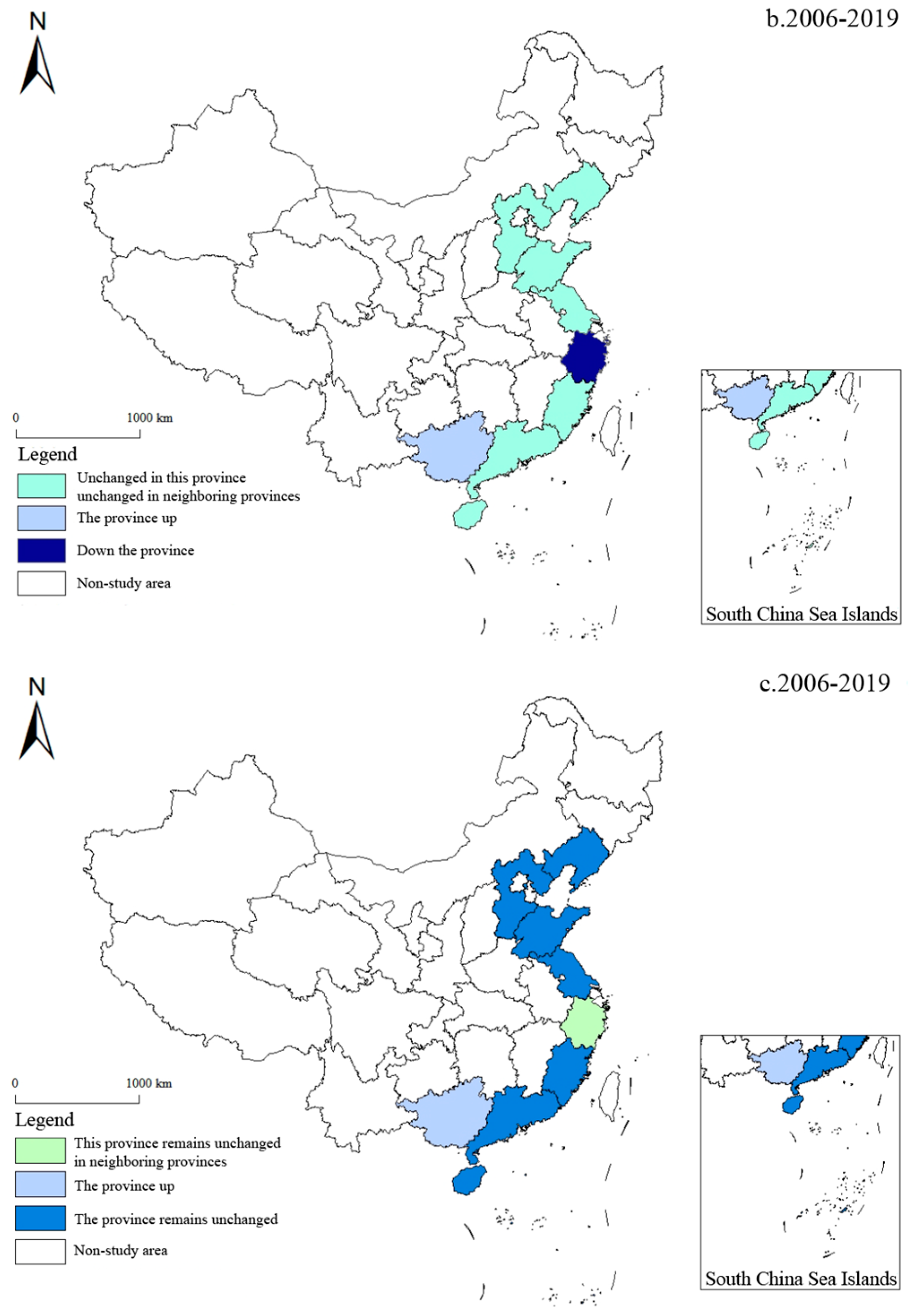
3.2.2. Dynamic Analysis Results of Spatial Markov Chain

The ArcGIS10.8 (Environmental Systems Research Institute, Redlands, CA, USA) software was further used to visualize the transfer of marine green aquaculture efficiency and analyze the dynamic evolution characteristics of marine green aquaculture efficiency in China. See Figure 5 for details.

From Figure 5, it can be seen that from 2006 to 2019, there is one province with its own province rising and its neighboring provinces unchanged (Guangxi), one province with its own province falling and its neighboring provinces unchanged (Zhejiang), and seven provinces with their own province rising and their neighboring provinces unchanged (Liaoning, Hebei, Shandong, Jiangsu, Fujian, Guangdong, and Hainan). There is no such thing as one province going up and one neighboring province going up and one province going down and one neighboring province going down. To sum up, the correlation effect of marine green aquaculture efficiency in China is generally good, and most provinces are in a constant or upward transfer state; only Zhejiang Province has a backward trend of downward transfer. The possible reasons are that the proportion of fish farming in the economy of Zhejiang Province is still large [52], and the growth mode of extensive fisheries is still dominant, which leads to the downward transfer of the efficiency of marine green aquaculture in Zhejiang Province.

3.3. Analysis of Driving Factors of Regional Gap in Marine Green Aquaculture Efficiency in China

The factor detection results show that, overall, the explanatory strength of each driving factor for the regional gap in the efficiency of marine green aquaculture in China, from the largest to the smallest, is the number of professional practitioners of marine aquaculture (x1), the number of aquatic technology extension institutions (x2), the output of marine aquaculture (x8), the area of marine aquaculture (x4), the capacity of carbon sequestration (x10), and the number of marine aquaculture motor fishing vessels (production vessels) at the end of the year (x3), the number of fishermen in technical training (x9), per capita disposable income of fishermen (x7), output value of mariculture (x6), and the number of seawater seedlings (x5). Among them, the number of marine aquaculture professionals (x1) is the core driver and plays a leading role in the regional gap in the efficiency of marine green aquaculture in China. Based on the detection and analysis results of geographical detector factors, the q value variation in driving factors for the regional gap in the efficiency of marine green aquaculture in China was plotted, as shown in Figure 6.

As can be seen from Figure 6, during 2006–2019, the q values of the number of professional mariculture practitioners (x1), the number of aquatic technology extension institutions (x2), the number of seawater seedlings (x5), and the output value of mariculture (x6) showed an increasing trend, and the increasing degree was in the following order from large to small: x2 (67.387%), x1 (60.310%), x6 (29.820%), and x5 (29.323%). The q values of other driving factors showed a decreasing trend, and the decreasing degree was as follows: x7 (−39.035%), x8 (−21.523%), x10 (−10.415%), x4 (−8.963%), x3 (−4.628%), and x9 (−0.304%). This indicates that the explanatory power of the number of mariculture professionals (x1), the number of aquatic technology extension institutions (x2), the number of seawater seedlings (x5), and the output value of mariculture (x6) is increasing. At the end of the year, the explanatory power of mariculture motor fishing vessels (production fishing vessels) (x3), mariculture area (x4), per capita disposable income of fishermen (x7), mariculture output (x8), technical training number of fishermen (x9), and carbon sequestration capacity (x10) continued to decline.

The reason for this is that with the continuous progress of the green transformation of mariculture, more and more attention is paid to the investment in human capital, technology, and improved seed cultivation. The number of professional practitioners in mariculture better reflects the inflow of professional talents, and the number of aquatic technology extension institutions reflects the technical investment in mariculture to a certain extent. The number of seawater seedlings reflects the input of seedlings to a certain extent. Economically developed coastal areas are more attractive to professionals and have a higher level of technical input, and more resources are poured into seedling cultivation and investment, which has a strong siphon effect on human capital elements. The number of professional mariculture practitioners (x1), the number of aquatic technology extension institutions (x2), and the number of seawater seedlings (x5) showed an increasing explanatory power to the regional gap in the efficiency of mariculture. To promote the green transformation of mariculture under the guidance of the “two mountains theory”, it is necessary to focus on the win–win situation of economic and ecological environmental benefits. The output value of mariculture (x6), as an important economic index of the efficiency of mariculture, has a high spatial matching degree with the efficiency of mariculture.

The results of interaction detection show that the interaction of factors in each year is double-factor strengthening or nonlinear strengthening. The interaction of factors with an interaction q ≥ 0.9 is shown in

Table 6. Each driver interacts with the factor type.

Year	Factor of Interaction
2006	x1∩x3; x1∩x10; x2∩x3; x3∩x8; x7∩x8*
2008	x1∩x3; x1∩x4; x1∩x7*; x1∩x8; x1∩x9; x1∩x10; x2∩x3; x2∩x4; x2∩x7; x2∩x8*; x2∩x9; x2∩x10; x3∩x7*; x3∩x8*; x4∩x8*; x5∩x8*; x6∩x8*; x7∩x8*; x7∩x9*; x8∩x9*; x8∩x10*; x9∩x10
2010	x1∩x9; x2∩x9; x4∩x9*
2012	x1∩x4; x1∩x10*; x2∩x4
2014	x1∩x7; x1∩x9; x2∩x9
2016	x1∩x2; x2∩x10; x3∩x6; x3∩x9
2019	x1∩x8*; x2∩x3*; x2∩x6*; x2∩x8*; x5∩x8; x6∩x7; x7∩x8

Note: This table only lists the interaction factors for q(xi∩xj) ≥ 0.9. Among them, the upper right marked with * indicates that the interaction of this group of factors is a double-factor strengthening, that is, q(xi∩xj) > Max[q(xi), q(xj)]; unlabeled * indicates nonlinear strengthening, that is, q(xi∩xj) > q(xi) + q(xj).

.

As can be seen from Table 6, the explanatory power of the interaction of the two factors on the regional gap in the efficiency of marine green aquaculture is more than 90%, which is much higher than the explanatory power of a single factor. It can be seen that the regional gap in the efficiency of marine green aquaculture is the result of multiple driving factors. Among them, there are x1 and x2 factors in the factor groups with an interaction q ≥ 0.9 in each year, which further verifies that the number of professional mariculture practitioners (x1) is the core driving factor of the regional gap in the efficiency of mariculture. The explanatory power of the number of mariculture professionals (x1), the number of aquaculture technology extension institutions (x2), and the number of mariculture motor fishing vessels (production fishing vessels) at the end of the year (x3) after interacting with other driving factors was significantly greater than the sum of the two factors, which was characterized as nonlinear enhancement. This shows that the number of marine aquaculture professionals (x1), the number of aquatic technology extension institutions (x2), and the number of marine aquaculture motor fishing vessels (production fishing vessels) at the end of the year (x3), when combined with other driving factors, will have a strong driving effect on the efficiency of marine green aquaculture.

4. Conclusions and Suggestions

4.1. Conclusions

The main research conclusions are as follows: (1) From 2006 to 2019, the efficiency of marine green aquaculture in China showed a fluctuating upward trend and had large room for improvement, and the efficiency of marine green aquaculture showed obvious differences in time series. The nuclear density curve of China’s marine green aquaculture efficiency changes from “convex and narrow” to “flat and wide”, indicating that the regional difference in China’s marine green aquaculture efficiency is enlarged, and there is a two-stage or multi-level differentiation phenomenon. On the whole, from 2006 to 2019, the overall Gini coefficient value of marine green aquaculture efficiency showed a fluctuating upward trend, which indicates that the regional gap of marine green aquaculture efficiency in China continues to expand. From the decomposition situation, the Gini coefficients of the three major marine economic circles have significantly increased, and the main source of the regional gap in the efficiency of marine green aquaculture in China is the disequilibrium of the efficiency of marine green aquaculture in the inter-region. Compared with the northern and eastern marine economic circles, the gap in the southern marine economic circle is the smallest. In terms of the change in the center of gravity, the center of gravity of China’s marine green aquaculture efficiency showed a southward shift pattern, and the marine green aquaculture efficiency in southern China’s marine economic circle was improved. In terms of the variation in the standard deviation ellipse, the efficiency of marine green aquaculture in China presents a spatial distribution pattern from northeast to southwest. In terms of the length of the major half axis and short half axes, the spatial distribution of the efficiency of marine green aquaculture in China has experienced the evolution trend of first diffusion, then agglomeration, and then diffusion. The center of gravity and standard deviation ellipse of China’s marine green aquaculture efficiency are mainly distributed in the eastern and southern marine economic circles of China’s coastal areas and tend to shift to the southern marine economic circles as time goes by.

(2) When spatial lag is considered, most of the probability values on the diagonal are higher than those on the non-diagonal, indicating that the efficiency of marine green aquaculture in each coastal province is stable and the probability of maintaining the initial state is high. There is both an upward trend and a possibility of downward transfer in marine green aquaculture efficiency, and the probability of downward transfer is lower than that of upward transfer. Spatial proximity plays a key role in the state transfer of marine green aquaculture efficiency. The higher the efficiency of marine green aquaculture in neighboring provinces, the more conducive it is to promoting the improvement in marine green aquaculture efficiency, but the transfer trend of marine green aquaculture efficiency has a certain “path dependence” effect, and it is difficult to achieve leapfrog development.

(3) During 2006-2019, the q values of the number of professional mariculture practitioners, the number of aquatic technology extension institutions, the number of seawater seedlings, and the output value of mariculture showed an upward trend, while the q values of other driving factors showed a downward trend, among which the number of professional mariculture practitioners was the core driving factor. It plays a leading role in the regional gap in the efficiency of marine green aquaculture in China. The explanatory power of the interaction of the two factors on the regional gap in marine green aquaculture efficiency is more than 90%, which is much higher than the explanatory power of a single factor. The regional gap in marine green aquaculture efficiency is the result of multiple driving factors. When the number of professional mariculture practitioners, the number of aquaculture technology extension institutions, and the number of mariculture motor fishing vessels (production fishing vessels) at the end of the year are combined with other driving factors, they will have a strong driving effect on the efficiency of marine green aquaculture.

4.2. Suggestions

To sum up, the imbalance and insufficiency of China’s mariculture green transformation will inevitably become a constraint to promoting the high-quality development of fisheries. Only by coordinating the green transformation of mariculture and continuously reducing the regional gap in the efficiency of mariculture can we continue to promote the green development of China’s marine aquaculture fisheries. Therefore, the following suggestions are put forward in this research: (1) While promoting areas with high marine green aquaculture efficiency to a new level of green development, we must tap into the green transformation potential of areas with low marine green aquaculture efficiency. On the one hand, resources should be tilted to areas with low marine green aquaculture efficiency, more policy support should be given to areas with low marine green aquaculture efficiency, and technical assistance and talent input from areas with high marine green aquaculture efficiency should be promoted to areas with low marine green aquaculture efficiency. On the other hand, we must accelerate the research and development and application of marine green aquaculture technology in inefficient areas, reduce carbon emissions, nitrogen and phosphorus pollutants, and other undesired outputs from the root, improve the carbon sequestration of marine aquaculture fisheries, and achieve the steady growth of economic output, the ecological environment, and green development. In view of the regional gap in the efficiency of marine green aquaculture in China, it is necessary to give play to the demonstration and leading role of areas with high efficiency of marine green aquaculture, form a model of green transformation, and learn and promote successful experiences in areas with a low efficiency of marine green aquaculture. In view of the regional gap in the efficiency of marine green aquaculture in China, it is necessary to explore the local model of green transformation of marine aquaculture based on the successful experience of demonstration areas and formulate a green development policy of marine aquaculture with local characteristics. We should build a sharing platform for marine green aquaculture talents and technical information within the three major marine economic circles, enhance cooperation and exchanges among the economic circles, and promote the green transformation of marine aquaculture in coordination among the economic circles. In the context of the northeast to southwest spatial distribution pattern of marine green aquaculture efficiency in China, the center of marine green aquaculture efficiency has been shifting to the southern marine economic circle, and the marine aquaculture fishery in the southern marine economic circle should continue to maintain a good momentum of development and promote the marine aquaculture fishery to become more efficient, intelligent, and green.

(2) On the premise of considering the spatial lag, it is necessary to fully grasp the heterogeneity of resource endowments in provinces with different levels of status, promote the upward transfer of marine green aquaculture efficiency in provinces with low and lower levels of status, continue to promote the green transformation of marine aquaculture in provinces with high and higher levels of status, and guard against the downward transfer of their level status. On the one hand, by promoting the optimization of mariculture structure, the research and development of advanced mariculture technology, the breeding of improved varieties, and their scientific combination, the downward transfer trend of the efficiency of mariculture was reversed. On the other hand, the provinces with a high-level and higher-level state produce a technology spillover and diffusion effect through assistance cooperation, thus driving the improvement in marine green aquaculture efficiency in neighboring provinces.

(3) By paying attention to the input and output of marine aquaculture fisheries, we can improve the quality and efficiency of the output and promote the green development of marine aquaculture fisheries. We can increase the attraction of mariculture talents, optimize the working environment of professional practitioners and improve their income level, and explore the training and education mode of new professional fishermen, so as to promote the improvement in human capital level. An incentive-compatible scientific research assessment system should be established to stimulate the enthusiasm of researchers in scientific research, so as to accelerate the research and development of advanced technology of marine green aquaculture and the transformation of results. On the basis of the rational allocation of resources, combined with technical means and talent support, we can promote the steady growth of the mariculture output value and reduce a series of pollutant emissions and carbon emissions, so as to achieve a win–win situation of economic benefits and ecological environmental benefits.

References

1. Grealis, E.; Hynes, S.; O’Donoghue, C.; Vega, A.; Van Osch, S.; Twomey, C. The Economic Impact of Aquaculture Expansion: An Input-Output Approach. Mar. Policy 2017, 81, 29–36. [Google Scholar] [CrossRef]
2. Naylor, R.L.; Hardy, R.W.; Buschmann, A.H.; Bush, S.R.; Cao, L.; Klinger, D.H.; Little, D.C.; Lubchenco, J.; Shumway, S.E.; Troell, M. A 20-Year Retrospective Review of Global Aquaculture. Nature 2021, 591, 551–563. [Google Scholar] [CrossRef] [PubMed]
3. Bjørndal, T.; Dey, M.; Tusvik, A. Economic Analysis of the Contributions of Aquaculture to Future Food Security. Aquaculture 2024, 578, 740071. [Google Scholar] [CrossRef]
4. Ton Nu Hai, A.; Speelman, S. Economic-Environmental Trade-Offs in Marine Aquaculture: The Case of Lobster Farming in Vietnam. Aquaculture 2020, 516, 734593. [Google Scholar] [CrossRef]
5. Votsi, N.E. Pathways to Protect Marine Biodiversity: Could Marine Protected Areas (MPAs) Be Benefited by Landscape Ecology? Mar. Pollut. Bull. 2023, 191, 114942. [Google Scholar] [CrossRef] [PubMed]
6. Gomes Ferreira, R.; Ferreira, J.G.; Boogert, F.-J.; Corner, R.A.; Nunes, J.P.; Grant, J.; Johansen, J.; Dewey, W.F. A Multimetric Investor Index for Aquaculture: Application to the European Union and Norway. Aquaculture 2020, 516, 734600. [Google Scholar] [CrossRef]
7. Puszkarski, J.; Śniadach, O. Instruments to Implement Sustainable Aquaculture in the European Union. Mar. Policy 2022, 144, 105215. [Google Scholar] [CrossRef]
8. Guillen, J.; Asche, F.; Carvalho, N.; Fernández Polanco, J.M.; Llorente, I.; Nielsen, R.; Nielsen, M.; Villasante, S. Aquaculture Subsidies in the European Union: Evolution, Impact and Future Potential for Growth. Mar. Policy 2019, 104, 19–28. [Google Scholar] [CrossRef]
9. Carter, C. Actor Intentions Implementing ‘Ecosystem Europe’: The Contested Case of Aquaculture. Environ. Sci. Policy 2021, 124, 305–312. [Google Scholar] [CrossRef]
10. Olin, P.G.; Smith, J.; Nabi, R. Regional Review on Status and Trends in Aquaculture Development in North America: Canada and the United States of America—2010. FAO. UC San Diego: California Sea Grant College Program. 13 January 2012. Available online: https://escholarship.org/uc/item/1946b7nm (accessed on 5 December 2023).
11. Fujita, R.; Brittingham, P.; Cao, L.; Froehlich, H.; Thompson, M.; Voorhees, T. Toward an Environmentally Responsible Offshore Aquaculture Industry in the United States: Ecological Risks, Remedies, and Knowledge Gaps. Mar. Policy 2023, 147, 105351. [Google Scholar] [CrossRef]
12. Yamane, T. Capture Fisheries and Aquaculture in Japan and the World: Current Status and Future Concern. In Marine Productivity: Perturbations and Resilience of Socio-Ecosystems; Ceccaldi, H.-J., Hénocque, Y., Koike, Y., Komatsu, T., Stora, G., Tusseau-Vuillemin, M.-H., Eds.; Springer International Publishing: Cham, Switzerland, 2015; pp. 271–281. [Google Scholar]
13. Jang, H.G.; Yamazaki, S. Community-Level Analysis of Correlated Fish Production in Fisheries and Aquaculture: The Case of Japan. Mar. Policy 2020, 122, 104240. [Google Scholar] [CrossRef]
14. Bergland, H.; Burlakov, E.; Pedersen, P.A.; Wyller, J. Aquaculture, Pollution and Fishery—Dynamics of Marine Industrial Interactions. Ecol. Complex. 2020, 43, 100853. [Google Scholar] [CrossRef]
15. Gaspar, M.B.; Carvalho, S.; Cúrdia, J.; dos Santos, M.N.; Vasconcelos, P. Restoring Coastal Ecosystems from Fisheries and Aquaculture Impacts. In Reference Module in Earth Systems and Environmental Sciences; Elsevier: Amsterdam, The Netherlands, 2023; ISBN 978-0-12-409548-9. [Google Scholar]
16. Liu, G.; Xu, Y.; Ge, W.; Yang, X.; Su, X.; Shen, B.; Ran, Q. How Can Marine Fishery Enable Low Carbon Development in China? Based on System Dynamics Simulation Analysis. Ocean Coast. Manag. 2023, 231, 106382. [Google Scholar] [CrossRef]
17. Zhang, F.; He, Y.; Xie, S.; Shi, W.; Zheng, M.; Wang, Y. Research on the Game of Fishermen’s Cooperative Behavior in Developing Marine Carbon Sink Fisheries from a Complex Network Perspective. Ocean Coast. Manag. 2023, 244, 106832. [Google Scholar] [CrossRef]
18. Nielsen, M.; Ravensbeck, L.; Nielsen, R. Green Growth in Fisheries. Mar. Policy 2014, 46, 43–52. [Google Scholar] [CrossRef]
19. Fu, X.-M.; Wu, W.-Y.; Lin, C.-Y.; Ku, H.-L.; Wang, L.-X.; Lin, X.-H.; Liu, Y. Green Innovation Ability and Spatial Spillover Effect of Marine Fishery in China. Ocean Coast. Manag. 2022, 228, 106310. [Google Scholar] [CrossRef]
20. Yan, W.; Zhong, C. The Coordination of Aquaculture Development with Environment and Resources: Based on Measurement of Provincial Eco-Efficiency in China. Int. J. Environ. Res. Public Health 2022, 19, 8010. [Google Scholar] [CrossRef]
21. Shi, X.; Xu, Y.; Dong, B.; Nishino, N. Mariculture Carbon Sequestration Efficiency in China: Its Measurement and Socio-Economic Factor Analysis. Sustain. Prod. Consum. 2023, 40, 101–121. [Google Scholar] [CrossRef]
22. Guo, W.; Dong, S.; Qian, J.; Lyu, K. Measuring the Green Total Factor Productivity in Chinese Aquaculture: A Zofio Index Decomposition. Fishes 2022, 7, 269. [Google Scholar] [CrossRef]
23. Ji, J.; Liu, L.; Xu, Y.; Zhang, N. Spatio-Temporal Disparities of Mariculture Area Production Efficiency Considering Undesirable Output: A Case Study of China’s East Coast. Water 2022, 14, 324. [Google Scholar] [CrossRef]
24. Xu, Y.; Ji, J.; Xu, Y. Spatial Disequilibrium of Mariculture Areas Utilization Efficiency in China and Causes. Resour. Sci. 2020, 42, 2158–2169. [Google Scholar] [CrossRef]
25. Ji, J.; Sun, Q.; Ren, W.; Wang, P. The Spatial Spillover Effect of Technical Efficiency and Its Influencing Factors for China’s Mariculture—Based on the Partial Differential Decomposition of a Spatial Durbin Model in the Coastal Provinces of China. Iran. J. Fish. Sci. 2020, 19, 921–933. [Google Scholar]
26. Liu, X.; Chen, S. Has Environmental Regulation Facilitated the Green Transformation of the Marine Industry? Mar. Policy 2022, 144, 105238. [Google Scholar] [CrossRef]
27. Sun, Y.; Ji, J.; Wei, Z. Can Environmental Regulation Promote the Green Output Bias in China’s Mariculture? Env. Sci. Pollut. Res. 2023, 30, 31116–31129. [Google Scholar] [CrossRef] [PubMed]
28. Sun, L.; Yang, Z.; Wang, Q.; Peng, L.; Zhang, Z.; Liu, D.; Li, S. Evaluation of the Green Development Efficiency of Marine Fish Culture in China. Front. Sustain. Food Syst. 2023, 7, 1274224. [Google Scholar] [CrossRef]
29. Okabe, A.; Satoh, T.; Sugihara, K. A Kernel Density Estimation Method for Networks, Its Computational Method and a GIS-based Tool. Int. J. Geogr. Inf. Sci. 2009, 23, 7–32. [Google Scholar] [CrossRef]
30. Dabo-Niang, S.; Hamdad, L.; Ternynck, C.; Yao, A.-F. A Kernel Spatial Density Estimation Allowing for the Analysis of Spatial Clustering. Application to Monsoon Asia Drought Atlas Data. Stoch. Environ. Res. Risk Assess. 2014, 28, 2075–2099. [Google Scholar] [CrossRef]
31. Li, Z.-W.; He, P. Data-Based Optimal Bandwidth for Kernel Density Estimation of Statistical Samples. Commun. Theor. Phys. 2018, 70, 728. [Google Scholar] [CrossRef]
32. Chen, Z.; Li, X.; Xia, X. Measurement and Spatial Convergence Analysis of China’s Agricultural Green Development Index. Env. Sci. Pollut. Res. 2021, 28, 19694–19709. [Google Scholar] [CrossRef]
33. Ma, T.; Liu, Y.; Yang, M. Spatial-Temporal Heterogeneity for Commercial Building Carbon Emissions in China: Based the Dagum Gini Coefficient. Sustainability 2022, 14, 5243. [Google Scholar] [CrossRef]
34. Xiao, W.; He, M. Characteristics, Regional Differences, and Influencing Factors of China’s Water-Energy-Food (W-E–F) Pressure: Evidence from Dagum Gini Coefficient Decomposition and PGTWR Model. Env. Sci. Pollut. Res. 2023, 30, 66062–66079. [Google Scholar] [CrossRef]
35. Wachowicz, M.; Liu, T. Finding Spatial Outliers in Collective Mobility Patterns Coupled with Social Ties. Int. J. Geogr. Inf. Sci. 2016, 30, 1806–1831. [Google Scholar] [CrossRef]
36. Yuan, W.; Sun, H.; Chen, Y.; Xia, X. Spatio-Temporal Evolution and Spatial Heterogeneity of Influencing Factors of SO2 Emissions in Chinese Cities: Fresh Evidence from MGWR. Sustainability 2021, 13, 12059. [Google Scholar] [CrossRef]
37. Zhang, Y.; Jiang, P.; Cui, L.; Yang, Y.; Ma, Z.; Wang, Y.; Miao, D. Study on the Spatial Variation of China’s Territorial Ecological Space Based on the Standard Deviation Ellipse. Front. Environ. Sci. 2022, 10, 982734. [Google Scholar] [CrossRef]
38. Li, W.; Zhang, C. Some Further Clarification on Markov Chain Random Fields and Transiograms. Int. J. Geogr. Inf. Sci. 2013, 27, 423–430. [Google Scholar] [CrossRef]
39. Pu, Y.; Ma, R.; Ge, Y.; Huang, X. Spatial-Temporal Dynamics of Regional Convergence at County Level in Jiangsu. Chin. Geograph.Sc. 2005, 15, 113–119. [Google Scholar] [CrossRef]
40. Tsionas, M.; Sakkas, S.; Baltas, N.C. Regional Convergence in Greece (1995–2005): A Dynamic Panel Perspective. Econ. Res. Int. 2014, 2014, e385038. [Google Scholar] [CrossRef]
41. Du, Q.; Wu, M.; Xu, Y.; Lu, X.; Bai, L.; Yu, M. Club Convergence and Spatial Distribution Dynamics of Carbon Intensity in China’s Construction Industry. Nat. Hazards 2018, 94, 519–536. [Google Scholar] [CrossRef]
42. Luo, W.; Jasiewicz, J.; Stepinski, T.; Wang, J.; Xu, C.; Cang, X. Spatial Association between Dissection Density and Environmental Factors over the Entire Conterminous United States. Geophys. Res. Lett. 2016, 43, 692–700. [Google Scholar] [CrossRef]
43. Song, Y.; Wang, J.; Ge, Y.; Xu, C. An Optimal Parameters-Based Geographical Detector Model Enhances Geographic Characteristics of Explanatory Variables for Spatial Heterogeneity Analysis: Cases with Different Types of Spatial Data. GIScience Remote Sens. 2020, 57, 593–610. [Google Scholar] [CrossRef]
44. Yang, L.; Yang, X.; Wei, W.; Pan, J. Spatio-Temporal Evolution and Influencing Factors of Water Resource Carrying Capacity in Shiyang River Basin: Based on the Geographical Detector Method. Water Supply 2020, 20, 1409–1424. [Google Scholar] [CrossRef]
45. Xu, J.; Han, L.; Yin, W. Research on the Ecologicalization Efficiency of Mariculture Industry in China and Its Influencing Factors. Mar. Policy 2022, 137, 104935. [Google Scholar] [CrossRef]
46. Guan, H.; Sun, Z.; Zhao, A. Spatio-Temporal Evolution and Influencing Factors of Net Carbon Sink in Marine Aquaculture in China. Front. Environ. Sci. 2022, 10, 1344. [Google Scholar] [CrossRef]
47. Yu, J.; Han, Q. Food Security of Mariculture in China: Evolution, Future Potential and Policy. Mar. Policy 2020, 115, 103892. [Google Scholar] [CrossRef]
48. Zhang, H. Fisheries Cooperation in the South China Sea: Evaluating the Options. Mar. Policy 2018, 89, 67–76. [Google Scholar] [CrossRef]
49. Liu, L.-J.; Creutzig, F.; Yao, Y.-F.; Wei, Y.-M.; Liang, Q.-M. Environmental and Economic Impacts of Trade Barriers: The Example of China–US Trade Friction. Resour. Energy Econ. 2020, 59, 101144. [Google Scholar] [CrossRef]
50. Liu, Y.; Han, L.; Pei, Z.; Jiang, Y. Evolution of the Coupling Coordination between the Marine Economy and Urban Resilience of Major Coastal Cities in China. Mar. Policy 2023, 148, 105456. [Google Scholar] [CrossRef]
51. Cuilleret, M.; Doyen, L.; Gomes, H.; Blanchard, F. Resilience Management for Coastal Fisheries Facing with Global Changes and Uncertainties. Econ. Anal. Policy 2022, 74, 634–656. [Google Scholar] [CrossRef]
52. Zhang, Y.-Z.; Xue, C.; Wang, N.; Chen, G. A Comparative Study on the Measurement of Sustainable Development of Marine Fisheries in China. Ocean Coast. Manag. 2024, 247, 106911. [Google Scholar] [CrossRef]
Figure 1. Changes in seawater green aquaculture efficiency in each province from 2006 to 2019.
Fishes 09 00011 g001
Figure 2. Kernel density plot of seawater green aquaculture efficiency in China from 2006 to 2019.
Fishes 09 00011 g002
Figure 3. Intra-group and inter-group Gini coefficient changes of marine green aquaculture efficiency in each marine economic zone from 2006 to 2019.
Fishes 09 00011 g003
Figure 4. Spatial pattern evolution of marine green aquaculture efficiency in China.
Fishes 09 00011 g004
Figure 5. Transition types of dynamic spatial Markov chains.
Fishes 09 00011 g005aFishes 09 00011 g005b
Figure 6. Plot of q-value change in each driving factor.
Fishes 09 00011 g006