Cost Efficiencies of the Shrimp Fishery in Mexico: A Stochastic Frontier Analysis

Abstract

Fishing sector fuel subsidies are designed to increase profitability by reducing costs. However, despite the number of liters of fuel subsidized in 2018 in Mexico, there is no information available on the effectiveness of the subsidies in reducing cost inefficiencies. The purpose of this study was to estimate the cost efficiency of shrimp fishing companies in Mexico, as well as measure the impact of fuel subsidies on the cost inefficiency of the sector from 2003 to 2018. The True Fixed Effects model was used to represent a Cobb–Douglas stochastic production frontier, which included a shrimp fishing inefficiencies model. The results indicate that shrimp fishing companies could reduce their costs by 25% without reducing their catch levels. Fishing companies in the Gulf of Mexico were more efficient than those operating in the Gulf of California and the South Pacific. Fuel subsidies reduce cost inefficiencies, with a greater effect when the subsidy reaches a level of 20% of the total liters of subsidized fuel.

1. Introduction

Shrimp are the species with the highest market value and are the second-most important species in fish production by volume in Mexico, with a production of 231,899 tons of live weight, with 74% cultivated and 26% from fisheries [1]. In 2018, the national shrimp catch was 72,002 tons of live weight, 71% of which were caught along the coasts of the Mexican Pacific (MP) [1]. According to Aranceta-Garza et al. [2], the main species exploited commercially by the sequential shrimp fishery in the MP are the brown shrimp Farfantepenaeus californiensis, the blue shrimp Litopenaeus stylirostris, and the white shrimp Litopenaeus vannamei. Meanwhile, 29% of the national catch is obtained in the Gulf of México (GM), with the brown shrimp Farfantepenaeus aztecus, the pink shrimp Farfantepenaeus dourarum, and the Siete Barbas shrimp Xiphopenaeus kroyeri standing out as the most important species according to the volume of catches.

The sequential shrimp fishery is determined by two heterogeneous fleets exploiting different components of the population or stock: the small-scale fleet uses cast nets and canoes to target the juvenile component in estuaries, lagoons, and bays, while the industrial or offshore fleet uses industrial boats or trawlers with trawling nets to target the adult component in marine waters. According to [1], the industrial fleet in 2018 was composed of 1433 industrial trawling vessels, with 78.23% located in the MP and 21.77% in the GM. For the same year, the small-scale fleet comprised 91,912 vessels, with 84.20% located in the MP and 15.80% in the GM [1]. According to CONAPESCA [3,4,5,6], fishing in Mexico received subsidies consisting of 3,327,463,464 L of marine diesel and 1,017,536,722 L of gasoline during the period from 2010 to 2018. The terms of operation of the fuel subsidy program indicate that fishing companies received monetary transfers of MXN 2.0 per liter of gasoline, with limits of ten thousand liters per vessel in the case of support for the purchase of gasoline and two million liters per fishing company for the acquisition of marine diesel. Given the economic importance of this fishery in Mexico, this study estimated the technical cost efficiency using the Stochastic Frontier Analysis (SFA) approach. The objective of this work was to estimate the cost efficiency of shrimp fishing companies in Mexico, as well as to evaluate the impact of fuel subsidies (gasoline and diesel) on the cost inefficiencies of the sector during the period from 2003 to 2018. This study responds to the need to reduce the information gap regarding the effectiveness of fuel subsidies to reduce cost inefficiencies in shrimp fishing companies in Mexico.

For this, the following research question was formulated: Did the fuel subsidies granted to shrimp fishing companies in Mexico during the period 2003–2018 contribute to reducing cost inefficiencies? To answer this question, we used the True Fixed Effects (TFE) model developed by Greene [7] and a simple multistep procedure developed by Kumbhakar et al. [8], by which persistent and transient inefficiencies are estimated.

The suboptimal allocation of inputs in the fisheries sector can lead to the overexploitation of the resource, generating an excess in cost and production inefficiencies. This topic has motivated several studies at the global level that consider deterministic production functions with the error composed of a random component and an inefficiency component. These parametric estimates, called Stochastic Frontier Analysis (SFA), were developed by Aigner et al. [9] and Meeusen and van Den Broeck [10] and have recently been implemented in the literature on fisheries economics. Most of these studies have addressed technical or production efficiency from a product-oriented efficiency approach, i.e., by estimating distances to the efficient production frontier considering the catch weight or catch value of one or more species as the product. The first study of technical fishery efficiency was developed by Kirkley et al. [11], who analyzed the production efficiency of vessels harvesting shallow-water scallops on the mid-Atlantic coast of the United States during the period 1987 to 1990. One of their findings was that vessel owners and captains can partly compensate for changes in resource conditions through more intense use of labor and fishing efforts by increasing the number of trips. They also found that the implemented fisheries regulations contributed to reducing short-term technical inefficiency.

Subsequently, there was a strong interest in analyzing the level of productive efficiency of various fisheries through the SFA approach [12,13,14,15,16,17,18,19,20,21,22,23,24,25,26,27,28,29,30]. Most of these studies analyzed the productive efficiency of vessels in pelagic and demersal multispecies fisheries. To date, only three studies have addressed the technical efficiency of specific product-oriented fisheries (catches). Kirkley et al. [11] estimated the technical efficiency of vessels catching scallops on the West Coast of the United States. Later, Kompas et al. [17] assessed the technical efficiency of the shrimp fishing fleet in northern Australia from 1990 to 2000. Cabrera and González [23] analyzed the technical efficiency of the shrimp fishery in the upper Gulf of California, Mexico. Other studies have analyzed the technical efficiency in multispecies fisheries targeting shrimp and various fish species. Herrero and Pascoe [16] carried out the first study of this type estimating the production efficiency of vessels in a trawling fishery operating in the mid-Atlantic (southern Spain and northern Morocco), followed by Chowdhury et al. [24] for the industrial trawl fishery in the Bengal Gulf.

With regard to inputs used in production functions, the main variables used as capital factors are engine power (horsepower), vessel size (meters in length), and storage capacity (metric tons); on the other hand, Kompas et al. [17] used capital costs. Most studies have used crew size to account for the labor factor, except for the study by Nguyen-Anh et al. [29], who used crew labor costs adjusted for fishing days. Regarding the representation and econometric specification of other inputs, Chowdhury et al. [24] included fuel costs and quality control materials such as certifications, phytosanitary costs, and laboratory testing. A large part of technical efficiency studies in the fishing sector used fishing days and the number of trips as control variables to represent the intensity of the use of production factors and the fishing effort [11,12,13,16,17,18,19,22,23,24,25,26,27,28,30]. Other control variables used in the literature to account for the production function are vessel age [12,13,14,15,18,19,23] and fishing gear selectivity, specific to each vessel [13,14,17,22,24,28].

Variables used to explain technical inefficiencies/efficiencies in fisheries include the experience, years of schooling, and training of captains [12,14,15,19,21,22,25]. The first study estimated the effect of years of schooling and experience on technical efficiency by analyzing the productive efficiency of longline vessels in Hawaii. They found an average technical efficiency of 0.84, with significant differences between vessels according to the fishing target species, and greater inefficiency in vessels catching sailfish relative to tuna and mixed catches. As for the effect of experience, they found a positive association between the experience of fishers and technical efficiency. Afterward, Pascoe and Cogan [14] analyzed the technical efficiency of 457 demersal trawlers operating in the English Channel. One of their main findings regarding factors affecting technical efficiency was that the efficiency was mostly explained by ship age. They also found that variations in technical efficiency between vessels are explained by the skills of the captain and his crew. Moreover, Fousekis and Klonaris [15] considered the characteristics and abilities of the captains for a fleet of trammel netters in Greece as a factor affecting the technical fishing efficiency. They found an average technical efficiency of 0.70 involving 532 fishing trips, which suggests that the fishing fleet may increase its catches by 30% in the short term without increasing fishing effort. They also found that vessel characteristics affect technical efficiency levels. In another study, Kompas et al. [17] analyzed the effects of vessel characteristics and patterns, including the shrimp fishery regulations implemented in northern Australia. They found that regulations controlling vessel engines and size positively affected technical efficiency, while unregulated fishing gear, such as line length, was associated with lower technical efficiency. They also found that the captain’s skills can compensate for reductions in fishing days imposed by regulations. For their part, Tingley et al. [19] also considered the captain’s abilities as a factor affecting the technical efficiency of vessels in the English Channel in the United Kingdom. These authors found that technical inefficiency explained 38% of the residual variation in vessels with mobile fishing gear such as otter trawl, beam trawl, and scallop dredge; 77% in vessels with fishing gear such as pots for crustaceans; and 3% in vessels with static gear such as manual nets and lines. The authors found that the captain’s abilities significantly affected technical inefficiency.

In a separate study, Jeon et al. [21] evaluated the technical efficiency of a purse seine fishery with 45 vessels in the Java Sea. The authors found that the captain’s experience and education explained a substantial proportion of the estimated variation in technical efficiency. For his part, Esmaeili [22], in addition to the experience and education level of the captain, incorporated the vessel instrumentation to further explain the fishery production efficiency in 142 vessels that operated in the northern Persian Gulf. This author found that vessel instrumentation, such as radio and Global Positioning Systems (GPS), as well as the captain’s education and experience, significantly affect vessel production efficiency. Another relevant factor in the skill development of captains considered by Jamnia et al. [25] is participation in training programs. The authors analyzed fishing technical efficiency in southern Iran using a sample of 300 fishing vessels in the Chabahar region. The authors found technical efficiencies of 0.66 and 0.56 for vessels operating on the coast and in the open sea, respectively. This indicates that catches may increase by 34% in inshore operating vessels and by 44% in offshore operating vessels. In this sense, the authors found that technical inefficiency significantly affects catch levels and variability. Their findings highlight the importance of the participation of captains in training programs to reduce technical inefficiencies in the fishing sector.

Another relevant finding in the literature is the effect of the owner’s participation in vessel operation. In this respect, Sharma and Leung [12] and Esmaeili [22] reported that vessels operated by their owners are more efficient than those operated by hired captains. Fishing effort, measured as the number of trips or fishing days, has also been included in studies analyzing the technical efficiency of fisheries with contrasting findings. Kirkley et al. [11], Kompas et al. [17], and Quijano et al. [26] found that fishing effort positively affects technical efficiency, while Eggert [13] found that efficiency is reduced by increasing the hours of lobster fishing in Norway.

The effects of subsidies on the technical efficiency of fisheries that use both trawl and artisanal fleets have recently been discussed in the literature. Dağtekin et al. [31] analyzed the technical efficiency of the Turkish pelagic fishing fleet during the period 2001–2015. The authors used an output-oriented Stochastic Frontier Analysis approach with cross-section data from 19 vessels. Among their findings, they found that trawler fuel subsidies reduced inefficiencies. However, they also pointed out that this increase in efficiency encourages overfishing and reduces fish populations. N’Souvi et al. [32] analyzed the technical efficiency of the artisanal fishery in Togo during the year 2021, using the output-oriented Stochastic Frontier Analysis approach. The authors used data from 82 fishermen and found that subsidies positively influenced technical efficiency.

2. Materials and Methods

2.1. Study Area

Figure 1 shows the spatial distribution of the main shrimp species in Mexico, according to catch volume and commercial value.

The shrimp fishery is temporarily closed between March and September of each year to protect the reproduction and growth of the population.

Figure 2 shows the trend of the main species captured during the 2006–2018 period, highlighting the blue shrimp Litopenaeus stylirostris and the brown shrimp Farfantepenaeus californiensis in the Mexican Pacific, as well as the brown shrimp Farfantepenaeus aztecus in the Gulf of Mexico.

Figure 3 shows the share of the species in the catches by the state during the period 2006–2018.

This study used information on the volume of shrimp catches, the value of production, and the costs of fishing companies in Mexico for the period from 2004 to 2019. The data on catch volume were obtained from CONAPESCA [3,4,5,6], and the data on production costs were obtained from the 2004, 2009, 2014, and 2019 economic censuses generated and published by INEGI [34,35,36,37].

Table 1. Fishing representative units and catches by state during 2003–2018.

State	2003		2008		2013		2018
	Companies	Catches (%)	Companies	Catches (%)	Companies	Catches (%)	Companies	Catches (%)
Baja California (MP)	24	1.0	16	1.3	12	1.2	9	0.2
Baja California Sur (MP)	14	1.1	22	1.6	36	1.5	40	2.2
Campeche (GM)	97	3.8	72.5	4.8	48	6.6	40	6.7
Chiapas (MP)	398	0.4	382.5	2.9	367	2.9	314	1.5
Guerrero (MP)	211	0.0	159	0.1	198	0.0	167	0.2
Nayarit (MP)	515	1.4	574	7.8	603	8.0	424	10.9
Oaxaca (MP)	420	1.2	427	2.0	514	3.7	931	2.4
Sinaloa (MP)	1025	37.3	1003	35.0	1147	46.7	933	36.7
Sonora (MP)	437	36.2	383	23.2	338	16.5	418	17.1
Tabasco (GM)	508	0.2	151	0.4	217	0.3	252	0.2
Tamaulipas (GM)	133	17.0	119	17.8	75	9.8	93	18.4
Veracruz (GM)	769	0.5	663	3.0	212	2.9	241	3.4
Total	4551	100%	3972	100%	3767	100%	3862	100%

shows the number of fishing companies and the percentage share of shrimp catches by state.

Since INEGI published the information of the companies in an aggregated way by the scale of companies (stratified by size), municipality, and state, it was decided to take advantage of the representativeness of the aggregated data at the state level to generate variables that reflect the behavior the sector through the generation of information at the level of representative fisheries unit (FRU) by state. For this, the following variables were generated: (1) cost per ton of shrimp caught in live weight; (2) cost of labor per ton of shrimp; (3) spending on fuel per ton of shrimp; (4) capital per ton of shrimp; (5) liters of subsidized fuel (gasoline and diesel). The information on liters of subsidized fuel was obtained from CONASPESCA [3,4,5,6]. Figure 4 shows the percentage distribution of the gasoline and diesel subsidies to shrimp fishing companies by state during the period 2008–2018.

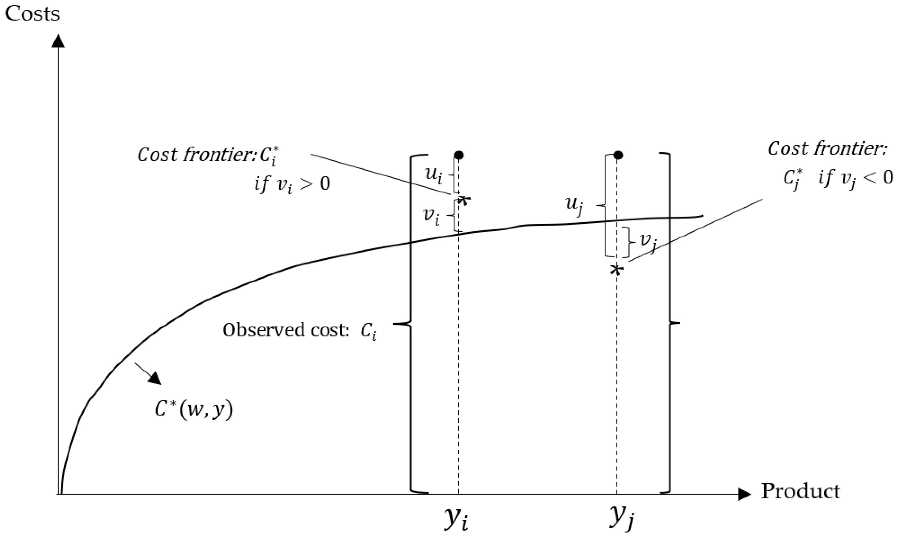
2.2. Theoretical Framework

The Stochastic Frontier Analysis method used for estimating the cost frontier of shrimp fishing companies in Mexico is based on the assumption that they aim to achieve the highest catch level at the lowest cost. According to the input-oriented technical inefficiency approach, a company is technically inefficient if it uses more inputs than those needed to achieve a certain catch level; thus, costs above the minimum efficient cost are due to input overuse. The approach used in this work followed the one developed by Meeusen and van den Broeck [10] and Kuenzle [38] adapted to the fisheries sector. Figure 5 shows the stochastic frontier of costs for two shrimp fishing companies with different catch levels.

Figure 5 shows two catch levels for shrimp fishing companies $i$ and $j$. Company $i$ has a catch level given by $y_i$ with an observed cost level given by $C_i$. $C^{\mathrm{*}}\left(w,y\right)$ is the deterministic cost function, where $w$ corresponds to an input price vector. Since company $i$ faces an unfavorable environmental condition negatively affecting the shrimp fishery yield (i.e., catch), the error component, $v_i,$ is positive, with higher production costs than those under favorable fishing environmental conditions, i.e., the value corresponding to the deterministic cost function. $u_i$ represents the deviation of company $i$ from the minimum cost frontier. A positive $u_i$ value means that the company has cost-inefficient production since it could achieve the same production at a lower cost. However, given that company $i$ cannot influence the value of $v_i$, measuring the deviation of efficiency costs relative to the deterministic cost function would be misleading. Company $j$ has a catch level given by $y_j$ with a production cost level given by $C_j$. Since $v_j$ is below the deterministic cost function, $v_j$ is negative. This implies that company $j$ faces favorable environmental conditions positively affecting the shrimp fishery yield, which reduces the frontier cost $C_j^{*}$. Nevertheless, company $j$ operates at a higher cost-inefficiency level $u$ than company $i,$ $u_i<u_j$, as $u$ measures the observed cost deviations relative to the frontier cost. However, cost inefficiency is a relative measure because company $j$ records catch levels far higher than company $i$, resulting from a greater fishing effort and, therefore, higher costs.

According to Kumbhakar et al. [39], the cost function can be expressed as follows:

$$C^{*}\left(w,y\right)=\sum _j{w}_j{x}_j{e}^{-u}$$

(1)

where $C^{*}\left(·\right)$ is the frontier cost function that produces the minimum cost, given the input price vector $w_j$, the quantity of inputs used $x_j$, and the observed production level. The cost minimization issue for companies under the input-oriented technical inefficiency approach can be expressed as follows:

$${}_{\left\{x_j{e}^{-u}\right\}}{}^{min}{w}^{\prime }x{e}^{-u}subject to:y=f\left(x{e}^{-u}\right)$$

(2)

The minimum cost $w^{\prime }x{e}^{-u}$ could be lower than the current cost $w^{\prime }x$, and technical inefficiency $u$ would indicate the percentage of overuse of all inputs needed to achieve the output level $y$. Alternatively, it could be interpreted as the percentage of use of all inputs that could be reduced without lowering the production level $y$. The observed cost $C^o$ of a company is expressed as follows:

$$C^o=\sum _j{w}_j{x}_j=C^{*}exp\left(u\right)$$

(3)

Transforming the previous expression to natural logarithms yields the following:

$$ln{C}^o=ln{C}^{*}\left(w,y\right)+u$$

(4)

The above equation shows that the natural logarithm of the observed cost $ln{C}^o$ increases along with $u$ because all inputs are overused. Following [8], the efficiency index specific to each company can be estimated as the ratio between the minimum cost $C^{*}$ and the observed cost $C^o$:

$$exp\left(-u\right)=\frac{C^{*}}{C^O}$$

(5)

When the restriction $u\ge 0$ is imposed, $exp\left(-u\right)$ takes values between 0 and 1.

2.3. Data Description

As mentioned above, information from two sources was used: (1) aquaculture and fisheries statistics yearbooks for the years 2003, 2008, 2013, and 2018 published by the Comisión Nacional de Acuicultura y Pesca (National Commission of Aquaculture and Fisheries; CONAPESCA, in Spanish) [3,4,5,6] and (2) economic censuses for the years 2003, 2008, 2013, and 2018 published by INEGI [34,35,36,37]. CONAPESCA data correspond to records of arrival notices of shrimp fishing vessels, while INEGI data correspond to census with coverage of all shrimp fishing economic units in Mexico. The data consist of the arrival location of the vessels, catches, costs, sales, and characteristics of the vessels.

Information concerning offshore and inshore shrimp catches (tons of live weight), and the number of offshore industrial vessels in each state was obtained from aquaculture and fishing statistics yearbooks. Information was obtained from economic censuses on the number of shrimp fishing companies by state, total costs (in millions of pesos), number of workers hired, expenditure on staff wages and salaries (in millions of pesos), gross fixed capital formation (in millions of pesos), and costs for fuel, lubricants, and energy consumption. Gross fixed capital formation was used as a variable that represents the value of vessels, refrigeration systems to preserve catches, engine power, navigation equipment, communication, eco-detection and satellite location, and fishing gear and capture methods. Variables with values in millions of pesos for each census year were deflated by the Producer Price Index (INPP), base June 2012 = 100 [40]. The prices of inputs per ton of shrimp catch (live weight) were calculated with the deflated economic variables, while information on subsidies was obtained from CONAPESCA [3,4,5,6].

Table 2. Description of variables.

Variable	Description	Unit
$Y$	Shrimp catch, live weight	Tons
$C$	Cost per ton of shrimp	$ MXN
$LP$	Labor price per ton of shrimp	$ MXN
$KP$	Capital price per ton of shrimp	$ MXN
$FP$	Fuel price per ton of shrimp	$ MXN
$Ln \left(Y\right)$	Natural log of shrimp catch, live weight	Log
$Ln \left(C\right)$	Natural log of cost per ton of shrimp	Log
$Ln \left(LP\right)$	Natural log of labor price per ton of shrimp	Log
$Ln \left(KP\right)$	Natural log of capital price per ton of shrimp	Log
$Ln \left(FP\right)$	Natural log of fuel price per ton of shrimp
$\frac{Ln \left(C\right)}{Ln \left(KP\right)}$	Normalized cost per ton of shrimp (cost/capital price)	Log
$\frac{Ln \left(LP\right)}{Ln \left(KP\right)}$	Normalized labor price (labor price/capital price)	Log
$\frac{Ln \left(FP\right)}{Ln \left(KP\right)}$	Normalized fuel price (fuel price/capital price)	Log
$Subsidies$	Liters of fuel subsidized to shrimp fishing companies by state	Percentage share

shows a detailed description of the variables.

Table 3. Descriptive statistics.

Variable	Mean	Std. Dev.	Min.	Max.	Obs.
$Y$	5841.83	8460.44	0	31,314.12	48
$C$	106,854.6	547,000.5	6.80	3,562,052	42
$LP$	73,996.66	386,858.1	759.88	2,518,768.0	42
$KP$	10,876.15	66,465.12	0.00	431,301.0	42
$FP$	27,056.89	108,369.6	2.38	704,702.2	42
$Ln \left(Y\right)$	7.48	1.94	0.43	10.35	42
$Ln \left(C\right)$	7.43	3.69	1.92	15.08	42
$Ln \left(LP\right)$	9.06	1.46	6.63	14.74	42
$Ln \left(KP\right)$	3.64	3.85	−6.488	12.97	42
$Ln \left(FP\right)$	6.65	3.60	0.87	13.46	42
$\frac{Ln \left(C\right)}{Ln \left(KP\right)}$	−0.28	18.44	−95.31	53.71	42
$\frac{Ln \left(LP\right)}{Ln \left(KP\right)}$	−2.90	45.99	−234.81	123.91	42
$\frac{Ln \left(FP\right)}{Ln \left(KP\right)}$	−0.08	16.04	−81.86	48.80	42
$Subsidies$	8.33	12.18	2	50	48

shows the descriptive statistics of the variables in tons and Mexican pesos, values in logarithms, and normalized values by dividing each variable by the price of capital.

2.4. Model Specification

Cost inefficiencies were estimated using three models. The first was the method proposed by Aigner et al. [9], which consists of a pooled frontier model estimated by maximum likelihood according to the following expression:

$$\frac{ln\left(C_{it}\right)}{ln\left({KP}_{it}\right)}=\alpha +{\beta }_Y\mathit{ln}\hspace{0.17em}{Y}_{it}+{\beta }_{PL}\frac{ln\left({LP}_{it}\right)}{ln\left({KP}_{it}\right)}+{\beta }_{PF}\frac{ln\left({FP}_{it}\right)}{ln\left({KP}_{it}\right)}+v_{it}-u_{it}$$

where index $i=\mathrm{1,2},\dots ,n$ indicates $n$ fishing representative units (FRUs), one per state, resulting in twelve, and $t=\mathrm{1,2},\dots ,T$ denotes the periods at which each FRU is observed, with four periods: 2003, 2008, 2003, and 2019. The dependent variable $\frac{ln\left(C_{it}\right)}{ln\left({KP}_{it}\right)}$ is the natural logarithm of the total cost per ton divided by the price of capital input, the same applied to the prices of labor and fuel input, thereby imposing the condition of homogeneity in prices. $\frac{ln\left({LP}_{it}\right)}{ln\left({KP}_{it}\right)}$ and $\frac{ln\left({FP}_{it}\right)}{ln\left({KP}_{it}\right)}$ are the natural logarithms of the normalized prices of labor and fuel inputs. ${\epsilon }_{it}$ is the term error composed of two parts: a stochastic error $v_{it}~iidN\left(0,{\sigma }_v^2\right)$ and a non-negative one-sided disturbance that captures the effect of inefficiency $u_{it}~iid{N}^{+}\left(\mu ,{\sigma }_u^2\right)$ and ${\epsilon }_{it}=v_{it}+u_{it}$.

The main limitation of the Pooled frontier model is that it does not allow capturing any specific effect of the FRU, so it does not distinguish between cost inefficiency and unobserved heterogeneity. To overcome this limitation, a True Fixed Effects (TFE) model was estimated, proposed by Greene [7,41]. This model treats time-invariant fixed effects specific for ${\alpha }_i$ and time-variable inefficiency $u_{it}$ separately, allowing for distinguishing between unobserved heterogeneity and inefficiency. The estimate with the TFE model allows for obtaining information on the transient component of efficiency. The first estimated model is

$$\frac{ln\left(C_{it}\right)}{ln\left({KP}_{it}\right)}={\alpha }_i+{\beta }_Y\mathit{ln}\hspace{0.17em}{Y}_{it}+{\beta }_{PL}\frac{ln\left({LP}_{it}\right)}{ln\left({KP}_{it}\right)}+{\beta }_{PF}\frac{ln\left({FP}_{it}\right)}{ln\left({KP}_{it}\right)}+v_{it}-u_{it}$$

(6)

where index $i=\mathrm{1,2},\dots ,n$ indicates $n$ fishing representative units (FRUs), and $t=\mathrm{1,2},\dots ,T$ denotes the periods at which each FRU is observed. $\frac{ln\left(C_{it}\right)}{ln\left({KP}_{it}\right)}$ is the natural logarithm of the total cost per ton normalized. ${\alpha }_i$ represents the FRU-specific fixed effects. $\frac{ln\left({LP}_{it}\right)}{ln\left({KP}_{it}\right)}$ and $\frac{ln\left({FP}_{it}\right)}{ln\left({KP}_{it}\right)}$ are the natural logarithms of the normalized prices of labor and fuel inputs. ${\epsilon }_{it}$ is the term error composed of two parts: a stochastic error $v_{it}~iidN\left(0,{\sigma }_v^2\right)$ and a non-negative one-sided disturbance that captures the effect of inefficiency $u_{it}~iid{N}^{+}\left(\mu ,{\sigma }_u^2\right)$ and ${\epsilon }_{it}=v_{it}+u_{it}$. The estimation of this model implies assuming the assumption of persistent inefficiency close to zero or null. If there is persistent inefficiency, it will be completely absorbed in the individual-specific constant term. Another characteristic of the TFE model is that it allows a correlation between heterogeneity and explicatory variables and therefore provides unbiased estimates of the parameters $\beta$. However, in the presence of factors that generate persistent inefficiency, such as predetermined environmental conditions of production that affect the availability and quality of resources, it would not be possible to include time-invariant variables, due to the perfect multicollinearity (Addo and Salhofer [42]).

Due to the above limitations, Colombi et al. [43] proposed an alternative econometric specification which they labeled as the “Generalized True Random Effects Model” (GTRE); subsequently, Colombi et al. [44], Tsionas and Kumbhakar [45], and Kumbhakar et al. [8] developed models that allow estimating persistent and transient inefficiencies through a four-way decomposition of the error term into ${\epsilon }_{it}=w_i-h_i+v_{it}-u_{it}$, where $w_i-h_i$ represents a permanent heterogeneous frontier effect while $v_{it}-u_{it}$ represents a transitory component (Sickles and Zelenyuk [46]). With the purpose of estimating persistent inefficiencies, we apply the four-error component model using the multi-step technique proposed by Kumbhakar et al. [8]:

$$\begin{gathered} \frac{ln\left(C_{it}\right)}{ln\left({KP}_{it}\right)}={\alpha }_0+{\beta }_Y\mathit{ln}\hspace{0.17em}{Y}_{it}+{\beta }_{PL}l\frac{ln\left({LP}_{it}\right)}{ln\left({KP}_{it}\right)}+{\beta }_{PF}\frac{ln\left({FP}_{it}\right)}{ln\left({KP}_{it}\right)}+{\mu }_i-{\eta }_i+v_{it}-u_{it}; \\ {v}_{it}~iidN\left(0,{\sigma }_v^2\right);u_{it}~iid{N}^{+}\left(\mu ,{\sigma }_u^2\right);{\epsilon }_{it}=v_{it}+u_{it} \end{gathered}$$

where $u_{it}~N^{+}\left(0,{\sigma }_u^2\right)$ corresponds to the component of persistent inefficiency (long run); ${\eta }_i~N^{+}\left(0,{\sigma }_{\eta }^2\right)$ represents the component of transient inefficiency that varies randomly between companies (Short-Run). ${\mu }_i$ is a component that captures the heterogeneity of the companies, and $v_{it}~N\left(0,{\sigma }_v^2\right)$ is a random component. Cost inefficiency can be expressed in terms of the cost inefficiency score:

$$\frac{C_{it}}{C_{it}^F}=E\left(u_{it}|{\epsilon }_{it}\right)$$

(7)

where $C_{it}$ is the observed cost and $C_{it}^F$ is the frontier cost or minimum cost. The inefficiencies and efficiencies specific to each FRU $i$ in the period $t$ were obtained following the procedure by Jondrow et al. [47], calculated from the expected $u_{it}$ value that depends on the compound error ${\epsilon }_{it}$ of the model, assuming that the density function of $\left(u_{it}|{\epsilon }_{it}\right)$ is $N^{+}({\mu }_{*i},{\sigma }_{*}^2)$, where ${\mu }_{*i}=\frac{-{\sigma }_u^2{\epsilon }_i}{{\sigma }_v^2+{\sigma }_u^2}$ and ${\sigma }_{*}^2=\frac{{\sigma }_v^2{\sigma }_u^2}{{\sigma }_v^2+{\sigma }_u^2}$. This estimates the specific values of inefficiencies $E\left(u_{it}|{\epsilon }_{it}\right)$ and efficiencies $E\left[exp\left(-u_{it}\right)|{\epsilon }_{it}\right]$ of shrimp fishing companies. The specific cost-efficiency values lie within $0\ge E\left[exp\left(-u_{it}\right)|{\epsilon }_{it}\right]\le 1$, where a score of 1 indicates that companies are on the minimum cost-efficient frontier, while those with a lower score have deviations from the cost-efficient frontier.

We contrasted the effects of the fuel subsidies on the inefficiencies of companies. To this end, the parameterization approach was used, assuming that the mean and variance of the pretruncated distribution of inefficiencies are linear functions of the exogenous variables $u_{it}={Subsidies}_{it}^{\prime }\delta$; ${\sigma }_{it}^2=\mathrm{e}\mathrm{x}\mathrm{p}\hspace{0.17em}\left({Subsidies}_{it}^{\prime }w\right)$, where $Subsidies$ is the percentage share of subsidies by companies of each state, and $\delta$ and $w$ represent the coefficients to compare the relationship following Kumbhakar [48], Reifschneider and Stevenson [49], Huang and Liu [50], Battese and Coelli [51], Wang [52], and Kumbhakar et al. [8]. In addition, we estimated the marginal effect of the increase in the share of fuel subsidies on cost inefficiencies. $\left[\frac{\partial E\left(u_{it}|{\epsilon }_{it}\right)}{\partial {Subsidies}_{it}}\right],$ according to Sun and Kumbhakar [53].

3. Results

Table 4. Estimation results of the cost frontier function.

$\mathbf{Normalized} \mathbf{Cos}\mathbf{t} \mathbf{Per} \mathbf{Ton} \mathbf{of} \mathbf{Shrimp}: \frac{\mathit{L}\mathit{n}\left(\mathit{C}\right)}{\mathit{L}\mathit{n}\left(\mathit{K}\mathit{P}\right)}$	Pooled	$\mathit{T}\mathit{F}\mathit{E}~\left[\mathit{T}\mathit{N}\left(\mathit{\mu },\mathit{\sigma }\right)\right]$	1st Step FE Kumbhakar et al. [8]	2nd Step Kumbhakar et al. [8]	3rd Step Kumbhakar et al. [8]
Shrimp catch: $\mathit{ln}\hspace{0.17em}\left(Y\right)$	−0.04	−0.11 ***	−0.05
	(0.03)	(0.00001)	(0.03)
Normalized fuel price: $\frac{Ln\left(FP\right)}{Ln\left(KP\right)}$	0.97 ***	0.75 ***	0.96 ***
	(0.03)	(0.000004)	(0.03)
Normalized labor price: $\frac{Ln\left(LP\right)}{Ln\left(KP\right)}$	0.06 ***	0.13 ***	0.07 ***
	(0.01)	(0.000001)	(0.01)
Year	0.01	0.02 ***	0.02 **
	(0.01)	(0.00005)	(0.01)
Constant	−21.35		−40.82 **	3.38 × 10−18 ***	0.31 ***
	(20.11)		(20.41)	(7.49 × 10−19)	(0.08)
$\mu \left(TFE:subsidies\right)$		−1.08 ***
		(0.31)
${\sigma }_u\left(TFE:subsidies\right)$		0.09 ***		−80.5	−1.85 ***
		(0.01)			(0.50)
${\sigma }_v\left(TFE:subsidies\right)$		−32.85		−81.95 ***	−2.82 ***
		(228.85)		(0.63)	(0.40)
${\sigma }_u^2$	0.43	1.9		3.32 × 10−18	0.40
${\sigma }_v^2$	0.22	7.00 × 10−8		1.6 × 10−18	0.24
$\lambda =\raisebox{1ex}{${\sigma }_u$}\!\left/ \!\raisebox{-1ex}{${\sigma }_v$}\right.$	2.00	2.08			1.621424
$\gamma =\raisebox{1ex}{${\sigma }^2$}\!\left/ \!\raisebox{-1ex}{${\sigma }_u^2$}\right.$	0.79	0.99		0.81	0.74
Log-likelihood	−13.42	−5.11		1657.64	−13.99
$Wald{chi}^2$	3.63	3.84 × 1012			13.64
$Prob>{chi}^2$	0.03	0.00			0.00

Note: ** p < 0.05; *** p < 0.01.

shows the results of the Pooled and True Fixed Effects stochastic cost frontier models and the three-step model developed by Kumbhakar et al. [8].

Since the variables are expressed in logarithmic terms, the coefficients can be interpreted as elasticities. The coefficients of the shrimp catch variable were negative in the three estimated models. However, of these, only the estimate using the TFE model was statistically significant (−0.11) at 99% confidence, indicating that on average, a 10% increase in the catch reduces the cost by 1.1%, ceteris paribus. Following the development of Christensen and Greene [54], who consider the presence of scale economies (ES), from one unit minus the elasticity of the cost with respect to the catch (for this study), where a positive value indicates economies of scale and a negative value indicates diseconomies of scale, it was found that the sector experienced ES during the study period: $ES=1-\partial lnC/\partial lnY=1-\left(-0.11\right)=1.11$.

The coefficients of the labor and fuel price variables were positive and statistically significant in the three models $\left(p<0.001\right)$, suggesting compliance with the monotonicity condition in the cost function. The fuel price coefficients were of greater magnitude in the Pooled (0.97) and Random Effects (0.96) models, and in the first step of Kumbhakar et al.’s model [8], with respect to the coefficient estimated in the TFE model (0.75). Considering the coefficient obtained in the TFE model, the cost elasticity relative to the fuel input was inelastic (0.75), indicating that fishing effort has a major effect on the operation costs of the shrimp fishing fleets. In terms of elasticity, the coefficient of fuel price indicates that a 1% increase in fuel use, ceteris paribus, translates into a 0.75% increase in operating costs. This result is in accordance with what was expected, with respect to the fact that the shrimp fishery is intensive in fuels; that is, the percentage change in the price of fuel has a greater influence on cost than other inputs. The coefficient of the labor price variable was higher in the TFE model (0.13) than in the Pooled (0.06) and Random Effects (0.07) models, revealing that although labor is important in the fishery, the percentage change in its price has less influence on cost than the fuel input. Considering the results of the TFE model, a 1% increase in labor, ceteris paribus, increases costs by 0.13%. The price elasticity of capital was 0.12 $\left[1-\left({\beta }_{LP}+{\beta }_{FP}\right)\right]$, indicating that a 1% increase in this input, ceteris paribus, increases costs by 0.12%. The coefficients of the year variable were positive (0.02) and statistically significant in the TFE and random effects models (first step of Kumbhakar et al. [8]), indicating that costs per ton of shrimp caught increased by 2% in real terms during the study period.

In the case of the TFE model, the coefficient of the subsidy variable for $\mu$ was negative and statistically significant $\left(p<0.001\right)$. The subsidy coefficients for ${\sigma }_u$ were only statically significant $\left(p<0.001\right)$ in the TFE and Kumbhakar et al. [8] models of transient inefficiencies. The coefficients of the variable subsidies for ${\sigma }_v$ were statistically significant $\left(p<0.001\right)$ only in the model of Kumbhakar et al. [8]. It is important to note that the $\mu$ and ${\sigma }_u$ coefficients obtained from the estimated TFE model, assuming a truncated normal distribution with the variable subsidies as an exogenous determinant of the inefficiencies of shrimp fishing companies by state, are not directly interpretable, so it is necessary to estimate the effect margins on the unconditional expectation of $u$, $E\left(u\right)$, and the unconditional variance of $u$, $V\left(u\right)$.

The values obtained from $\gamma$ suggest that between 71% and 99% of the deviations from the minimum efficient cost frontier are due to inefficient shrimp fishing economic units and the percentage difference to the stochastic component. To confirm the above, we assessed the statistical significance of the parameters $\gamma$ using the likelihood ratio test $-2\left[L\left(H_0\right)-L\left(H_1\right)\right]\approx {\chi }_{k-1}^2$, where $L\left(H_0\right)$ is the logarithm of the likelihood function at the maximum for the estimated Generalized Linear Model (GLM), and $L\left(H_1\right)$ is the logarithm of the likelihood function at the maximum for the estimated models. The values of $-2\left[L\left(H_0\right)-L\left(H_1\right)\right]$ were 3.62 (Pooled), 20.24 (TFE), 3345.75 (second step to estimate persistent inefficiencies using Kumbhakar et al.’s model [8]), and 2.5 (third step to estimate transient inefficiencies using Kumbhakar et al.’s model [8]), and the theoretical value of the distribution ${\chi }_{k-1}^2$ with an alpha of 0.05 was 2.70. Therefore, the null hypothesis that the stochastic frontier models used (Pooled, TFE, and the second step of Kumbhakar et al.’s model [8] to estimate persistent inefficiencies) are not appropriate is rejected. For the model of time-varying inefficiencies, the null hypothesis is rejected with a level of significance of 0.10. Cost inefficiencies were estimated following the procedure developed by Jondrow et al. [47].

Table 5. Statistical summary of estimated cost-inefficiency scores.

Efficiency Scores	Pooled	TFE	Kumbhakar et al. [8]
	Overall	Transient	Time-Varying
Mean	0.64	0.75	0.69
Std. Dev.	0.31	0.29	0.19
Min.	0.03	0.05	−0.08
Max.	0.99	0.99	0.92

shows a statistical summary of the estimated cost-inefficiency scores.

The mean of the cost efficiencies in the three models was found to be within the range of 0.64 to 0.75. In the case of the True Fixed Effects model, when estimating transient inefficiencies, it was found that on average, the shrimp fishing fleet in Mexico registered an efficiency of 0.75. This indicates that the shrimp fishing fleet could lower costs by 25% without reducing the current catch levels. That is, on average, the difference between the minimum possible cost per ton of shrimp captured from the most efficient FRUs and the cost per ton of the rest of the FRU was 25%. The FRU could reduce their costs through the optimal use of inputs, given the environmental conditions. Transient cost inefficiency shows that an FRU, given the price of inputs, uses a certain amount of inputs to catch a ton of shrimp, but the cost per ton of shrimp is higher than another FRU that uses the same amount of inputs. The above controls for unobserved heterogeneity attributable to the specific characteristics of the FRU.

Figure 6 shows technical efficiencies by marine region obtained from the True Fixed Effects model.

Companies with shrimp fleets in the Gulf of California and South Pacific presented higher cost inefficiencies compared to companies that operate in the Gulf of Mexico, with mean inefficiency values of 0.31 and 0.13, respectively. To analyze the effects of subsidies for fuels such as gasoline and diesel, the marginal effects of the share of liters of fuel received on cost inefficiencies were estimated.

Table 6. Descriptive statistics of the marginal effects of subsidies on inefficiency.

Variable	Mean	Std. Dev.	Min.	Max.
$\frac{\partial E\left(u_{it}|{\epsilon }_{it}\right)}{\partial {Subsidies}_{it}}$	−0.17	0.04	−0.21	−0.03
$\frac{\partial {\sigma }_{E\left(u_{it}|{\epsilon }_{it}\right)}^2}{\partial {Subsidies}_{it}}$	−0.10	0.20	−0.30	0.75

shows the marginal effect of the natural logarithm of the variable subsidies on the mean $E\left(u_{it}|{\epsilon }_{it}\right)$ and variance ${\sigma }_{E\left(u_{it}|{\epsilon }_{it}\right)}^2$ of the inefficiency.

The mean and variance of the marginal effects of the subsidies on technical inefficiencies were negative, indicating that increases in the liters of subsidized fuel contribute to reducing cost inefficiencies. This subsidy also contributed to reducing the variability of inefficiencies. Figure 7 graphically shows the marginal effects of the participation of fuel subsidies on cost inefficiencies of shrimp fishing companies in Mexico during the period from 2003 to 2018.

Figure 7 shows that fuel subsidies led to a reduction in cost inefficiencies. The greatest marginal effects in absolute terms were reached in fishing companies located in states that received 20% of the total liters of subsidized fuel, while fishing fleets located in states with a share of subsidized fuel greater than 20% showed a decrease in inefficiencies; however, this effect decreased as the percentage share of subsidized fuel increased. Compliance with the monotonicity condition was validated by calculating partial derivatives of input prices $\left(LP,KP y FP\right)$ and catch $\left(Y\right)$ relative to the cost.

4. Discussion

The technical efficiency levels reported in previous studies are not directly comparable. However, the factors affecting catches, costs, and technical efficiency can be analyzed through the magnitude, sign, and statistical significance of the estimated coefficients in the production and inefficiency models. In this sense, the signs of the coefficients representing the elasticity of costs relative to the use of inputs were consistent with economic theory. In this study, the cost elasticity relative to the labor input (crew size) was 0.13, close to the 0.28 figure reported by Jamnia et al. [25]; lower than 0.40 reported by Quijano et al. [26], Dian et al. [27], and Agar et al. [30]; and lower than 0.42 reported by Esmaeili [22]. The fuel price elasticity of 0.75 (cost per ton) of the TFE model was much higher than 0.27 found by Kompas et al. [17] for the shrimp fishing fleet in northern Australia during the period 1990–1996. These differences indicate that the shrimp fishery in the Mexican Pacific was more fuel-intensive than the shrimp fishery in northern Australia. Regarding fishing inefficiency, in this study, a transitory cost inefficiency of 0.31 was found for the Mexican Pacific shrimp fishing fleet, greater than that reported by Cabrera and González [23], who found an average output-oriented technical inefficiency of 0.21 for the fishing fleet of the upper Gulf of California, Mexico, for the period 1990–1993. This study used the fixed capital formation value, in contrast with previous studies using gross registered tonnage, engine horsepower, and vessel length, so that cost elasticity relative to capital is not directly comparable to other reports in the empirical literature.

Regarding the factors that affect the cost inefficiencies of shrimp fishing companies in this study, we used the percentage share of subsidized fuel to measure its impact on cost inefficiencies. The results reported herein indicate that increases in the fuel subsidy favor a reduction in cost inefficiencies in the shrimp fishing industry. However, this effect is less for fishing fleets located in states that concentrate more than 20% of the subsidized fuel. This result is consistent with the findings reported by Dağtekin et al. [31] regarding the fact that subsidies favor the technical efficiency of artisanal fishing. Likewise, the findings found in this study are in line with those reported by N’Souvi et al. [32] in the sense that the subsidies reduce the inefficiencies of the pelagic trawl fishery. A contribution of this study to the literature was the measurement of the effect of the fuel subsidy of shrimp fishing companies through the marginal effect of the percentage share of liters of subsidized fuel, highlighting that the greatest effects are reached in states that concentrate 20% of subsidies. This result indicates that managers and captains minimized operating costs in terms of fuel spending and the liters of subsidized gasoline or diesel.

This study has a spatial and temporal scope on the cost efficiency of the shrimp fishing sector in Mexico from 2003 to 2018. The main limitation of the study was the number of observations. Nevertheless, it was possible to estimate the three-stage model of Kumbhakar et al. [8], which allowed obtaining persistent and time-varying inefficiencies. The True Fixed Effects model was also estimated, through which the transient inefficiencies were obtained. Regarding the results obtained, it was found that by using the three-stage model of Kumbhakar et al. [8], the persistent inefficiencies were very small, close to zero. The score of the time-varying inefficiencies is not robust, because in the likelihood ratio test, the null hypothesis was not rejected at 95% confidence (it was rejected at 90% confidence). Due to the above, the TFE model was selected to analyze the transient cost inefficiencies of the shrimp fishing industry during the period from 2003 to 2018. Another limitation is the lack of information on the available shrimp biomass at a compatible national level for the years analyzed in this study.

5. Conclusions

To date, this study is the first to analyze the cost inefficiencies of the shrimp fisheries in Mexico at the national level using publicly available longitudinal data. From the estimation of a true fixed effects model, an average transient cost inefficiency of 0.25 was obtained, indicating that on average, FRUs could reduce the cost per ton of shrimp by 25%.

On overage, fishing companies in the Gulf of California and South Pacific were less efficient (0.31) than those operating in the Gulf of Mexico (0.13). As for the intensity of production inputs, we found that the shrimp fishery is intensive in the use of fuels (0.75) and, to a lesser extent, in the use of labor (0.13) and capital (0.12). From the analysis of the marginal effects of the fuel subsidy on cost inefficiencies, it was highlighted that the greatest marginal effect on the reduction in inefficiencies is reached at a level of 20% of the total subsidized fuel. This has major implications for the design of subsidy policy programs for the shrimp fishery sector.

References

1. CONAPESCA. Anuario Estadístico de Acuacultura y Pesca; Comisión Nacional de Pesca: Mazatlán, México, 2019. Available online: https://www.gob.mx/conapesca/documentos/anuario-estadistico-de-acuacultura-y-pesca (accessed on 12 January 2023).
2. Aranceta-Garza, F.; Arreguín-Sánchez, F.; Seijo, J.C.; Ponce-Díaz, G.; Lluch-Cota, D.; del Monte-Luna, P. Determination of catchability-at-age for the Mexican Pacific shrimp fishery in the southern Gulf of California. Reg. Stud. Mar. Sci. 2020, 33, 100967. [Google Scholar] [CrossRef]
3. CONAPESCA. Anuario Estadístico de Acuacultura y Pesca; Comisión Nacional de Pesca: Mazatlán, México, 2003. Available online: https://www.gob.mx/conapesca/documentos/anuario-estadistico-de-acuacultura-y-pesca (accessed on 12 January 2023).
4. CONAPESCA. Anuario Estadístico de Acuacultura y Pesca; Comisión Nacional de Pesca: Mazatlán, México, 2008. Available online: https://www.gob.mx/conapesca/documentos/anuario-estadistico-de-acuacultura-y-pesca (accessed on 12 January 2023).
5. CONAPESCA. Anuario Estadístico de Acuacultura y Pesca; Comisión Nacional de Pesca: Mazatlán, México, 2013. Available online: https://www.gob.mx/conapesca/documentos/anuario-estadistico-de-acuacultura-y-pesca (accessed on 12 January 2023).
6. CONAPESCA. Anuario Estadístico de Acuacultura y Pesca; Comisión Nacional de Pesca: Mazatlán, México, 2018. Available online: https://www.gob.mx/conapesca/documentos/anuario-estadistico-de-acuacultura-y-pesca (accessed on 12 January 2023).
7. Greene, W.H. Fixed and random effects in stochastic frontier models. J. Product. Anal. 2005, 23, 7–32. [Google Scholar] [CrossRef]
8. Kumbhakar, S.C.; Lien, G.; Hardaker, B.J. Technical efficiency in competing panel data models: A study of Norwegian farming. J. Product. Anal. 2014, 41, 321–337. [Google Scholar] [CrossRef]
9. Aigner, D.; Lovell, C.A.K.; Schmidt, P. Formulation and estimation of stochastic frontier production function models. J. Econom. 1977, 6, 21–37. [Google Scholar] [CrossRef]
10. Meeusen, W.; van den Broeck, J. Efficiency Estimation from Cobb-Douglas Production Functions with Composed Error. Int. Econ. Rev. 1977, 18, 435–444. [Google Scholar] [CrossRef]
11. Kirkley, J.; Squires, D.; Strand, I. Assessing technical efficiency in commercial fisheries: The mid-Atlantic Sea scallop fishery. Am. J. Agric. Econ. 1995, 77, 686–697. [Google Scholar] [CrossRef]
12. Sharma, K.; Leung, P. Technical efficiency of the longline fishery in Hawaii: An application of a stochastic production frontier. Mar. Resour. Econ. 1999, 13, 259–274. [Google Scholar] [CrossRef]
13. Eggert, H. Technical Efficiency in the Swedish Trawl Fishery for Norway Lobster. In Microbehavior and Macroresults, Proceedings of the Tenth Biennial Conference of the International Institute of Fisheries Economics and Trade, Corvallis, OR, USA, 10–14 July 2000; Johnston, R.S., Shriver, A.L., Eds.; IIFET: Corvallis, OR, USA, 2001. [Google Scholar]
14. Pacoe, S.; Cogan, L. The Contribution of unmeasurable inputs to fisheries production: An analysis of Fishing Vessels in the English Channel. Am. J. Agric. Econ. 2002, 84, 585–597. [Google Scholar]
15. Fousekis, P.; Klonaris, S. Technical efficiency determination for fisheries: A study of trammel netters in Greece. Fish. Res. 2003, 63, 85–95. [Google Scholar] [CrossRef]
16. Herrero, I.; Pascoe, S. Value versus Volume in the catch of the Spanish South-Atlantic trawl fishery. J. Agric. Econ. 2003, 54, 325–341. [Google Scholar] [CrossRef]
17. Kompas, T.; Che, T.N.; Grafton, Q. Technical efficiency effects of input controls: Evidence from Australia’s banana prawn fishery. Appl. Econ. 2004, 36, 1631–1641. [Google Scholar] [CrossRef]
18. García del Hoyo, J.J.; Castilla, E.D.; Jiménez, T.R. Determination of technical efficiency of fisheries by stochastic frontier models: A case on the Gulf of Cádiz (Spain). ICES J. Mar. Sci. 2004, 61, 416–421. [Google Scholar] [CrossRef]
19. Tingley, D.; Pascoe, S.; Cogan, L. Factor affecting technical efficiency in fisheries: Stochastic production frontier versus data envelopment analysis approaches. Fish. Res. 2005, 73, 363–376. [Google Scholar] [CrossRef]
20. Herrero, I. Different approaches to efficiency to analysis. An application to the Spanish trawl fleet operating in Moroccan waters. Eur. J. Oper. Res. 2005, 167, 257–271. [Google Scholar] [CrossRef]
21. Jeon, Y.; Ishak, H.O.; Kuperan, K.; Squires, D.; Susilowati, I. Developing country fisheries and technical efficiency: The Java Sea purse seine fishery. Appl. Econ. 2006, 38, 1541–1552. [Google Scholar] [CrossRef]
22. Esmaeili, A. Technical efficiency analysis for the Iranian fishery in the Persian Gulf. ICES J. Mar. Sci. 2006, 63, 1759–1764. [Google Scholar] [CrossRef]
23. Cabrera, H.R.; González, J.R. Manejo y Eficiencia en la pesquería del camarón del Alto Golfo de California. Estud. Soc. 2006, 14, 125–138. [Google Scholar]
24. Chowdhury, N.K.; Kompas, T.; Kalirajan, K. Input and Quality Controls: A Stochastic Frontier Analysis of Bangladesh’s Industrial Trawl Fishery. In Proceedings of the AARES 54th Annual Conference, Adelaide, Australia, 10–12 February 2010; Australian Agricultural and Resource Economics Society: Adelaide, Australia, 2010; pp. 1–14. [Google Scholar]
25. Jamnia, A.R.; Mazloumzadeh, S.M.; Keijha, A.A. Estimate the technical efficiency of fishing vessels operating in Chabahar region, Southern Iran. J. Saudi Soc. Agric. Sci. 2015, 14, 26–32. [Google Scholar] [CrossRef]
26. Quijano, D.; Salas, S.; Monroy-García, C.; Velazquez-Abunader, I. Factors contributing to technical efficiency in a mixed fishery: Implications in buyback programs. Mar. Policy 2018, 94, 61–70. [Google Scholar] [CrossRef]
27. Dian, A.N.N.; Iskandar, D.D. Pekalongan Purse Seiners Fisheries Technical Efficiency Using Stochastic Frontier Panel Data. In IOP Conference Series: Earth and Environmental Science, Proceedings of the 4th International Conference on Tropical and Coastal Region Eco Development, Semarang, Indonesia, 30–31 October 2018; IOP Publishing: Bristol, UK, 2019; Volume 246, p. 012014. [Google Scholar]
28. Castilla, E.D.; García del Hoyo, J.J. Eficiencia técnica de pesquerías con heterogeneidad inobservada. Estud. Econ. Aplic. 2019, 37, 101–112. [Google Scholar] [CrossRef]
29. Nguyen-Anh, T.; Hoang-Duc, L.; Nguyen-Thi-Thuy, L.; Vy-Tienb, V.; Nguyen-Dinha, U.; To-Thea, N. Do intangible assets stimulate firm performance? Empircal evidence from Vietnamesse Agriculture, forestry and fishery small- and medium sized enterprises. J. Innov. Knowl. 2022, 7, 100194. [Google Scholar] [CrossRef]
30. Agar, J.; Horrace, C.W.; Parmeter, C.F. Overcapacity in Gulf of Mexico reef fish IFQ fisheries: 12 years after the adoption of IFQs. Environ. Resour. Econ. 2022, 82, 483–506. [Google Scholar] [CrossRef]
31. Dağtekin, M.; Uysal, O.; Candemir, S.; Genç, Y. Productive efficiency of the pelagic trawl fisheries in the Southern Black Sea. Reg. Stud. Mar. Sci. 2021, 45, 101853. [Google Scholar] [CrossRef]
32. N’Souvi, K.; Sun, C.; Rivero, Y.M. Development of marine small-scale fisheries in Togo: An examination of the efficiency of fishermen at the new fishing port of Lomé and the necessity of fisheries co-management. Aquac. Fish. 2023; in press. [Google Scholar] [CrossRef]
33. CONABIO. Sistema Nacional de Información sobre Biodiversidad de México. 2022. Available online: https://www.snib.mx/ (accessed on 3 February 2023).
34. INEGI. Censos Económicos. Mexico. 2004. Available online: https://www.inegi.org.mx/app/saic/default.html (accessed on 6 February 2023).
35. INEGI. Censos Económicos. Mexico. 2009. Available online: https://www.inegi.org.mx/app/saic/default.html (accessed on 6 February 2023).
36. INEGI. Censos Económicos. Mexico. 2014. Available online: https://www.inegi.org.mx/app/saic/default.html (accessed on 6 February 2023).
37. INEGI. Censos Económicos. Mexico. 2020. Available online: https://www.inegi.org.mx/app/saic/default.html (accessed on 6 February 2023).
38. Kuenzle, M. Cost Efficiency in Network Industries. Application of Stochastic Frontier Analysis. Ph.D. Thesis, Swiss Federal Institute of Technology, Zürich, Switzerland, 2005. Available online: https://www.research-collection.ethz.ch/handle/20.500.11850/53059 (accessed on 4 March 2023).
39. Kumbhakar, S.C.; Wang, H.; Horncastle, A.P. A Practitioner’s Guide to Stochastic Frontier Analysis Using Stata; Cambridge University Press: New York, NY, USA, 2015. [Google Scholar]
40. INEGI. Índice de Nacional de Precios; Instituto Nacional de Estadística y Geografía: Ciudad de México, México, 2019; Available online: https://www.inegi.org.mx/temas/inpp/ (accessed on 13 February 2023).
41. Greene, W.H. Reconsidering Heterogeneity in Panel Data Estimator of the Stochastic Frontier Model. J. Econom. 2005, 126, 269–303. [Google Scholar] [CrossRef]
42. Addo, F.; Salhofer, K. Transient and Persistent technical efficiency and its determinants: The case of crop farms in Austria. Appl. Econ. 2022, 54, 25. [Google Scholar] [CrossRef]
43. Colombi, R.; Martini, G.; Vittadini, G. A Stochastic Frontier Model with Short-Run and Long-Run Inefficiency Random Effects; Working Paper Series; Department of Economics and Technology Management, University of Bergamo: Bergamo, Italy, 2011. [Google Scholar]
44. Colombi, R.; Kumbhakar, S.C.; Martini, G.; Vittadini, G. Closed-Skew Normality in Stochastic Frontier with individual Effects and Long/Short-Run Efficiency. J. Product. Anal. 2014, 42, 123–136. [Google Scholar] [CrossRef]
45. Tsionas, E.G.; Kumbhakar, S.C. Firm Heterogeneity, Persisten and Transient Technical Inefficiency: A Generalized True Random-Effects Model. J. Appl. Econom. 2014, 29, 110–132. [Google Scholar] [CrossRef]
46. Sickles, R.C.; Zelenyuk, V. Measurement of Productivity and Efficiency. Theory and Practice; Cambridge University Press: Cambridge, UK, 2019. [Google Scholar]
47. Jondrow, J.; Lovell, C.A.K.; Materov, I.S.; Schmidt, P. On the estimation of technical inefficiency in the stochastic frontier production function model. J. Econom. 1982, 19, 233–238. [Google Scholar] [CrossRef]
48. Kumbhakar, S.C. The Measurement and Decomposition of Cost-Inefficiency: The Translog Cost System. Oxf. Econ. Pap. 1991, 43, 667–683. [Google Scholar] [CrossRef]
49. Reifschneider, D.; Stevenson, R. System Departures from the Frontier: A Framework for the Analysis of Firm Inefficiency. Int. Econ. Rev. 1991, 32, 715–723. [Google Scholar] [CrossRef]
50. Huang, C.; Liu, J.T. Estimation of a Non-Neutral Stochastic Frontier Production Function. J. Product. Anal. 1994, 7, 257–282. [Google Scholar] [CrossRef]
51. Battese, G.E.; Coelli, T.J. A Model for Technical Inefficiency Effects in a Stochastic Frontier Production Function for Panel Data. Empir. Econ. 1995, 20, 325–332. [Google Scholar] [CrossRef]
52. Wang, H.J. Heteroscedasticity and Non-Monotobic Efficiency Effects of a Stochastic Frontier Model. J. Product. Anal. 2002, 18, 241–253. [Google Scholar] [CrossRef]
53. Sun, K.; Kumbhakar, S.C. Semiparametric Smooth-Coefficient Stochastic Frontier Model. Econ. Lett. 2013, 120, 305–309. [Google Scholar] [CrossRef]
54. Christensen, L.R.; Greene, W.H. Economies of scale in U.S. Electric Power Generation. J. Polit. Econ. 1976, 84, 655–976. [Google Scholar] [CrossRef]
Figure 1. Spatial distribution of shrimp by species. Source: Own elaboration based on CONABIO’s National Information System on Biodiversity of Mexico [33].
Fishes 08 00472 g001
Figure 2. Tons of main shrimp species caught during the period 2006–2018.
Fishes 08 00472 g002
Figure 3. Shrimp catches by state, 2006–2018.
Fishes 08 00472 g003
Figure 4. Fuel subsidy distribution by state, during the period 2008–2018.
Fishes 08 00472 g004
Figure 5. Graphical illustration of stochastic frontier costs.
Fishes 08 00472 g005
Figure 6. Cost efficiencies by marine region: (a) kernel density by region; (b) boxplot by region.
Fishes 08 00472 g006
Figure 7. Marginal effect of subsidized fuel on inefficiency.
Fishes 08 00472 g007