Reproductive Success Dynamics Could Limit Precision in Close-Kin Mark–Recapture Abundance Estimation for Atlantic Goliath Grouper (Epinephelus itajara)

Abstract

Extra-Poisson variance in annual reproductive success can affect the precision of abundance estimates made using ‘close-kin’ mark–recapture procedures. However, empirical evaluation of that variance in natural marine populations can be daunting. Here, a scaling method was used to extend a discrete-time, age-structured model, facilitating investigation of annual and lifetime reproductive success dynamics in Epinephelus itajara. Life tables were synthesized from fishery assessment vital rates and life history measures. For model scaling, a precise empirical estimate of effective population size for the studied population was utilized as the independent variable, and model sensitivity to an informative range of adult abundance was evaluated. The potential for sex reversal to impact reproductive success dynamics was also investigated, albeit in the absence of selective fishing pressure and potential compensatory or depensatory responses. Close-kin relationships in a genetic sample of ~300 adults collected from spawning sites in the Florida Atlantic included numerous full-sibling pairs and multi-sibling families, which is unusual for long-lived, iteroparous marine populations with broadly dispersed larvae. The highly overdispersed reproductive success dynamics modeled for this population and its atypical kinship distribution could have ramifications for planned close-kin mark–recapture analyses. The low observed effective size also has conservation implications. Both issues warrant continued genetic monitoring.

1. Introduction

Because they can now be implemented at useful scales, genetic-based capture–mark–recapture, GCMR, and close-kin mark–recapture, CKMR, are growing in popularity as tools for fishery stock assessment and other resource management. In GCMR, encounter histories and estimations of adult abundance, $N_A$, or total abundance, $N_{A+J}$, are developed directly from paired classifications of the ‘identity’ relationship, IDPs [1,2]. However, in CKMR, $N_A$ estimation is based on parent–offspring pairs, POPs, or half-sibling pairs, HSPs, with either (or both) relationship(s) providing a proxy system for marked and recaptured individuals [3,4]. When model assumptions, including requirements regarding variance, $V_k$, in annual reproductive success, ARS, are satisfied, the major practical benefit of CKMR is that adequate precision is achievable with relatively sparse sampling. Quadratic gains in efficiency accompany the multiple-comparisons format. Other practical benefits of the proxy system are that the onuses of ‘tagging effects’ (e.g., mortality associated with hooking, handling, and barotrauma) and certain behavioral effects (e.g., trap-happy or trap-shy animals) are bypassed, although individual heterogeneity in capture probabilities can arise in other ways.

The parameter $V_k$ is a Wright–Fisher (Poisson) variance and thus ARS is considered to be overdispersed when its value exceeds the mean number of offspring, $\overline{k}$, produced per parent during the breeding seasons for which it is measured. Depending on the empirical circumstances, high levels of overdispersion, $\psi \gg 1$, in ARS, where $\psi =V_k$/$\overline{k}$, can lead to estimation bias or reduced precision in CKMR models [5]. Potential impacts depend on true population abundances, the nature of sampling, and the types of familial relationships upon which proxies are built. For example, in HSP applications, if pairs of offspring from the same year class are compared, the probability of encountering sibling matches (littermates) is expected to increase with very high levels of $\psi$, and corresponding estimates of adult abundance could be biased downward. For this reason, CKMR studies based on HSPs are usually designed to avoid and exclude any within-year class proxy comparisons. Although there is no directional bias in the estimate, when CKMR is based on either POPs or cross-year-class HSPs, the standard errors on $N_A$ estimates can become elevated when $\psi$ is very high. It is this potential loss of precision that is the concern herein.

Poisson variance in family sizes also occurs on lifetime scales, with $V_k^{*}$ in lifetime reproductive success, LRS, being overdispersed when it exceeds the mean of number offspring, ${\overline{k}}^{*}$, produced during the reproductive lifespans, $\tau$, of breeders in the population (i.e., ${\psi }^{*}=V_k^{*}/{\overline{k}}^{*}>1$). Based on a precursor to the genetic model introduced below, it has been found that variance in LRS was somewhat overdispersed (60 $<{\psi }^{*}<$ 185) for red drum (Sciaenops ocellatus) and southern bluefin tuna (Thunnus maccoyii), respectively (M. Tringali and S. Lowerre-Barbieri, unpublished data), even though their ratios of (generation) effective population size, $N_e,$ to spawning stock abundance are quite high (i.e., $N_e/N_A$ > 0.1). The annual metrics $V_k$ and $\psi$ have not been modeled for those species. However, for broadcast spawning marine fishes with high and indeterminate fecundity, especially those with high spawning frequencies and protracted spawning seasons [6], it is reasonable to expect that $V_k$ will exceed $\overline{k}$ to some degree in annual cohorts. Given the above procedural caveats for CKMR, it would seem that obtaining information regarding the magnitude of $\psi$ and its effects on close-kin distributions should be a prerequisite for use of this method.

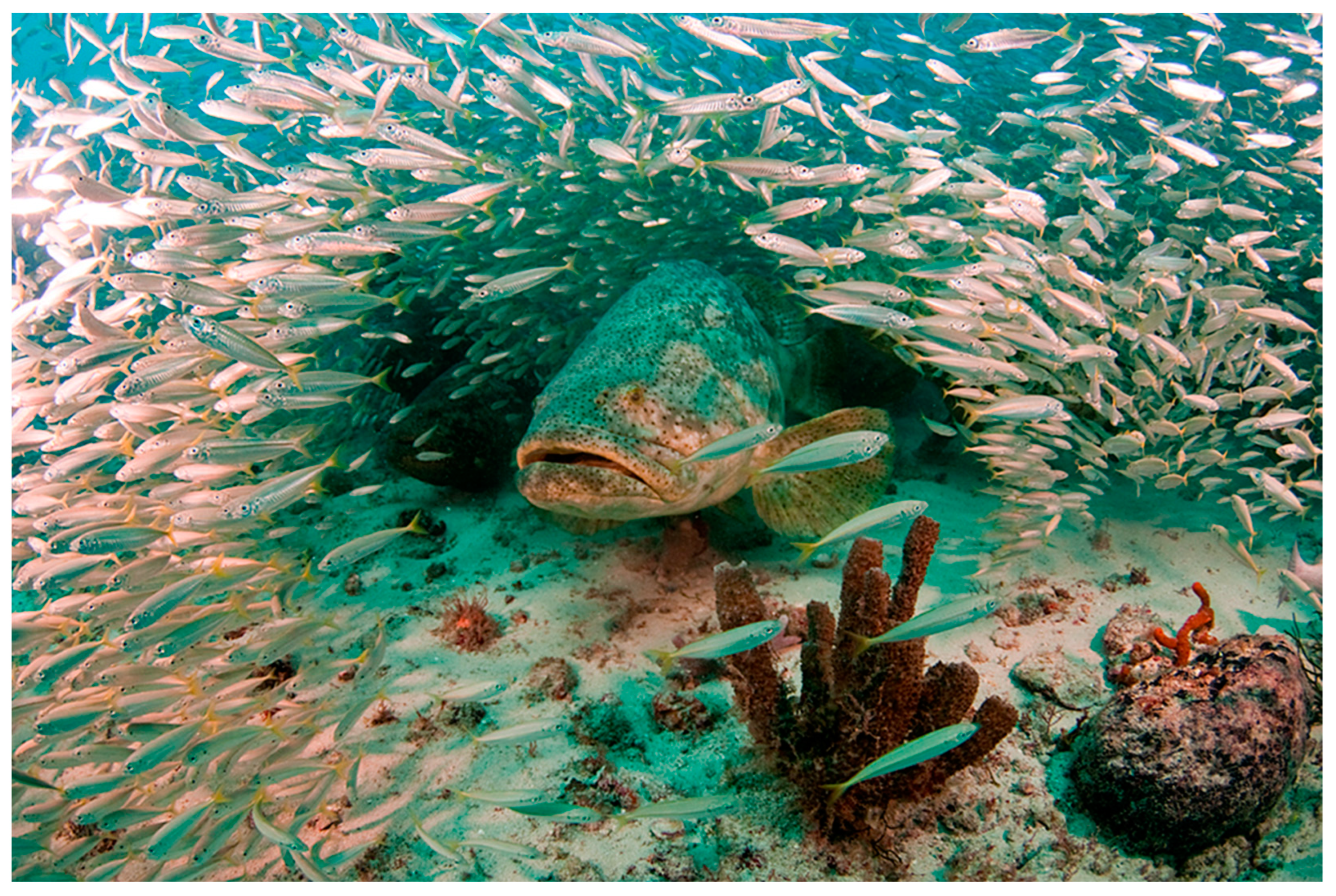
The Florida Fish and Wildlife Conservation Commission, FWC, is currently evaluating analytical approaches that involve non-lethal genetic sampling-and-release as means of abundance estimation for the Atlantic Goliath Grouper (Epinephelus itajara; [7]), hereafter, ‘goliath grouper’ (Figure 1). Goliath grouper is the largest member of the subfamily Epinephelinae in the Atlantic Ocean, reaching lengths of up to 3 m and weighing as much as 400 kg [8]. It is a long-lived, slow-growing marine fish that occupies mangrove and estuarine habitats for up to seven years before relocating as adults to nearshore and offshore reef environments [9]. Reproductive maturity reportedly occurs at ages 6–7 for females and ages 4–6 for males [10]. The oldest known goliath grouper was 37 years old [10] and was collected from waters of the Florida Gulf of Mexico. Adults tend to be solitary and territorial but aggregate to spawn during summer months [11].

As with many large-bodied reef fishes, goliath grouper populations are vulnerable to overfishing owing to relatively slow maturation, spawning aggregation behavior, a limited and increasingly degraded juvenile habitat, and high fishery desirability [12,13]. Relevant reproductive characteristics of this species are summarized in

Table 1. Reproductive life history traits and measures for the modeled population.

Traits and Measures	Atlantic Goliath Grouper	Reference
Age at maturity	$x_{\alpha }$= 6–7 years (f); 4–5 years (m)	[10]
Longevity	$x_{\omega }$= 37–38 years; possibly truncated	[18]
Reproductive lifespan	$\tau$= 30–31 years (f); 32–33 years (m)	${\tau }_y=x_{{\omega }_y}-x_{{\alpha }_y}$
Spawning habitat	Rocky reefs/artificial reefs/wrecks; depths of 15–50 m	[19]
Spawning season	August through mid-October	[9,11]
Spawning mode	Broadcast spawning in small groups or aggregations	[11,20,21,22]
Reproductive strategy	Possibly diandric protogynous	(C. Koenig, pers. comm.)
Mean batch fecundity	~50 × 106	[23]
Maximum body weight	310 kg	[12]
Maximum body length	244 cm	[12]
Female spawning frequency	unknown	--
Spawning site fidelity	84% return at 1-year interval; 78% at 2-year interval	[11]
Pelagic larval duration	30–80 d	[24]
Settlement habitat	Mangrove leaf litter	[9,18]
Juvenile habitat	Mangrove forests bordering rivers and islands	[9]

. The species was once considered to be critically endangered by the International Union for Conservation of Nature, IUCN, and is thought to be overfished throughout most of its range [14,15]. However, populations in coastal waters of the Southeastern United States have shown signs of recovery, in large part owing to an exclusive-economic-zone-wide fishing moratorium instituted in 1990 [16]. As a result, the species was downlisted to vulnerable status by the ICUN [17]. While the apparent improvement in goliath grouper populations is encouraging, more information is needed regarding spawning stock abundance. Preliminary genetic sampling and background modeling is underway by the FWC to evaluate the application of CKMR to spawning stocks along the east and west coasts of Florida.

To support this evaluation, I extended a discrete-time, age-structured, deterministic model [25] with a data-informed prediction of the model’s Poisson scaling factor, $\varphi$, to obtain information on the mean and variance of both annual reproductive success, ARS, and lifetime reproductive success, LRS. Model initialization utilized vital rates and life history measures obtained or synthesized from the most recent Southeast Data, Assessment, and Review (SEDAR) 47 Final Stock Assessment Report [18] and exploratory values of $N_A$. To predict $\varphi$, the model extension relied on a precise empirical genetic estimate of $N_e$ from the Florida Atlantic goliath grouper population. This $N_e$ estimate was based on a single-sample linkage disequilibrium analysis of multilocus genotypes derived from 33 variable microsatellite DNA loci.

Conditions and circumstances that potentially influence population vital rates (e.g., fishing mortality, compensation, and depensation) and other life history variables (e.g., sex reversal, age truncation, and early maturation) warranted attention during modeling. Because of the supposition that age classes are truncated [18], goliath grouper survival rates were modeled herein under the lowest posited scenario for maximum age, $x_{\omega }$. Sex change is a common reproductive strategy among groupers [26] and there is increasing evidence (C. Koenig, pers. comm.) that goliath grouper may share a diandric protogynous strategy with the closely related giant grouper, E. lanceolatus [27]. Therefore, possible impacts of diandric sex change on reproductive success dynamics were quantified under varying female-to-male transition rates and patterns.

The population genetic data used to estimate $N_e$ were also used to infer close-kin relationships directly, adopting a de novo empirical Bayes inference approach. The results for modeled reproductive success metrics were interpreted synoptically and within the context of the inferred close-kin relationships. Both analyses were used to evaluate the conformance of those metrics to CKMR assumptions and other aspects of abundance estimation for goliath grouper. The very low estimated values of $N_e$ for the Florida Atlantic population also motivated a precautionary consideration of prospects for genetic security and reproductive resiliency in the face of erratic environmental conditions and other population stressors.

2. Materials and Methods

2.1. Model Formulation

Parameter notations used for the model are provided in Box 1.

Box 1. Parameter notations used for the hFHM. Accents for these notations are described in the text.

$N_x$	Number of individuals of age $x$ alive at a given time
$N_A$	Number of potential adult breeders in a population
$N_{A+J}$	Total number of individuals (adults and juveniles) in a population
$T$	Length of a generation in years (see definition in text)
$N_e$	Generation effective population size (for age-structured populations)
$N_b$	Effective number of breeders producing a single-year class
${\overline{k}}^{*}$	Mean lifetime reproductive success of breeders during a generation
$V_k^{*}$	Lifetime variance in reproductive success among breeders in a population
$\overline{k}$	Mean reproductive success of breeders in one time period (e.g., annually)
$V_k$	Variance in the number of newborns produced by all breeders in one time period (e.g., annually)
$b_{x,y}$	Mean fecundities at age $x$ and sex $y$; $b_{x,y}$ is scaled to constant $N_{A+J}$, with the quantity becoming ${\dot{b}}_{x,y}$
$B_{x,y}$	Mean number of newborn births produced by breeders of age x and sex y
$s_{x,y}$	Probability of survival from age $x$ to age $x$ + 1 for sex $y$
$l_{x,y}$	Cumulative survival through age $x$ and sex $y$, where $l_1=1$ and $l_{x,y}=l_{x,y-1}{s}_{x,y-1}$ for $x>1$
$x_{\alpha }$	Age at maturity
$x_{\omega }$	Maximum age
${\varphi }_{x,y}$	Poisson scaling parameter for birth rate at age $x$ and sex $y$ in a given time period; ${\varphi }_{x,y}=V_{k,x,y}/B_{x,y}$
$\psi$	Dispersion parameter for annual reproductive success; $\phi =V_k/\overline{k}$
${\psi }^{*}$	Dispersion parameter for lifetime reproductive success; ${\phi }^{*}=V_k^{*}/{\overline{k}}^{*}$

For diploid organisms with overlapping generations, ${\overline{k}}^{*}$ should roughly equate to ${\overline{k}}^{*}\approx 2$ when per capita births equal deaths in the population over the timescale of a few generations. Reproduction is considered to be successful when parents produce offspring that survive to reproductive age [28]. Ignoring second-order terms and assuming equality in male and female dynamics, the generation effective sizes, $N_e$, of such populations can be quantified by Hill’s [29] equation as follows:

$$N_e\approx 2{\overline{k}}^{*}{N}_{\eta }T/\left[V_k^{*}+2\right]$$

(1)

where $N_{\eta }$ is the number of newborn individuals in a given year class $\eta$, $T$ is the length of the generation time, and $V_k^{*}$ is the variance in LRS that applies to the newborn cohorts (new year classes). This formula, although given by Hill in terms of family size variance, also applies as an inbreeding effective size in random mating populations of a constant size [30].

Using the standard discrete-generation formula for inbreeding effective size [31], the effective number of breeders, $N_b$, for a given year class is as follows:

$$N_b=\left[\overline{k}{N}_A-2\right]/\left[\overline{k}-1+V_k/\overline{k}\right]$$

(2)

remembering that $\overline{k}$ and $V_k$ are the mean and variance, respectively, in the number of newborns produced by all potential male and female breeders in one time period (herein, annually) that survive to reproductive age. Separating the variance into male and female components yields the following:

$$N_b=4/\left[\left[V_{k,f}+{\overline{k}}_f \left({\overline{k}}_f-1\right)/{\overline{k}}_f \left({\overline{k}}_f{N}_{A,f}-1\right)\right]+\left[V_{k,m}+{\overline{k}}_m \left({\overline{k}}_m-1\right)/{\overline{k}}_m \left({\overline{k}}_m{N}_{A,m}-1\right)\right]\right]$$

(3)

where $f \mathrm{and} m$ subscripts denote female and male contributions, respectively. As a point of interest, the left and right bracketed terms in the denominator in Equation (3) represent sampling probabilities for shared maternity and paternity, respectively, for any pair of randomly selected offspring in the cohort. Expressions for estimating effective number of breeders can also be derived in terms of the sampling probabilities for HSPs and full sibling pairs, FSPs [5,32].

In a very useful innovation, Waples et al. [25] integrated Hill’s [33] and Crow and Denniston’s [31] statistical formulations with a demographically oriented approach advanced by Felsenstein [34]. Their hybrid Felsenstein–Hill model, $\mathrm{hFHM}$, which adopts properties of the well-known Leslie matrix [35], can be applied to gonochoristic or sex-changing organisms, and does not assume equality in male and female dynamics. Breeders of age $x$ and sex $y$ produce an average of $B_{x,y}$ offspring that survive to age $x+1$ with an annual probability $s_{x.y}$ or perish. Waples et al. [25] defined the age-/sex-specific Poisson scaling factor ${\varphi }_{x,y}$ as the ratio of the variance to the mean reproductive success in one spawning season (i.e., annually) for breeders of a given age and sex (${\varphi }_{x,y}=V_{x,y}/B_{x,y}$). In essence, ${\varphi }_{x,y}$ quantifies the magnitude of ‘within-age’ effects for a given sex. When Poisson expectations for reproductive success of same-age same-sex breeders are random, each age and sex can be viewed as a mini-Wright–Fisher ideal population, such that ${\varphi }_{x,y}\approx 1$ and values of ${\varphi }_{x,y}>1$ represent the degrees to which annual variance in reproductive success is overdispersed relative to respective mean birth rates.

As in Hill’s equation, the hybrid model assumes dynamic stability in age structure and population size over several generation intervals as well as independent probabilities of survival and reproduction [33]. Geographic closure is assumed for population dynamics (i.e., no appreciable effect on birth and death rates owing to immigration or emigration in the modeled demographic unit); see Waples and England [36] and Ryman et al. [37], for additional considerations.

With life table input and an independent estimate of $N_e$, sex-specific measures of the reproductive success metrics ${\overline{k}}^{*}$, $V_k^{*}$, $N_b$, $\overline{k}$, and $V_k$ can be obtained from the hFHM through a novel use of the program AgeNe ([25]; Ecological Archives E092-126-S1). For a given life table, AgeNe evaluates the above parameters using a three-step sum of squares approach. Initial model conditions are set with requisite user input for age-specific (proportional) sex ratio, $S{R}_{x,y}$, and values of $x_{{\omega }_y}$, $N_1$, and ${\varphi }_{x,y}$ (here, the demographic clock is set by defining $N_h$ as the number of fertilized gametes (hatched eggs) that enter the system as a discrete annual cohort and $N_1$ as the number of ‘newborn’ offspring in their first year of life, which, in fishery terms, would be analogous to the number of young-of-the-year fish (traditionally, fishery biologists define young-of-the-year cohorts as age-0 or age-0+; linking ages thus represents a practicality, as AgeNe does not accept sub-one values as input for age)). For the parameter $N_{\eta }$, it has been pointed out [6,38] that any year class from age-one, $x_1$, to age-at-maturity, $x_{{\alpha }_y}$, can be adopted to evaluate the sensitivities of model parameters to changes in $N_e/N_A$ and $N_b/N_A$. Likewise, the model calibrated value of ${\varphi }_{x,y}$ is not affected by this cohort choice. Thus, for convenience, I evaluated parameter values of interest at $N_1$.

Values of $N_1$ will usually be unknown, as is the case for the studied population, but can be estimated from a partial life table ($s_{x,y}, x_{\alpha }{}_y, x_{\omega }{}_y$, and $S{R}_{x,y}$) when either an empirical estimate of $N_A$ is available or a plausible exploratory range of $N_A$ is specified. Investigators might have empirical knowledge of that range from fishery acoustic surveys [39], physical tagging [40], or GCMR/CKMR [2,3]. Lacking such information for goliath grouper, values of $N_1$ were tallied in a partial life table given initial exploratory values for $N_A$ (see Supplementary File S1) and used as input for various model constructions.

For simplicity, I assumed that the scaling factor ${\varphi }_{x,y}$ was constant over all ages and between sexes; subscripts in that case were dropped. Not surprisingly, true values of $\varphi$, while critical to the modeling and investigation of reproductive success dynamics, are rarely known for iteroparous marine fish populations. Therefore, I developed a method to predict $\varphi$ through an extension of the hFHM and by relying on a generally available data source—population genotype data. To distinguish it from the standard model, the predictive model is denoted as scFHM. With functionality rooted in the hFHM, the scFHM has flexibility to accommodate constant or variable values for age- or sex-specific survival, age- or sex-specific fecundity, and age-specific sex ratio. During prediction, empirical estimates of $N_e$ or $N_b$, when available, can be used as independent variables to solve model-generated functions for $\overrightarrow{\varphi }$. For this purpose, a precise empirical estimate of $N_e$ was obtained from population genotypes, as described below.

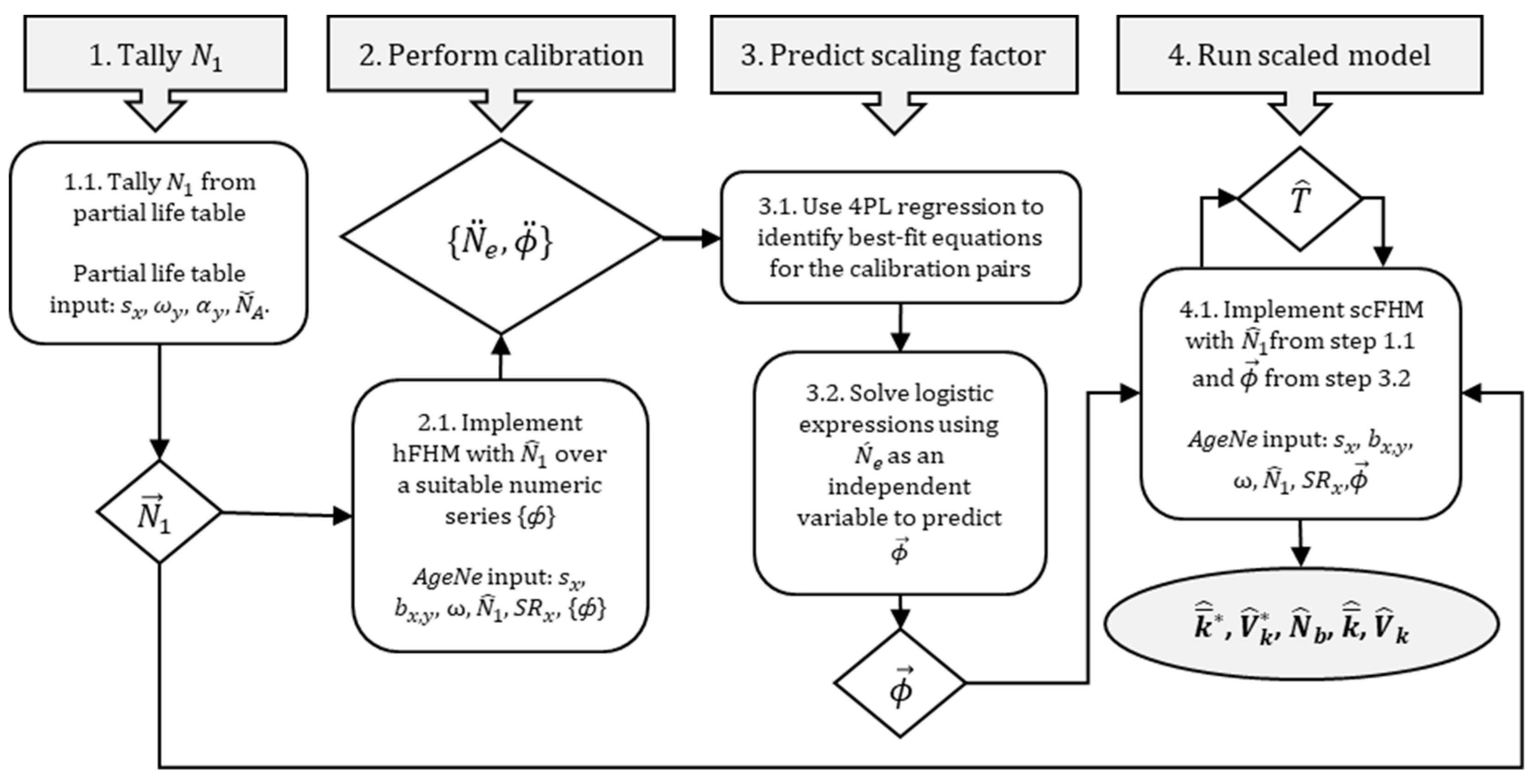
For the scFHM, tallied values of ${\overrightarrow{N}}_1$ along with requisite life table information were first used to initialize the hFHM. A series of calibration points were evaluated in separate model runs for a given set of conditions to generate paired data—i.e., {${\ddot{N}}_e$ at $\ddot{\varphi }$}—for use in prediction. Best-fit predictive functions were obtained via logistic regression. For curve fitting, a minimization process was used to identify a single curve that best described the data—i.e., parameter values of the curve were adjusted until the lowest possible residual sum of square error was observed. Goodness-of-fit for linear regressions was assessed via F-statistics and R² values. Predicted values, $\overrightarrow{\varphi }$, from resultant functions were then carried back into the hFHM to scale final estimates of ${\widehat{V}}_k$, $\widehat{\overline{k}}$, ${\widehat{N}}_B$, and ${\widehat{V}}_k^{*}$. It is noted that, when empirical estimates of ${\acute{N}}_B$ are available instead of ${\acute{N}}_e$, {${\ddot{N}}_B$ at $\ddot{\varphi }$} can be calibrated instead to infer ${\widehat{V}}_k$, $\widehat{\overline{k}}$, ${\widehat{N}}_e$, and ${\widehat{V}}_k^{*}$. The entire process is summarized in Figure 2.

2.2. Tissue Collections

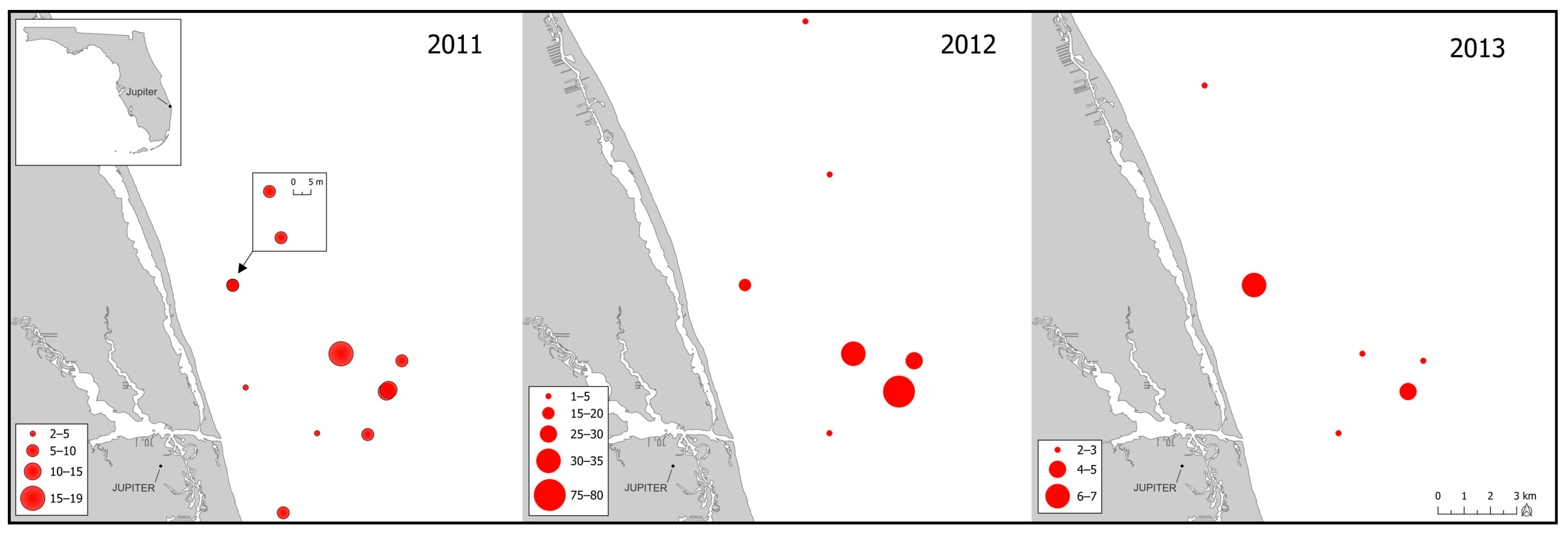
Study tissues from Florida Atlantic specimens were procured from colleagues at the Florida State University, FSU, Coastal Marine Laboratory. Tissue collections occurred during 2011 to 2013 within Florida Atlantic coastal waters (Figure 3) and consisted of fin clips and fin rays. Tissues were stored in 95% ethanol until processing. Fish were aged by FSU biologists using sampled fin-rays and methods described in Murie et al. [41]. Fish sizes, ages, collection dates, and GPS collection coordinates were available for most specimens; primary collection data appear in Table S2 of Supplementary File S2.

2.3. Genealogical Inference

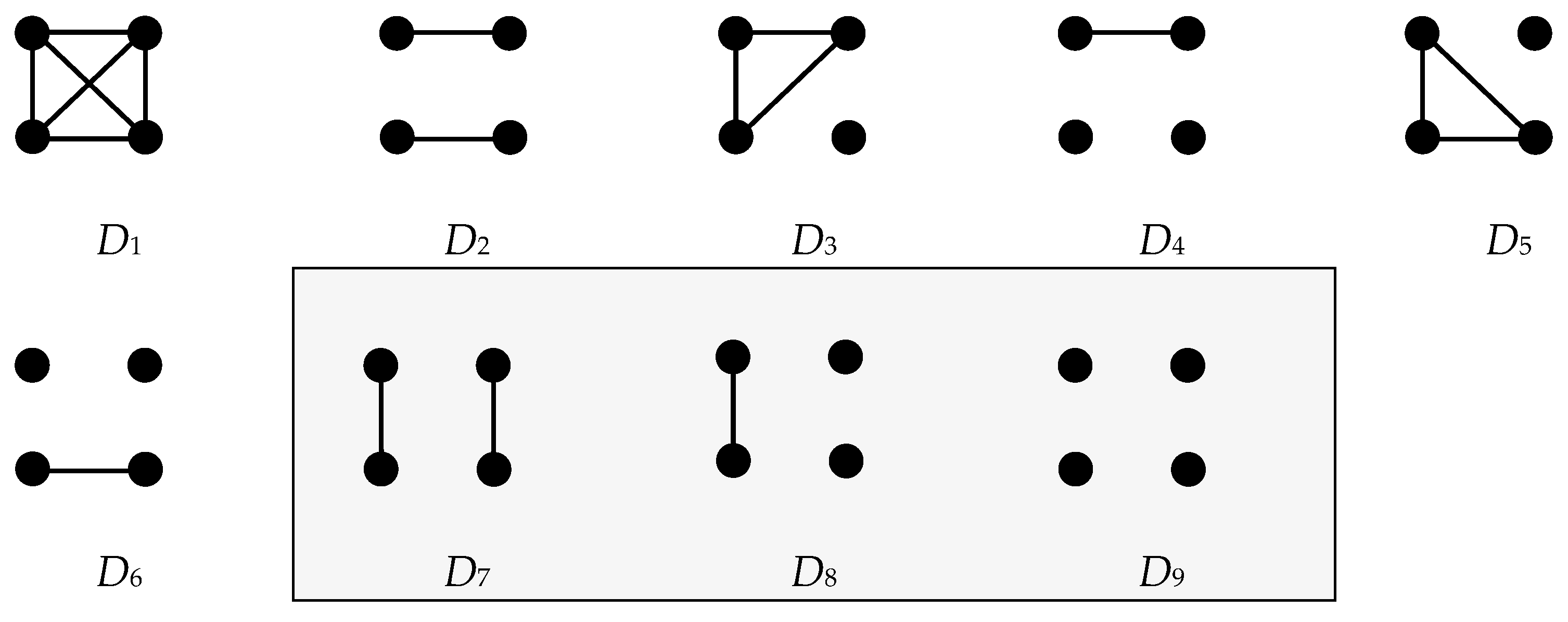
Population genotype data were based on fragment-size analyses of 36 microsatellite DNA markers. Molecular procedures, including marker description, laboratory quality assurance, and quality control protocols, and standard diversity analyses are described in Supplementary File S2. Because classification of close kin involved multiple paired comparisons of categorical relationships, $\mathcal{R}$, from a natural population of unknown abundance and for which sampling probabilities (i.e., priors) of the categorical relationships of interest were unknown, I developed a de novo empirical Bayes inference model for the task. The flexible approach allowed paired evaluation of all genotypes over a heuristically valid ensemble of $𝓇$ = 9 plausible categorical relationships (Appendix A). Given the sufficiency in cumulative likelihoods from the locus number and allele polymorphism (Appendix B), the sampling priors of these nine relationships can be reasonably approximated from the population genotype data via an optimization algorithm and employed as mixing weights to greatly improve the classification accuracy (Appendix C). With a Bayes maximum a posteriori (MAP) classifier (Appendix D) and a base model calibrated with reasonably accurate mixing weights, marginal posterior expectations yield reliable predictive distributions and belief measures.

It must be noted that genotypes from independently segregating genetic loci cannot distinguish half-sibling relationships from those of avuncular and grandparent–grandchild; therefore, the acronym is hereafter denoted as HSP⁺.

2.4. Empirical Estimation of Effective Population Size

The single-sample linkage disequilibrium, LD, analysis option in NeEstimator V2.1 [42] was used to generate raw estimates of generation effective population size, ${\tilde{N}}_e$, for the sampled population. Estimates were formulated from the squared correlation of alleles at independently segregating gene loci [43,44]. LD analysis is based on the principle that, in closed finite populations in approximate drift–mutation–recombination equilibrium, associations between alleles among selectively neutral gene loci are a function of the generation of an effective population size. For this analysis, the moment-based genetic index is Equation (4) [43,44]:

$$E\left(r^2\right)\approx \frac{1}{3N_e}+\frac{1}{n_g}$$

(4)

Rewriting Equation (4) and including the sampling bias adjustment of Waples [45], ${\tilde{N}}_e$ was obtained in NeEstimator from expected levels of allele association across loci, $r^2$, as follows:

$${\tilde{N}}_e=1/\left(3\left(r^2-1/n_g\right)\right)$$

(5)

Because $n_g$ varies among loci, its harmonic mean was used in Equation (5). Missing data were tabulated for each run and potential effects of low-frequency alleles on estimates were mitigated by adopting a nominal type I error rate ($P_{crit}$) value of 0.01 [44]. Parametric 95% and pseudo-jackknife confidence intervals [46] were recorded for all runs. Finally, raw estimates from NeEstimator were adjusted in silico using correction factors for physical linkage among loci [47] and mixed-age sampling [48], as described in Supplementary File S2, yielding a bias-adjusted estimate of ${\acute{N}}_e$ for modeling and conservation assessment.

Waples [49] described a systemic tendency for ${\tilde{N}}_e$ to be imprecise for the LD procedure when there is either insufficient sampling of individuals, loci, or both. Owing to stochastic effects in genetic drift and sampling error, mean values of the moment-based index approach theoretical expectations for large values of $n_g$ and $\hat{\mathcal{K}}$, where $\hat{\mathcal{K}}$ is the number of pairwise comparisons among $𝓀$ independent alleles. Statistical precision for the goliath grouper estimate was evaluated by examining the coefficient of variation, CV, on ${\acute{N}}_e$ as follows:

$$C{V}_{{\acute{N}}_e}=\sqrt{2/\widehat{\mathcal{K}}}\left[1+\frac{3N_e}{n_g}\right].$$

(6)

Because $N_e$ in the numerator of the above expression denotes the true value, I conservatively used the upper confidence interval ($CI$) of the ${\acute{N}}_e$ estimate in its place. The harmonic mean value of $n_g$ was also used for the calculation, and $\widehat{\mathcal{K}}$ was adjusted for missing data.

2.5. Life Table Synthesis

Data used to develop $s_{x,y}$ were extracted from the SEDAR 47 Final Stock Assessment Report [18]. The maximum age modeled here was $x_{\omega }$ = 37 years. Male and female Von Bertalanffy growth function parameters were $L_{\infty }$ = 2221 mm total length, $K$ = 0.0937 year⁻¹, and $x_0$ = −0.6842 year. Natural mortality rates, $M_x$, were estimated using the Hoenig_nls method [50], as described in the SEDAR 47 report, and $s_x=e^{-(M_x)}$. Whereas Bullock and Smith [23] estimated batch fecundity for two goliath grouper females to be 38,922,168 ± 1,518,283 and 56,599,306 ± 1,866,130 oocytes, robust age-specific estimates are unavailable. Thus, for fecundity estimation, the gonad weight-at-total-length relationship was established as $G{W}_L=a+bL$, where $a$ = −36132.7 and $b$ = 24.5 [18]. Relative fecundity, $b_{rel}$, which is the mean number of eggs per gram of fish weight, was taken as 21,312 eggs/g [18]. Females were assumed to reach maturity at age 6, and female fecundity-at-age, $b_{x,f}$, was estimated to be $b_{x,f}={\rho }_x\left(a+bL\right)b_{rel}$, where ${\rho }_{x,f}$ = proportion mature at age $x$/100. Owing to the absence of data for male fecundity, female values were adopted for males aged ≥6 years. For males aged 4 and 5 years, the approximation $b_{x,m}\approx {\rho }_{x,m}$ was used.

The quantity $b_{x,y}$ was scaled to constant $N_{A+J}$ (for which ${\overline{k}}^{*}=2$) using cumulative survival, $l_{x,y}$, through age $x$ and sex $y$, where $l_1$ = 1 and $l_{x,y}=l_{x-1,y}{s}_{x-1,y}$ for $x>1$ [25], with the scaled quantity denoted as ${\dot{b}}_{x.y}$. Finally, $B_{x,y}$, which is the estimated mean number of newborn births produced by all breeders of age x and sex y, was calculated as $B_{x,y}={\dot{b}}_{x.y}{N}_{x,y}$. The effects of sex change were modeled in two ways. First, a fixed female-to-male ratio, ${\overleftrightarrow{SR}}_x$, of 1:1 was adopted for ages one to four and a simple linear function for female-to-male sex reversal was applied to the remaining age classes, such that $S{R}_{x,f}=0.0061x+0.5242$ for $x\ge 5 \mathrm{years}$. Alternatively, a logistic function $S{R}_{x,f}=0.754+(\left(0.503-0.754\right)/\left(1+{\left(x/8.840\right)}^{4.734}\right)$ for $x\ge 5 \mathrm{years}$ was surveyed to generate female age-specific sex ratios. The s-shape of the logistic function mimics the case where younger adult males transition at a greater rate than older males. For both functions, $S{R}_{x,m}=1-S{R}_{x,f}$.

For goliath grouper, empirical age-composition data were not sufficiently developed for a direct estimate of $T$ [18], but the generation length has been previously reported to be $T\approx x_{\alpha }+((x_{\omega }-x_{\alpha })/2\approx$ 21.5 years, where $x_{\alpha }\approx$ 6 years and $x_{\omega }\approx$ 37 years. Here, I used a sex-specific measure of $T$ that better accommodates the dynamic factors modeled, reflecting the average age of the parents of all newborn individuals in the modeled population. Estimates of $T_y$ were computed during the course of hFHM runs via the life table equation:

$$T_y={{\displaystyle \sum }}_{x_{{\alpha }_y}}^{x_{{\omega }_y}}\left[x{B}_{x,y}/N_1\right]$$

(7)

2.6. scFHM Runs

For base-model calibration (predictive scaling), exploratory values of ${\check{N}}_A$ = {10,000, 35,000} were combined with model-dependent input values of ${\check{s}}_x$, ${\check{x}}_{\alpha ,y}$, and ${\check{x}}_{\omega ,y}$ to determine ${\overrightarrow{N}}_1$. The above ${\check{N}}_A$ values were spatially explicit, intended to encompass adult goliath grouper residents of Florida Atlantic coastal waters. The calibration set used for predicting the Poisson scaling factor was $\check{\varphi }$ = {1, 25, 50, 150, 300, 750, 1500, 3000, 7500, 11,500, 15,000, 30,000, 75,000}. Predictions of $\overrightarrow{\varphi }$ were performed using point estimates and upper and lower $CI$s of ${\acute{N}}_e$.

In total, three biologically varying model constructions comprising six scFHM runs (78 hFHM runs) were implemented for the predictive phase (

Table 2. Model construction.

Model	Reproduction	Sex Ratio	${\mathit{N}}_{\mathit{A}}$	${\mathit{N}}_1$
M1A	gonochoristic	1:1	10,000 (fixed)	81,575 (tallied)
M1B	gonochoristic	1:1	35,000 (fixed)	285,526 (tallied)
M2A	diandric	linear increase in $S{R}_{x,m}$ with age	35,000 (fixed)	284,300 (tallied)
M3A	diandric	logistic increase in $S{R}_{x,m}$ with age	35,000 (fixed)	281,930 (tallied)
M2B	diandric	linear increase in $S{R}_{x,m}$ with age	35,150 (resultant)	285,526 (fixed)
M3B	diandric	logistic increase in $S{R}_{x,m}$ with age	35,446 (resultant)	285,526 (fixed)

). For the base model, a gonochoristic reproductive strategy and a 1:1 sex ratio was assumed (M1). This model was then modified to accommodate the first diandric protogynous scenario (M2), incorporating the linear pattern of $S{R}_{x,y}$. Finally, the base model was modified to accommodate the second diandric protogynous scenario (M3), incorporating the logistic pattern of $S{R}_{x,y}$. Following the prediction of $\overrightarrow{\varphi }$, 18 scFHM runs were implemented to establish levels of $\psi$, ${\psi }^{*},$ and related parameters for the population. Each of these runs were scaled with the predicted values of $\overrightarrow{\varphi }$ for point estimates and upper and lower $CI$s of ${\acute{N}}_e$.

3. Results

The total number of genotypes resolved for this Florida Atlantic study population was $n_g$ = 300. Standard measures of genetic diversity are reported in Supplementary File S2. In total, $n_D$ = 45,451 pairwise relationships were classified (including two intentionally replicated genotypes), a value that also represents the total probability mass of the empirical sampling probability distribution for $𝓇$. The optimized ${\mathbb{I}}_{\mathcal{R}}$ was {IDP, 3.00; POP, 2.66; FSP, 33.68; HSP⁺, 88.39; FCP, 25.56; HFCP, 27.16; SCP, 46.84; HSCP, 373.44; URP, 44,850.27}, which represents the expected number of each categorical relationship pair given the data. Among those classified, 68 pairs of interest satisfied MAP₅₀ assignment criteria (3 IDPs, 3 POPs, 35 FSPs, and 27 HSP⁺s). A parent–offspring triad consisting of two full siblings and a parent was inferred. Eight multiple-sibling families and an additional POP were inferred. The largest multiple-sibling pedigree consisted of six individuals that formed three FSP and six HSP⁺ relationships. Another 28 single-sibling families were credibly inferred, consisting of 15 FSPs and 13 HSP⁺s. Posterior probabilities of several additional pairs fell short of the MAP₅₀ criterion, but their relationships were indicated by other robust familial assignments.

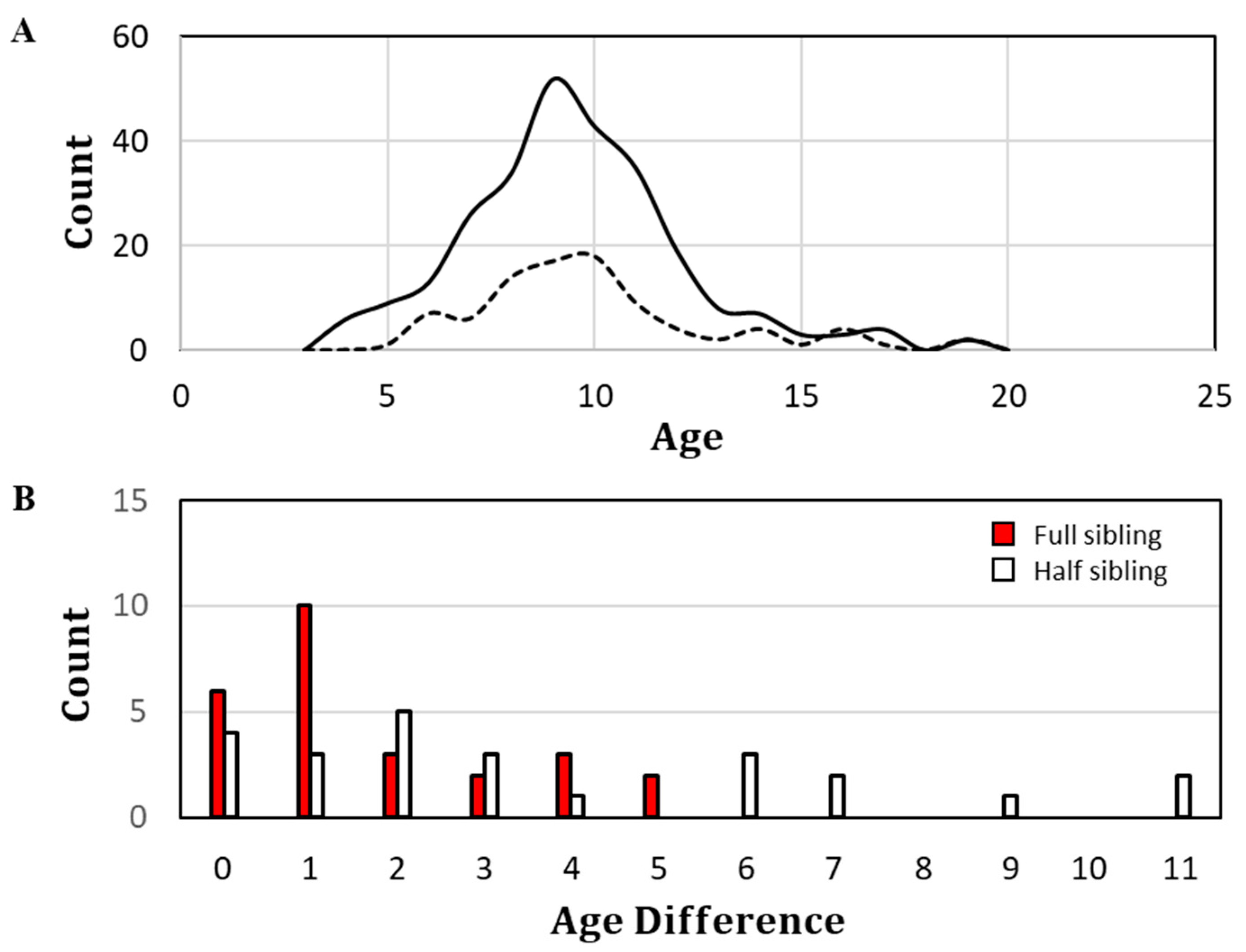
Fin-ray-based ages were assigned for 264 of the 302 specimens. The age compositions of all sampled specimens and members of classified close-kin pairs are depicted in Figure 4A. Most specimens, including those inferred to have paired familial relationships, were between the presumptive ages of 8 and 11 years at the time of their sampling. The minimum observed age was 4 years and the maximum observed age was 19 years. Age differentials between close-kin pairs appear in Figure 4B. FSPs differed in age by as much as 5 years, with the highest percentage (10 of 26) differing by only 1 year. HSP⁺s differed by as much as 11 years, with most differing by 2 years.

3.1. Effective Population Size Estimate

One genotype from each classified IDP was culled from the dataset prior to the estimation of $N_e$, yielding $n_g$ = 299 for this analysis; the harmonic mean sample size was $n_g$ = 289.1. Discounting monomorphic loci, there were 222 single-locus genotypes with missing data out of the (299 × 33) 9867 scored, yielding an overall genotyping efficiency of 98%. Accounting for missing data, the number of possible pairwise comparisons between $𝓀$ independent alleles was $\widehat{\mathcal{K}}$= 43,456. At $P_{crit}$= 0.01, a raw estimate of ${\tilde{N}}_e$ = 402.5 was observed, with $CI$ = 359.3 to 455.2. Upon bias adjustment for mixed-age sampling and physical linkage, ${\acute{N}}_e$ = 658.8 ($CI$ = 588.1 to 745.0). The estimated $C{V}_{{\acute{N}}_e}$ was 0.059, which was very low primarily owing to the large $\widehat{\mathcal{K}}$.

3.2. Demographic Results

Life tables for all calibration models are provided in Supplementary File S3. Base model tallied values of ${\overrightarrow{N}}_1$ were 81,575 and 285,526 for ${\check{N}}_A$ values of 10,000 and 35,000, respectively. However, when ${\check{N}}_A$ was fixed at 35,000 during sex-reversal modeling, tallied values of ${\overrightarrow{N}}_1$ were 284,300 and 281,930 for M2A and M3A, respectively. Sex-specific population abundances for $N_{A+J}$ and $N_A$ are reported in

Table 3. Sex-specific and overall generation lengths and population abundances. Bold type denotes model input. Shaded area highlights differences between male and female abundances.

Model	M1A	M1B	M2A	M2B	M3A	M3B
${\stackrel{\mathbf{ˇ}}{\mathit{N}}}_{\mathit{A}}$	10,000	35,000	35,150	35,000	35,446	35,000
${\overrightarrow{\mathit{N}}}_{\mathbf{1}}$	81,575	285,526	285,526	284,300	285,526	281,930
$\widehat{T}$	20.99	20.99	20.90	20.90	20.92	20.92
${\widehat{T}}_f$	21.10	21.10	20.49	20.49	20.79	20.79
${\widehat{T}}_m$	20.89	20.89	21.31	21.31	21.05	21.05
$N_{A+J,m}$	60,737	212,591	214,147	212,928	218,335	215,585
$N_{A+J,f}$	60,737	212,591	211,033	210,429	206,845	204,242
$N_{A+J}$	121,475	425,182	425,182	423,357	425,180	419,827
$N_{A,m}$	6220	21,771	23,175	23,078	26,412	26,079
$N_{A,f}$	3780	13,229	11,975	11,922	9003	8921

. Estimates of $\widehat{T}$ are independent of modeled values of ${\overrightarrow{N}}_1$. For the base model (M1), $\widehat{T}$ was estimated to be 20.99 years (Table 3). Whereas this model estimator was based on both fecundity and mortality, the result was comparable to the coarsely approximated value of 21.5 years based solely on $x_{\omega }$ and $x_{\alpha }$. When M2 and M3 sex-reversal dynamics were incorporated, overall estimates of generation length decreased very slightly compared with those of M1. Expectedly, male $T$ values were slightly higher than those of females (Table 3).

The linear transition formula in M2 (Figure 5A) led to a relatively modest shift from the initial female-to-male ${\overleftrightarrow{SR}}_{x=1 \mathrm{to} \alpha }$ of $\approx$1:1 to that of ${\overleftrightarrow{SR}}_{x=38}\approx$1:2.25. With a fixed value of ${\overrightarrow{N}}_1$, this formula resulted in slightly more male breeders in the population and an overall adult female-to-male ratio of ${\overleftrightarrow{SR}}_{x=\alpha \mathrm{to} \omega }\approx$1:1.94. Likewise, minimal change was observed when the value of ${\check{N}}_A$ was fixed; ${\overleftrightarrow{SR}}_{x=\alpha \mathrm{to} \omega }\approx$1:1.94. The logistic transition formula in M3 (Figure 5B) led to a somewhat higher shift; ${\overleftrightarrow{SR}}_{x=38}\approx$ 1:3.16. Overall adult ratios for M3 were ${\overleftrightarrow{SR}}_{x=\alpha \mathrm{to} \omega }\approx$1:2.93, respectively, whether ${\overrightarrow{N}}_1$ or ${\check{N}}_A$ were fixed.

3.3. Reproductive Success Metrics

All best-fit predictive curves from the logistic regression were recovered with high precision ($R^2$ > 0.999999999999). Robust predictive behavior was not unexpected given the underlying deterministic process model. Thus, $\overrightarrow{\varphi }$ can be extrapolated in predictive plots with sufficient accuracy (Figure 6) during workflow step 3.2 (Figure 2).

In scaled-model runs (step 4.1 of the scFHM workflow; Figure 2), all three model constructions were first evaluated with common values of ${\overrightarrow{N}}_1$ = {81,575; 285,526} and model-specific $\overrightarrow{\varphi }$ values. They were then evaluated with common values of ${\check{N}}_A$ = {35,000} and model-specific $\overrightarrow{\varphi }$ values (see Table 2). Overall, levels of $\psi$ and ${\psi }^{*}$ were very high and positively related to modeled values of ${\overrightarrow{N}}_1$ (

Table 4. scFHM results for each model construction.

	Model	M1A	M1B	M2A	M2B	M3A	M3B
Input	${\check{N}}_A$	10,000	35,000	35,151	35,000	35,446	35,000
	${\overrightarrow{N}}_1$	81,575	285,526	285,526	284,300	285,526	281,930
	${\acute{N}}_e$	658.77	658.77	658.77	658.77	658.77	658.77
	$\overrightarrow{\varphi }$	3898.64	16,896.17	16,781.89	16,703.58	16,454.12	16,226.14
ARS	${\widehat{V}}_k$	5354	22,811	22,661	22,556	22,252	21,946
	${\widehat{V}}_{k,f}$	5356	22,812	22,852	22,746	22,947	22,632
	${\widehat{V}}_{k,m}$	5352	22,809	22,473	22,369	21,595	21,297
	$\widehat{\overline{k}}$	1.34	1.34	1.34	1.34	1.34	1.34
	${\widehat{\overline{k}}}_f$	1.34	1.34	1.35	1.35	1.38	1.38
	${\widehat{\overline{k}}}_m$	1.34	1.34	1.33	1.33	1.31	1.31
	${\widehat{N}}_B$	40.9	33.6	33.8	33.9	34.5	34.5
	${\widehat{N}}_{B,f}$	20.5	16.8	16.9	16.9	17.2	17.2
	${\widehat{N}}_{B,m}$	20.5	16.8	16.9	16.9	17.3	17.3
	$\psi$	2677	16,985	16,874	16,795	16,569	16,341
	${\psi }_f$	2678	16,986	16,890	16,811	16,628	16,400
	${\psi }_m$	2676	16,984	16,859	16,781	16,510	16,282
LRS	$V_k^{*}$	10,395	36,390	36,233	36,077	36,267	35,811
	${\psi }^{*}$	5198	18,195	18,117	18,038	18,134	17,906

). Based on the point estimate for ${\acute{N}}_e$, inferred values of ${\widehat{V}}_k$ and ${\widehat{V}}_k^{*}$ for goliath grouper were extremely high, ranging from 5354 to 22,811 for ${\widehat{V}}_k$ and from 10,395 to 36,390 for ${\widehat{V}}_k^{*}$. Values of ${\widehat{N}}_b$ were very low, ranging from 17.2 to 40.9. The incorporation of sex reversal had a minimal reductive effect on those variance estimates, by way of a reductive effect on $\varphi$, and a minimal but enlarging effect on the effective number of breeders. The effects were greater in M3 than in M2 and greatest in M3B. Calibration data for $\widehat{\varphi }$ predictions; parameter values for logistic equations; and final scFHM estimates of ${\widehat{\overline{k}}}^{*}$, ${\widehat{V}}_k^{*}$, ${\widehat{N}}_b$, $\widehat{\overline{k}}$, and ${\widehat{V}}_k$ based on upper and lower $CI$ values of ${\acute{N}}_e$ are provided in Supplementary File S3.

4. Discussion

Here, a scaled version of Waples et al.’s [25] hybrid Felsenstein–Hill model was used to infer sex-specific estimates of reproductive success metrics that, within the context of relevant demographic rates and measures, were consistent with an independent estimate of $N_e$. To the best of my knowledge, the empirical $N_e$ estimate for this Florida Atlantic population represents a first documentation of effective population size for goliath grouper. The very low observed value of $N_e$ was associated with highly overdispersed variance in lifetime and annual reproductive success. Indeed, the modeled level of ${\psi }^{*}$ exceeded by two orders of magnitude those inferred for red drum and southern bluefin tuna. The model results were only minorly impacted at both annual and lifetime scales by the inclusion of sex reversal dynamics, as will be reviewed in the following section.

The interpretation of results for this particular application of the hFHM relies on a host of factors, but a major limiting factor appears to be the rigorous individual and allelic sampling requirements for empirical $N_e$ estimates, which have rarely been met in past studies of large marine populations (see also [49]). For goliath grouper, a large number of moderately polymorphic loci were genotyped, permitting more than 43,000 paired comparisons of $𝓀$ independent alleles. The number of the individuals surveyed was of the same magnitude as the $N_e$ estimate itself, which satisfied a general guideline from Waples [49]. As a result, the coefficient of variation for the $N_e$ estimate was very low, suggestive of good precision. Empirical precision was also reflected in the upper and lower $CI$s, which were close in value to the point estimate. Thus, it appears the estimate for the time period to which it applies was sufficiently precise so as to robustly support the study findings and conclusions. Other empirical approaches exist for estimating $N_e$ (reviewed in [51]) that carry conditions and assumptions that require careful consideration. It should be noted that empirical estimates of $N_B$, when available, can also be used to predict $\varphi$.

The choices of $N_A$ explored in the model may seem low at a glance, but for two aspects. First, the empirical estimate of $N_e$ used to scale the model is a generational estimate that applies to the reproductive successes of the parents of study specimens, which were alive and breeding back when adult abundances in the Florida Atlantic region were considerably lower. This aspect will be discussed further in Section 4.2 in regard to kinship structure. Second, when $N_e$ is treated as a known value in the scFHM workflow, the magnitudes of $\varphi$ and $V_k$ scale with the tallied value of $N_{\eta }$, which increases when larger values of $N_A$ are modeled. If the exploratory values of $N_A$ were indeed too small, it would only serve to heighten ramifications for CKMR associated with the very high levels of overdispersion.

A new genetic survey by FWC scientists of sampled-and-released adult and juvenile goliath grouper is currently underway in both the Florida Atlantic and Florida Gulf of Mexico, starting in 2019. Those data, when they become available for analysis, will provide an opportunity to determine whether reproductive success dynamics have improved over the interval period.

4.1. Influences of Fishing Pressure and Sex Reversal

The absence of information on possible compensatory or depensatory responses precluded a direct examination of fishing pressure effects, alone and in conjunction with sex reversal. Nonetheless, general impacts of harvest on reproductive success dynamics are predictable. Even when compensatory responses maintain $N_{\eta }$, harvest can lead to decreased generation lengths through the loss of older individuals [52,53] and perhaps earlier maturation [54]. $N_e$ would be expected to decrease with reductions in $T$ caused by age truncation and be exacerbated further by earlier maturation [38,55]. In populations lacking a compensatory reserve [56] and/or subject to depensatory responses, fishing mortality could simultaneously reduce $V_k^{*}$, which could offset changes to $N_e$ caused by reductions in $T$, so the effects must be modeled jointly.

In diandric protogynous populations, some members are born as primary males while others transition from females to secondary males during adulthood, presumably in response to social, behavioral, or environmental cues [57]. Under intense fishing pressure, sex reversal rates can also be a product of compensatory density dependence. Given these circumstances, male abundance, fertilization success, and stock productivity can all be affected by the spatio–temporal dynamics of asynchronous transitioning. Certain forms of selective harvest can skew population sex ratios in a manner that reduces reproductive potential [58,59,60]. For example, in gag (Mycteroperca microlepis), sex change is believed to occur mostly (but not entirely) within the pre-spawning habitat. This habitat seems to represent a critical source of male recruitment to the spawning grounds, where many males are believed to become year-round residents. High fishing pressure in pre-spawning habitat areas, while at the same time also causing age truncation, appears to have played a role in the current female-to-male $\overleftrightarrow{SR}$ in the eastern Gulf of Mexico, which has been estimated to be ~49:1 [61]. Gag likely represents a somewhat worst-case circumstance within the grouper–snapper complex of Serranid fishes [12].

Neither Bullock et al. [10] nor Koenig and Coleman [11] found evidence that the adult $\overleftrightarrow{SR}$ of goliath grouper differs significantly from 1:1. The resultant sex ratios from M2A/B and M3A/B were thus not consistent with the above field observations, as they resulted in ~1:2 and ~1:3 adult female-to-male ratios, respectively. More research data on the true sex reversal dynamics of goliath grouper are needed for a species-specific assessment. In both models of sex reversal investigated here, increases in $T$ for males were offset by decreases for females such that the overall estimated generation lengths did not differ meaningfully from that of the base model (Table 3). M2 and M3 sex reversal dynamics resulted in only very small decreases in $V_k$ in comparison with M1B, with the more extreme (logistic) transition pattern (M3) showing the greatest reduction. These decreases were associated with reduced values of ${\overrightarrow{N}}_1$ (Table 4). Consistent with the variance decreases, values of $N_B$ showed corresponding but slight increases in M2 and M3.

Under fully identical male and female demographic rates and conditions ($s_{x,m}=s_{x,f},$ $b_{x,m}=b_{x,f}, x_{{\alpha }_m}=x_{{\alpha }_f}$, and $x_{{\omega }_m}=x_{{\omega }_f}$), it would be expected that sex reversal would have minimal, if any, enlarging effects on $V_k$ and $V_k^{*}$, and thus very slight reductive effects on $N_B$ and $N_e$. However, modeled maturity schedules and age-specific fecundities were not the same for goliath grouper males and females. Because $s_{x,m}=s_{x,f}$ and $x_{{\omega }_m}=x_{{\omega }_f}$ in all goliath grouper models, the minor differences observed between M1B and M2/3 and their directional effects must have been associated with earlier maturation in males. For the most part, sex-specific changes in reproductive success metrics of goliath grouper caused by sex reversal were offsetting, such that overall values (male + female) of $\psi$ were not greatly affected. These results suggested that sex reversal itself will not have a significant impact on $V_k$, $V_k^{*}$, $N_B$, or $N_e$ for goliath grouper unless it is accompanied by aggravating factors that significantly and disproportionately alter fecundity and/or mortality in a sex-specific manner, such as the size-selective fishing previously discussed for gag. The offsetting tendencies and sensitivities to aggravating factors are expected to be similar for protandrous hermaphroditic fishes (e.g., common snook, Centropomus undecimalis [62]).

4.2. Kinship Distribution and Spatial Dynamics of Close Kin

It would be a reasonable a priori expectation that the prevalence of full siblings (and other ‘full’ relations) would be quite low in natural populations of iteroparous species with indeterminate fecundity, especially broadcast-spawning species whose members aggregate over protracted spawning seasons and repeat this over decadal time scales. Therefore, some may find it surprising that so much of the optimized sampling probability mass was assigned to full-sibling relationships (nearly one-third of that assigned to presumptive half-siblings). Whereas other grouper species (e.g., gag and red grouper, Epinephelus morio) are known to spawn in pairs, it has been posited based on male gonad size and sperm quantity that goliath grouper spawn in multi-male groups [22]. That may indeed be the evolved strategy, applicable when the temporospatial availability of breeders permits it. However, the only documented direct observation of goliath grouper spawning involved one female and only two males [22]. If it was true that females were accompanied more frequently than presumed by only a few males during their “spawning rushes” to the surface, it would not be unusual to have encountered littermates among offspring within year classes. Still, given the lengthy reproductive lifespan of adults, a somewhat high prevalence of cross-year-class FSPs is harder to reconcile biologically without evoking circumstances of frequent paired mating, very high spawning site fidelity, or other special circumstances.

At the times and places that sampling occurred for this study (Figure 3), spawning aggregations often consisted of ~15–20 individuals, although the mean value was likely negatively biased owing to inclusion of non-spawning sites in the survey design [22]. Specimens were collected from ongoing reproductive studies and were not products of a random sampling design. Nonetheless, supposition by SEDAR 47 panel members that goliath grouper populations were age-truncated [18] was generally supported by the age composition of sampled specimens, whose maximum observed age among the 264 aged fish was $x$ = 19 (Figure 4A). Procedures for fin-ray ageing for goliath grouper were established in Murie et al. [41]. In that study, there was only 67% overall agreement between two independent readers. Agreement improved to 89% for independent readings within ±1 year and to 100% within ±2 years. The close-kin findings in the present study were suggestive of ±1 ageing error, albeit to an unknown degree (Figure 4B). However, even if it were assumed that all inferred FSPs with ≤1 year age differentials are littermates, nearly 40% of the full siblings still had age differentials ≥2 years and likely belonged to different cohorts, as did the majority of presumptive half siblings.

In terms of relationship classification error, analytical false rejections and detections were possible, as well as non-analytical false rejections. Without formulaic error tolerance, IDP and POP relationships are subject to de facto exclusion (i.e., non-analytical false rejection) when at least one member of the pair is mistyped. Conversely, mistypings do not result in de facto exclusions for FSPs or HSP⁺s, they only reduce posterior probabilities, and to a small degree when $m$ is large. Thus, even when reductions in $P\left({\mathcal{R}}_i\left|\mathbb{E},\mathbb{I}\right.\right)$ occur, the evaluation could still result in an accurate MAP classification, depending on the decision rule. When genotyping error is low, the majority of occurrences in multiple-comparison applications are ‘silent’—i.e., they do not involve members of close-kin pairs. Mutations represent another source of type II error for POPs, FSPs, and HSP⁺s but, again, without de facto exclusion and with the majority of occurrences being silent. Lab error and mutation were not expected to result in a significant number of misclassifications in this study. Analytically, given the very high burden on $\mathbb{E}$ for overcoming ${\mathcal{R}}_{UR}$ in ${\mathbb{I}}_{\mathcal{R}}$, it was more likely that a portion of true close-kin pairs (predominantly HSP⁺s) were falsely rejected than falsely detected, and to the extent that false rejections occurred, the conclusions of the present study would be strengthened.

So, how can these kinship dynamics be explained? First, focus must be shifted to the adult abundance at the time that parents of the classified sibling pairs were breeding. The age composition of sampled specimens was dominated by age classes 8 to 11 and the ages of the members of sibling pairs were generally similar (Figure 4A). Accordingly, many of the full-sibling-pair members would have had birth dates during the late 1990s or very early 2000s—i.e., during a period when Florida Atlantic spawning aggregations still comprised only a few individuals and their spatial distributions were sparse (see Figure 2 of [22]). The above demographic circumstances are consistent with scFHM estimates of ${\widehat{N}}_B$, which suggested, population-wide, that reproductive contributions to annual cohorts during that period were dominated by only ~17 to 20 adult males and females, respectively (Table 4), and that zero-inflation was potentially a factor in the scale of overdispersion [63].

Second, spawning-site fidelity in adult goliath grouper appears to be very high (>75–80%), at least over a period of a few consecutive years [19]. So, during that period, it is not unlikely that dominant breeders returned to the same few spawning sites and the same small spawning groups over a period of years. Regarding zero-inflation, there is also the possibility that some spawning sites in the region are not suited to larval retention if, for example, those spawned at certain deep-water offshore sites became entrained in the powerful northward surface flow of the Florida Current [64] and settle in the South Atlantic Bight [65] or elsewhere. Two POPs were identified in this relatively small population genetic dataset, indicating that recruitment can be localized to a degree. However, if a component of the Florida Atlantic larval supply is subject to unidirectional exportation, then entire annual and perhaps lifetime reproductive contributions of certain site-faithful breeders could be ‘lost’ to the Florida Atlantic population, with the resulting zero-inflation contributing to both $\psi$ and ${\psi }^{*}$.

It is not unexpected that half siblings would be observed over a broader range of age differentials than full siblings (Figure 4B). If either parent suffers mortality, no additional full siblings can be produced, but half-sibling production remains possible through the surviving parent. Likewise, if successful female breeders transition to male breeders, they can no longer produce full siblings to any offspring produced prior to sex reversal, while half siblings remain possible. Under all or most of the above conditions and circumstances, the kinship distribution observed for this particular sample becomes plausible, especially when coupled with the potential for intrinsic forms of persistent individual differences in LRS [66].

Given that the observed kinship distribution is plausible, a new hypothesis—i.e., that kinship dynamics have responded to continued population expansion—becomes testable through investigation of the younger year classes now being surveyed by FWC. The alternate hypothesis in this case would reflect a return toward expected dynamics—i.e., fewer FSPs relative to HSP⁺s in the distribution, as well as FSP plus HSP⁺s jointly comprising a significantly smaller proportion of the total sampling probability mass. However, if the dynamics have not changed, it could suggest that the Florida Atlantic population is indeed a net exporter of its reproductive potential and is largely sustained by the local contributions of comparatively few adults, perhaps with occasional immigration and/or larval import from the Florida Gulf.

4.3. Implications of Spatial Structure for CKMR

Preliminary plans for goliath grouper CKMR call for a POP-proxy-based design, with sampling currently focused on both adult and juvenile populations. Estimation could be extended to HSP⁺s if a DNA-based method of ageing is developed [67] and if other technical/analytical hurdles can be overcome. Spatial structure, where reproduction is concentrated in certain geographic locations, will not create bias in CKMR estimates either when dispersal is population-wide (complete mixing exists) or when adult sampling is not spatially biased. Under a hypothesis of “complete mixing”, fish are considered sufficiently dispersed when the expected distance between closely related individuals is approximately equal to that of randomly chosen unrelated individuals. In that case, it would not matter if sampling were spatially non-random and opportunistic sampling can provide unbiased estimates. However, when dispersal distances are limited, abundance estimates are expected to be negatively biased when adult sampling is non-random [3,5]. Negative bias can also occur when dispersal is unidirectional.

Both home-site and spawning-site fidelity in adult goliath grouper appear to be very high, although the distances between home sites and spawning sites, owing to a spatial concentration of the latter, can be large [19]. Larval dispersal is expected to be complex and potentially broad, given the lengthy pelagic larval duration (Table 1). Kinship spatial structure and geographic linkage between spawning and recruitment will be better understood when enough POPs are mapped in relation to randomly selected unrelated pairs. Given POP-based proxies, the a priori sampling design for goliath grouper adults should seek to be spatially representative to the extent possible and include both home sites and spawning sites. POP linkages with Florida Gulf specimens have not yet been observed, although two second-degree relationship pairs have been (M.D. Tringali, unpublished data). Because of limited demographic connectivity of goliath grouper between the Florida Atlantic and Gulf coasts [19], spatially explicit estimates may be required. Larval exportation out of the Florida Atlantic population into unsampled areas must also be considered. Sampling of juveniles, apart from having broad and bi-coastal representation, need not to be fully random and should be focused on sample size sufficiency while avoiding conditions and tactics that would favor sampling of littermates.

4.4. Ramifications of Family-Size Variance for CKMR

As expected, levels of $\psi$ and ${\psi }^{*}$ were sensitive and positively related to modeled values of ${\overrightarrow{N}}_1$ at the given value of ${\acute{N}}_e$. Nonetheless, even at the lowest modeled newborn abundance values, variances in ARS and LRS were extremely high. Moreover, estimated values of ${\widehat{N}}_B\approx$ 30 to 40 were extremely low in comparison with those for southern bluefin tuna (${\acute{N}}_B\approx$ 79,000 to 120,000 [68]), which has become the exemplar marine fish species for CKMR. As noted, inferences of numerous multi-sibling families among ~120 close-kin classifications were consistent with the extremely high family-size variance elicited from scFHM results, and both represent a ‘red flag’ for CKMR application. Should relatively few goliath grouper parents continue to dominate reproduction, the observed numbers of parent–offspring matches in a CKMR analysis would vary widely depending on whether the prolific parents are sampled, thus the assumption of juvenile independence would be violated [3]. Quantifying the impact on precision would likely require individual-based modeling. Unfortunately, the only remedy for this loss of precision would be an increased investment in sampling, both in annual specimen numbers and collection years, which may not be practical in an unharvested or minimally harvested population.

It should be noted that values of $V_k$ and ${\widehat{V}}_k^{*}$ will differ when estimated using the abundances of different pre-reproductive age-classes, so the ages at which offspring in POPs are collected must be considered. For ${\widehat{V}}_k^{*}$, because ${\acute{N}}_e$ and $\widehat{T}$ are static in this model workflow, differences in ${\widehat{N}}_{\eta }$ must be offset by nearly proportional changes in variance. Generation length is not a factor in annual variances. However, given the linkage of ${\widehat{N}}_B$ to ${\acute{N}}_e$ in the deterministic model, proportionality between ${\widehat{N}}_{\eta }$ and ${\widehat{\psi }}_{\eta }$ is also expected.

For multi-year studies, parental mortality must be taken into account. As mentioned, if analyses were to be extended to cross-year half-sibling matches as proxy recaptures, there are additional complexities. When half-sibling pairs from different year classes serve as CKMR proxies, age-specific mortality must also be accounted for and thus some method of non-lethal ageing is required. Other factors, such as changes in fecundity with age and other ‘BOFFFF’ effects [69,70], skipped spawning, and persistent individual differences in reproductive success [66,71,72], can also affect estimation [5] if not evaluated (or modeled) quantitatively and corrected in silico.

As a result of the study findings presented here, potential impacts from $\psi$ on the precision in CKMR-based abundance estimates cannot be neglected. The ongoing genetic surveys in the Florida Atlantic and Gulf coastal populations will permit a more thorough and timely view. If the unfavorable biological conditions indicated in the present data have not significantly improved, alternatives to CKMR must be considered. For example, proxy-associated problems could be circumvented altogether by instead searching the genetic data instead for IDPs and adopting an individual-based method of GCMR, with multi-year open-population extension, such as multi-state super-population modeling [73] or multi-state open robust design [74]. Multi-state capture–mark–recapture approaches are flexible in cases of transience or temporary emigration, and when individual heterogeneity in capture probability is expected. Precision of estimates, as with any individual-based mark–recapture approach, would be largely dependent on the robustness of sampling with respect to capture probabilities, with both multi-state GCMR approaches being somewhat forgiving to sampling designs and adaptable to ongoing sampling. In this application, however, in silico adjustment for handling mortality would also be required. Close-kin pairs identified within the same genetic database would remain useful to the extent that they contribute to the understanding of spatial patterns and dynamics in dispersal and recruitment, which remains a critical information need.

4.5. Conservation Genetic Implications

Natural selection and gene flow are directional evolutionary forces, often referred to as countervailing (or balancing) linear pressures. Genetic drift, on the other hand, is a directionally unpredictable force—one that counteracts and possibly disrupts the other two [75]. The intensity of drift is directly related to $N_e$, such that ‘effective neutrality’ of genetic variants can be assumed when selection coefficients are quantitatively less than ($1/(2N_e)$) [76]. As a result, when $N_e$ is very small (i.e., <200–300), natural selection may fail to purify much of the newly arising (or imported) detrimental variation or to perpetuate beneficial mutations [77]. Over time, selective environments change and small effective population sizes can also impose limits on the rates of environmental change at which populations remain viable [78]. Drift is a threshold dynamic—i.e., $N_e$ needs only to be ‘large enough’ for its influence to become de minimus. Beyond providing a temporal cushion, additional conservation genetic gains are not derived from $N_e$ being a lot larger than large enough.

Using reproductive success metrics that should be familiar to the reader at this point, geneticists quantify ‘opportunity for selection’ as $I=V_k^{*}/{\left({\overline{k}}^{*}\right)}^2$ [28,79,80,81]. Selective opportunities that arise from overdispersed family-size variance are important for reproductive resilience and population persistence. However, although increased opportunities for selection imply a greater potential for evolutionary change, the index above, as pointed out by Waples and Reed [63], does not quantify selection itself. One of the things that matters is the degree to which the associated trait variance is driven by random effects. So, the question becomes, can reproductive strategies be adaptive [82] even when reproductive success is very strongly skewed toward a relatively small fraction of potential breeders and variance in that success is extremely high?

As it turns out, adaptation may indeed be possible under those circumstances (in theory, at least) through a mechanism involving recurrent and pervasive selective sweeps of beneficial mutations that arise as a consequence of enormous life-long fecundities [83]—another possible benefit of the “small-eggs” strategy [84]. Individuals carrying these mutations pass through numerous independently acting selective filters during their development toward reproductive maturity, with the cumulative result being highly variable and skewed offspring distributions and genetic constitutions of survivors that differ from those of non-survivors. Here, I refer to the ‘recurrent selective sweepstakes’ hypothesis as RSS to distinguish it from the ‘sweepstakes reproductive success’ hypothesis [85], commonly known as SRS—the two concepts are quite different. Despite what SRS might portend, lifetime reproductive success need not be a ‘jackpot’ system in which natural selection is a bystander while winners and losers are determined by random extrinsic forces. Instead, the reproductive resilience displayed by many marine populations and the diversification of their reproductive strategies indicate that they have adapted to persist over ecological and evolutionary timescales despite high-birthrate, high-early-mortality (type III) survivorship in challenging and patchy environmental conditions.

For the recurrent sweeps imagined by RSS to happen, positive selective forces must remain pervasive and strong. The $N_e/N_A$ ratio, which is the sole qualifying metric for SRS [86], is not particularly meaningful with respect to the assessment of RSS, but associated variables are. That is, $N_h$, which is linked to reproductive potential [87], must remain consistently large enough to provide a steady supply of beneficial mutations. $N_e$ must (only) remain consistently large enough so that selection is not derailed by the effects of drift. $V_k^{*}$ must provide sufficient ‘opportunities for selection’ and, in some cases, it may also be beneficial when $T$ is long enough to afford breeders that continue to survive under challenging environmental conditions additional reproductive opportunities to achieve LRS.

Recently, an RSS hypothesis based on the Durrett–Schweinsberg coalescent model was shown to provide the best explanation for observed site-frequency spectra patterns in whole-genome sequences of Atlantic cod, Gadus morhua [83], outperforming a ‘random sweepstakes’ (Xi-Beta coalescent) model that mimicked the SRS concept. Spectra patterns of differently sized fragments (25 kb, 100 kb, whole genome) and various functional classes (e.g., 4-fold degenerate sites, introns, exons, promotors, 3-UTRs, and 5-UTRs) all maintained best fit to expectations of the Durrett–Schweinsberg coalescent model. The RSS hypothesis will not apply universally to marine populations. However, unlike SRS, it is fully compatible with the broader ‘reproductive resilience paradigm’ of Barbieri et al. [82] and provides an intuitively sensible alternative to SRS for those populations that consistently operate under high levels of ${\psi }^{*}$.

The above considerations underscore the importance of monitoring fishery stocks for genetically secure effective population sizes. Technology and analytical insight [6,49] is allowing us to move beyond decades of underestimated $N_e$ values, to the degree that effective population size will probably not be a forefront conservation concern for most large, natural (i.e., unstocked) populations of long-lived marine fishes. However, when it is a concern, it should not be neglected—or exacerbated. Following severe overfishing or other mass mortality events (e.g., red tides and cold kills), the best management approach for populations having non-secure effective sizes may be to manage the stressors where possible and patiently allow the fish to exercise their evolved reproductive resilience. Stock ‘restoration’ via captive propagation and release can have large and undesirable reductive effects on $N_e$ [88,89,90,91] and also replaces the critically important selective filters operating on early life stages with unnatural and counterproductive ones [92,93]. Stocking should be avoided in population-crash scenarios [94] unless circumstances become dire enough that short-term demographic risks outweigh forecasted intermediate- and long-term genetic impacts, or unless ‘genetic rescue’ from inbreeding depression becomes necessary [95].

5. Conclusions

In this study, I have shown that the highly overdispersed reproductive success dynamics modeled for this population and its atypical kinship distribution have important ramifications for planned close-kin mark–recapture analyses. Unless and until it can be demonstrated that the observed dynamics have improved, the use of CKMR is not recommended as a tool to estimate abundance for goliath grouper in Florida Atlantic waters. Fortunately, other genetic-based methods exist, and these should be considered. Furthermore, most conservation geneticists agree that $N_e$ ≥ 500 is required for long-term genetic security and population viability [78,96], especially for organisms such as marine fishes with very high reproductive rates [97]. It appears that, for goliath grouper in Florida Atlantic waters, the effective population size had reached a point in previous generations where it was at or just above that critical threshold. This condition warrants continued monitoring.