Article

Regional Variation in Feeding Patterns of Sheepshead (Archosargus probatocephalus) in the Northwest Gulf of Mexico

by
Elsa M. Gutierrez
1,2,*,
Jeffrey D. Plumlee
3,
Derek G. Bolser
4,
Brad E. Erisman
4 and
R. J. David Wells
2,5
1
Department of Oceanography and Coastal Sciences, Louisiana State University, Baton Rouge, LA 70803, USA
2
Department of Marine Biology, Texas A&M University at Galveston, Galveston, TX 77553, USA
3
School of Marine and Environmental Sciences, Dauphin Island Sea Lab, University of South Alabama, Dauphin Island, AL 36528, USA
4
Department of Marine Science, University of Texas at Austin, Port Aransas, TX 78373, USA
5
Department of Ecology & Conservation Biology, Texas A&M University, College Station, TX 77843, USA
*
Author to whom correspondence should be addressed.
Fishes 2023, 8(4), 188; https://doi.org/10.3390/fishes8040188
Submission received: 1 March 2023 / Revised: 17 March 2023 / Accepted: 23 March 2023 / Published: 30 March 2023
(This article belongs to the Section Biology and Ecology)

Abstract

:
Feeding patterns of sheepshead, Archosargus probatocephalus, in the northwest Gulf of Mexico were examined from samples collected at two locations in Texas, USA; Galveston and Port Aransas. A total of 53 sheepshead stomachs (Galveston, n = 35; Port Aransas, n = 18) had their contents analyzed along with tissue samples from the muscle and liver for a stable isotope analysis (δ13C, δ15N, and δ34S) because they provide a contrast between short-term (liver) and long-term (muscle) measurements. Multiple species of amphipods made up the majority of the prey items in sheepshead from Galveston (%IRI = 61.79), whereas barnacles were the primary diet item for sheepshead collected in Port Aransas (%IRI = 39.53). We observed diet shifts prior to and during the spawning season. MANOVA revealed significant differences in δ13C, δ15N, and δ34S stable isotope values from the muscle and liver tissue of sheepshead based on the location. In both muscle and liver samples, δ13C values were lower in Galveston than Port Aransas, but δ15N and δ34S values were higher in Galveston than Port Aransas. Niche size and overlap also differed between sheepshead from both locations and tissue types. Sheepshead collected in Galveston had a larger niche size in the muscle and liver samples ((mean ± SD) 479.3 ± 131.2, muscle; 433.3 ± 120.3, liver) than Port Aransas (178.8 ± 54.3, muscle; 270.0 ± 80.9, liver). The trophic niche of sheepshead from Galveston overlapped Port Aransas in muscle samples by 16.47% and 18.56% in liver samples. The trophic niche overlap of sheepshead from Port Aransas measured in muscle samples overlapped with sheepshead from Galveston by 18.49% and by 39.17% in liver samples. This study shows that there are subtle but significant differences between the diets of sheepshead along the Texas coast, with the majority of the differences potentially attributable to differences in the prey field along the natural salinity gradient of the Texas coast. This work provides an insight into the widely generalist grazing behavior of sheepshead, which potentially changes during the springtime spawning season.
Key Contribution: This study presents novel findings regarding the feeding ecology of sheepshead (Archosargus probatocephalus) resident in the northwest Gulf of Mexico. Here, we observed regional differences in the diet of recreationally caught sheepshead, which has implications for coastal food webs where sheepshead are highly abundant.

1. Introduction

Sheepshead (Archosargus probatocephalus) is a commercially and recreationally important species in the Gulf of Mexico (GOM) and western Atlantic Ocean [1]. According to recent reports, the commercial sheepshead fishery industry in the United States and GOM has declined from historic highs of 3.3 million pounds in 1987 to 698,704 lbs in 2021 [2,3]. The dockside price followed a different trend, peaking at USD 0.08/lb in 1973 and settling at USD 0.34/lb in 2003 [3]. Furthermore, sheepshead are often targeted by recreational fishermen and fishing tournaments, although they are not valued as much as other harvested species in the region [3].
Sheepshead primarily inhabit marine waters and are infrequently found in brackish and freshwater ecosystems [4,5]. They are ecologically important as habitat engineers on oyster reefs and other inshore estuarine habitats due to their feeding habits regulating the structure of epifaunal communities [6,7] They are often found near structures because they are primarily grazers, feeding on hard, rough reefs or seagrass [3]. Larval and juvenile sheepshead recruit to shallow water aquatic vegetation, which offers protection and food resources in the form of soft-bodied invertebrates such as copepods, amphipods, and mysid shrimp [4,8]. As sheepshead grow and mature into adults, they undergo an ontogenetic shift to hard-bodied organisms such as barnacles, oysters, and clams [1,4,6,7,9]. Concurrent with their diet shift, as sheepshead grow, they leave the predominantly submerged aquatic vegetation (SAV) environments and move to algae-covered sandy bottoms, oyster beds, jetties, or other hard structures such as natural or artificial reefs [7,10,11]. Additionally, sheepshead in the northern GOM and the northwest Atlantic Ocean form annual spawning aggregations, migrating near channel mouths, jetties, nearshore oil platforms, and offshore reefs from late February through to April [12,13,14]. As they migrate, sheepshead diets can also shift as they move from nearshore to offshore ecosystems where prey items may differ or not be present [15].
Studies investigating the trophic ecology of individual species can provide useful information on sources of primary production and energy pathways [16,17]. Stomach contents serve as indicators of recent (hours to days) feeding and provide detailed information on predator–prey interactions [18]. In contrast, the use of stable isotopes of carbon (δ13C), nitrogen (δ15N), and sulfur (δ34S) provide long-term measurements of diet and are used in determining the source of carbon contribution, trophic position, and habitat use [18,19,20]. δ13C values reflect part of the consumer’s diet and determine the source(s) of primary production, δ15N identifies the trophic level, and δ34S distinguishes between benthic and pelagic foraging strategies [21]. Furthermore, as the turnover time can be a function of the tissue type, comparing isotope values between tissues can be useful for identifying diet shifts from short-term to long-term trends [6,22].
Although the general feeding ecology of sheepshead has received considerable attention, knowledge of how the diet composition of this species spatially differs has only been studied briefly by Cutwa and Turingan (2000) [23], and potential changes in feeding habits in relation to spawning are unknown. This lack of region-specific diet and trophic information highlights the need for more observations on the sheepshead feeding ecology over their geographic range. Therefore, knowledge of the diet of sheepshead in the GOM based on ontogenetic, temporal, and spatial relationships provides a better understanding of the biology and ecology of this species, which can be used by fishery managers.
The objectives of this study were: (1) to compare the feeding patterns of sheepshead between two locations in Texas during the spawning season to determine the level of variation in trophic relationships at a regional scale within the northern GOM; and (2) to understand to what degree the isotopic niches of sheepshead from both locations overlapped.

2. Materials and Methods

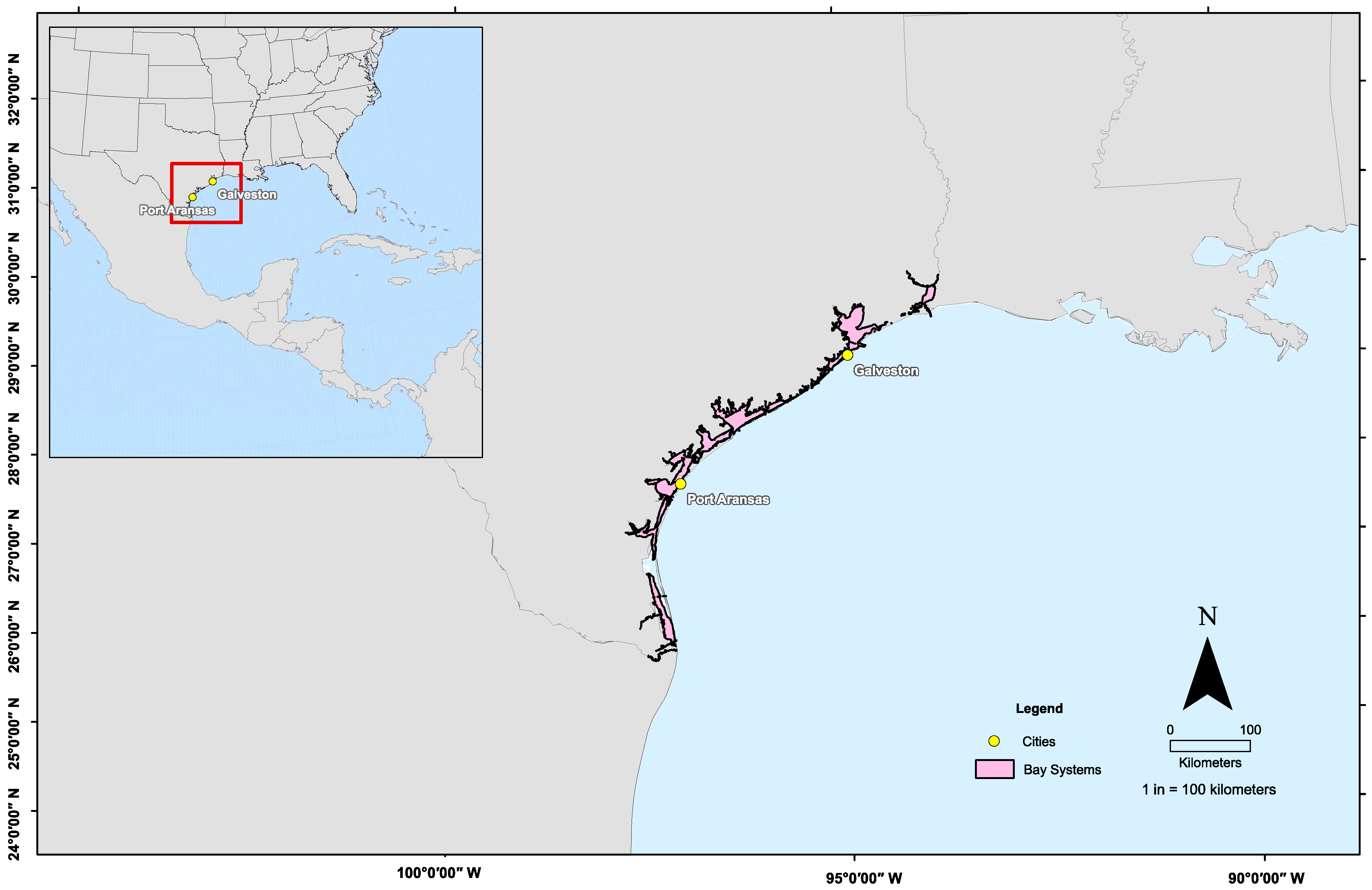
2.1. Sample Collection

The samples for this study were collected from two locations along the upper Texas coast (Galveston, TX, USA) and central Texas coast (Port Aransas, TX, USA) in the northwest Gulf of Mexico (NW GOM) during periods of high fish densities and abundances due to spawning aggregations (Figure 1). Sheepshead were opportunistically collected from recreational fishermen in Galveston (n = 35) and Port Aransas (n = 18) from March to April 2017. Sheepshead were collected from jetties, piers, and nearshore oil rigs, based on post-collection angler surveys. The biological information for each sheepshead collected included sex, weight, and total length (TL). Sex was evaluated by visually examining the gonads from the fish, either being testes (male) or ovaries (female). On site, the stomachs were removed from individuals and immediately placed in Whirl-Paks and stored in a freezer. Epaxial muscle tissue anterior to the primary dorsal fin and a piece of the liver were removed from each fish for the stable isotope analysis and stored in a freezer (−20 °C).

2.2. Analysis of Stomach Contents

Before processing, the stomachs were thawed, preserved via a 48 h fixing process in 10% formalin, and then moved into a solution of 70% ethanol for longer-term storage [21]. Each stomach was weighed for the full wet weight (g) before being opened to weigh (g) all contents separately. Stomach contents assumed to be bait based on angler surveys were not included in our analysis or any subsequent steps. All stomach contents were separated with a mesh sieve (size, 500 μm), and all pieces of bone and carapace were then placed in a petri dish and identified to the lowest possible taxon [21]. For smaller, more numerous taxa (i.e., amphipods), the stomach contents were placed in a gridded petri dish and a subsample (10%) was haphazardly selected for enumeration and taxonomic identification. Once identified, all contents were sorted and then dried at 50 °C for 24 h before weighing to the nearest gram.

2.3. Stable Isotope Analysis

A subset of the fish sampled for stomach contents was used for the stable isotope analysis (Galveston n = 20; Port Aransas n = 18). The sample tissues (muscle and liver) were lyophilized for the stable isotope analysis for 48 h in a FreeZone (Labconco) freeze dryer. Lipids were extracted to remove the confounding effects of lipids on stable isotope values via an Accelerated Solvent Extractor 35 (Dionex). For the lipid extraction process, 34 mL of packed cells were used, with the layered tissue samples being separated by 30 mm filter papers (Whatman). Each extraction cycle ran in 5 min saturations with petroleum ether at 100 °C at 105.5 k/cm2 to reach a thermal equilibrium, followed by a flush with fresh solvent. The lipid extraction procedure was repeated a total of three times per cell to ensure the full removal of lipids. Following the lipid extraction, the tissues were homogenized via a Wig-L-Bug grinding mill and encapsulated in 5 × 9 mm tin capsules, which were placed in a 96-well plate and shipped to the Stable Isotope Facility at the University of California at Davis for the analysis. The samples were weighed for the δ13C and δ15N analyses to the nearest 1 mg, whereas the samples for the δ34S analysis were weighed to the nearest 4 mg. At the stable isotope facility, the analysis of δ13C and δ15N was performed using a PDZ Europa ANCA-GSL elemental analyzer interfaced to a PDZ Europa 20–20 isotope ratio mass spectrometer (IRMS) (Sercon). The sulfur (δ34S) analysis was performed using an Elementar vario ISOTOPE cube interfaced to a 20–22 IRMS (Sercon). For each analysis, the facility compared heavy isotopes with laboratory standards; carbon was compared via Vienna PeeDee Belemnite, nitrogen was compared via atmospheric N2, and sulfur was compared via Vienna Canon Diablo Trilobite. Stable isotope ratios in a delta notation were presented in the following way:
δX = [(Rsample/Rstandard) − 1] × 1000
where X is the heavy isotope, Rsample is the ratio of heavy to light isotopes in the sample, and Rstandard is the ratio of heavy to light isotopes in the reference standard.

2.4. Data Analysis

2.4.1. Analysis of Stomach Contents

Analyses of stomach contents were conducted by organizing the taxonomic groups found in the stomachs into the lowest possible taxon. A percent index of relative importance (%IRI) was computed for prey items using percent weight (%W), percent numerical quantity (%N), and percent frequency of occurrence (%O) [24,25]:
IRI = (%N + %W) × %O
%IRI = (IRIprey/IRItotal) × 100
Square root-transformed Bray–Curtis resemblance matrices of the percent IRI (%IRI) of the stomach contents identified to the broadest relevant taxonomic category were used to estimate the dissimilarity in diets for sheepshead that were caught in Galveston and Port Aransas. For the dissimilarity analyses, ten taxonomic categories were used: amphipoda, annelida, bryozoan, cnidaria, decapoda, isopoda, mollusca, sessilia, plantae, and unidentified material. To determine if sampling was adequate to describe the diets of sheepshead at each location, species accumulation curves were created. Species accumulation curves were created using random starts permuted 999 times, and were presented using a 95% confidence interval. A permutational multivariate analysis of variance (PERMANOVA) was used to compare the square root-transformed diets (%IRI) of individuals collected between the two locations. Due to the asymmetrical sampling of sheepshead between the regions, we concluded that a nonparametric approach such as a PERMANOVA was the most appropriate due to the potentially violated assumptions necessary for the parametric tests. Additionally, to supplement the PERMANOVA analyses and understand the taxonomic differences in the prey found in individual diets, a similarity percentage analysis (SIMPER) was used based on a ranked similarity to identify which prey taxa in the diets drove the dissimilarity between the locations. To determine if the PERMANOVA results were due to dispersion over location effects, each PERMANOVA test was also analyzed using a betadisper analysis. All dietary analyses were conducted using the vegan package v2.5 in R v4.1.3 [26,27].
The trophic position was quantified for sheepshead from both locations using the trophic positions for prey categories estimated in Cortes (1999) [28]. This was achieved by taking the average %IRI for each group (amphipoda, isopoda, etc.) multiplied by the trophic position for each group estimated in Cortes (1999) [28]. Proportional trophic positions for all groups were then summed to estimate the trophic positions for the sheepshead at each location.

2.4.2. Stable Isotope Analysis

A multivariate analysis of variance (MANOVA) was used to test for differences in the δ13C, δ15N, and δ34S stable isotope values between the sample locations and tissue type. The influence of the independent variables (location and tissue type) was examined for each of the dependent variables (δ13C, δ15N, and δ34S) using a one-way analysis of variance (ANOVA). The significance of the statistical testing was determined at a value of p ≤ 0.05. Prior to the analysis, data for each stable isotope ratio (δ13C, δ15N, and δ34S) for each factor were found to normally distributed and homoscedastic, meeting the assumptions for the parametric analyses.
The trophic niche overlap was estimated for each location and tissue sample using a combination of δ13C, δ15N, and δ34S. Using a Bayesian framework, three-dimensional probabilistic regions that represented 95% of the total niche area were identified with clustering using the nicheRover package [29]. The niche size was estimated using 10,000 Monte Carlo estimates to derive posterior means and 95% credible intervals, followed by an estimation of the niche size by location overlap with an additional Monte Carlo procedure (n = 10,000), where random pairs of niche spaces were compared with the estimate overlap between locations. All analyses were undertaken in R v4.1.3 [27].

3. Results

3.1. Stomach Contents

Of the 53 total stomachs examined (Galveston, n = 35 and Port Aransas, n = 18), 26 of the sheepshead caught in Galveston and 12 from Port Aransas contained identifiable prey items that were used for the statistical analysis. Along with stomachs, a subset of sheepshead tissue samples (Galveston n = 20; Port Aransas n = 18) was also analyzed for stable isotopes. The size ranges and sex ratios varied for the samples from both locations. Sheepshead collected from Galveston ranged from 370 to 506 mm in total length (TL) (18 females (means ± SD), TL = 437.5 ± 34.6 mm; 17 males, TL 410.8 ± 33.1 mm) and samples collected from Port Aransas ranged from 320 to 488 mm in TL (12 females, TL = 397.2 ± 45.3 mm; 11 males, TL 406.5 ± 32.9 mm). All fish caught were adult sheepshead, based on a visual assessment of the gonadal stage, and were larger than the average length at sexual maturity [30].
The percent index of relative importance (%IRI) of the sheepshead diet was similar at both locations based on the taxonomic group, with amphipods being one of the most influential prey items (Table 1). The stomach contents of sheepshead from Galveston primarily comprised amphipods (%IRI = 61.79), with the families Caprellidae and Corophiidae (%IRICaprellidae = 30.68; %IRICorophiidae = 24.38) making up most of the amphipods found. Decapods (%IRI = 7.29) were the second major contributor to sheepshead from Galveston. However, barnacles were the largest contributor to sheepshead from Port Aransas (%IRI = 39.53), with amphipods as their second major contributor (%IRI = 30.19) and decapods as their third identifiable prey (%IRI = 8.03), aside from unidentified matter (%IRI = 16.48) (Table 1).
A total of nine taxonomic groups were identified through an analysis of the stomach contents. Significant differences were observed in the dietary composition of sheepshead collected from the two locations. The PERMANOVA revealed differences between the two locations (F = 14.33; p = 0.001), indicating that the sheepshead collected within each location had different diets from one another. The PERMDISP test for dispersion was nonsignificant (PERMDISP, F = 3.16; p = 0.089), thereby suggesting that the differences observed with the PERMANOVA were due to a location effect rather than dispersion.
The SIMPER analysis showed that amphipods, barnacles, unidentified prey, isopoda, and algae contributed the most to the differences in the diet of sheepshead at each location. In terms of %IRI, amphipods were the main group that drove the differences in the overall diet composition between the sheepshead from both locations. Amphipods made up 36% of the differences between the sheepshead from Galveston and Port Aransas. Barnacles were the second major group, which made up 29% of the dissimilarities; then unidentified material, with 17% dissimilarity; then isopoda (7% dissimilarity) and algae (6% dissimilarity). The rest of the groups found in sheepshead stomachs differed by ≤5% dissimilarity.
The trophic positions (TP) for sheepshead caught in Galveston (TP = 1.99) were estimated using identified prey from the stomach contents and were slightly higher than Port Aransas (TP = 1.83). The TP calculations for the sheepshead were considerably dependent on primary and secondary consumers.

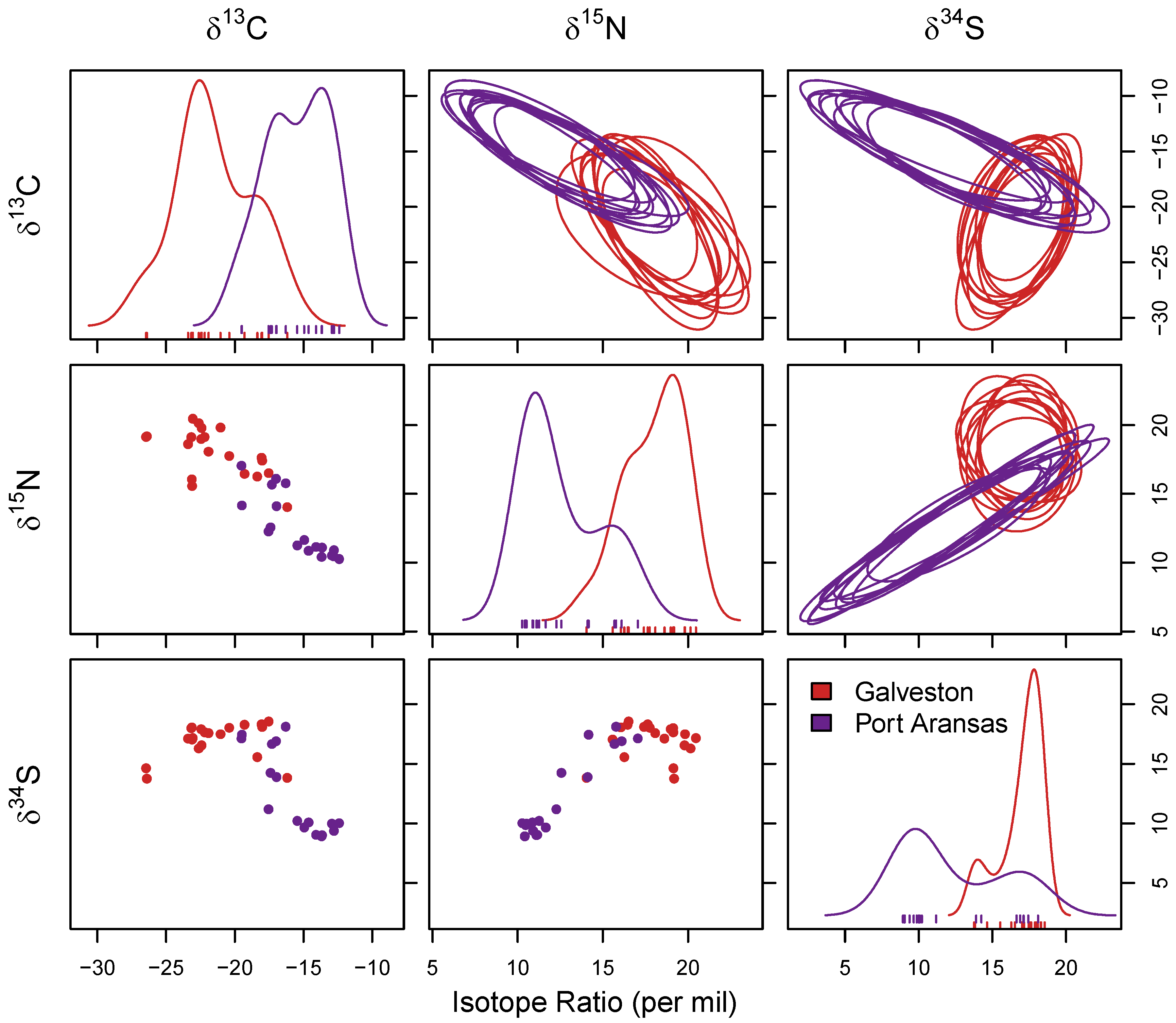
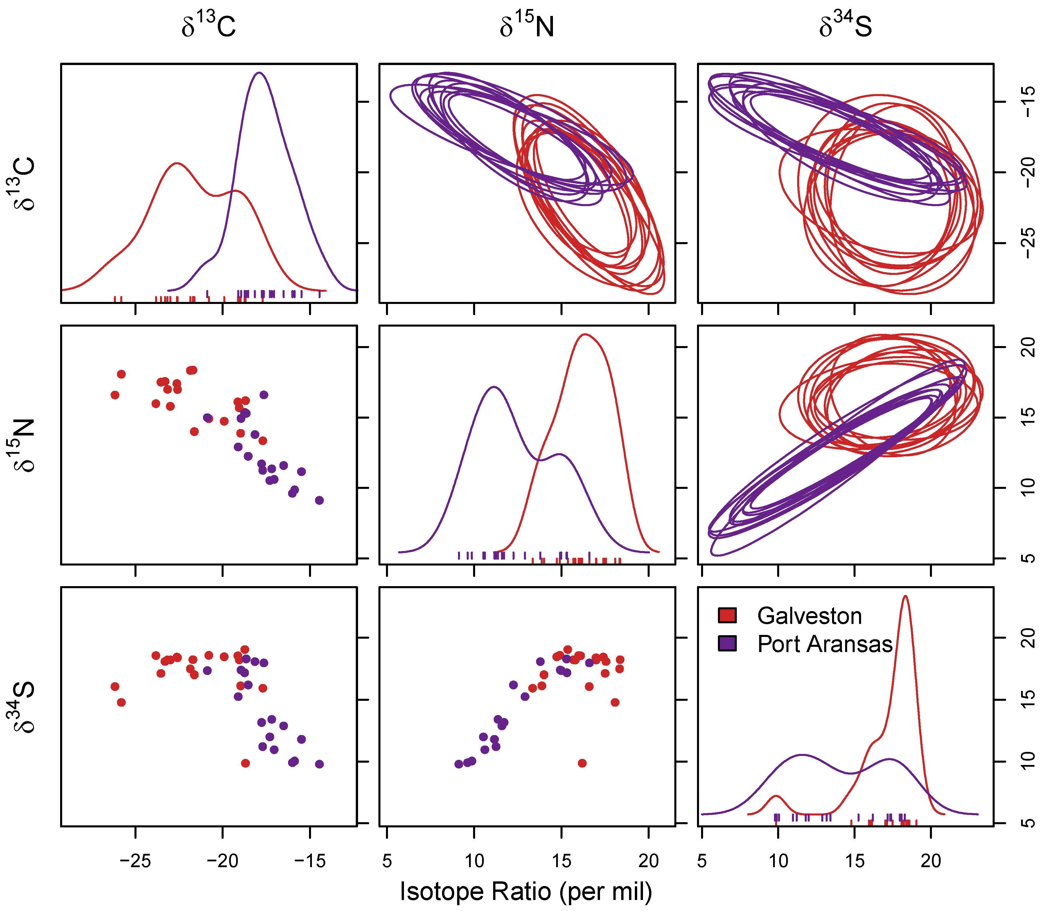
3.2. Stable Isotope Analysis

The results of the MANOVA revealed significant differences in δ13C, δ15N, and δ34S stable isotope values from the muscle tissue of sheepshead in relation to the collection location. Significant differences existed (F1,36 = 22.95; p < 0.05) in the stable isotope ratios (δ13C, δ15N, and δ34S) in the muscle samples for the sheepshead from both locations. The δ13C values indicated a significant difference between locations (F1,36 = 50.80; p < 0.05), with lower δ13C values in the muscle samples of the sheepshead from Galveston ((mean ± SD) −21.46 ± 2.81‰) relative to Port Aransas (−15.50 ± 2.28‰) (Figure 2). The δ15N values were also significantly different in the muscle samples of sheepshead between both locations (F1,36 = 69.08; p < 0.05), with higher δ15N values in the sheepshead from Galveston (18.01 ± 1.74‰) than from Port Aransas (12.57 ± 2.28‰) (Figure 2). Additionally, δ34S had significantly different values at both locations (F1,36 = 30.27; p < 0.05), with higher δ34S values in the muscle samples from the sheepshead collected in Galveston (16.98 ± 1.46‰) than Port Aransas (12.31 ± 3.47‰) (Figure 2).
The same analysis was conducted to test for differences in the δ13C, δ15N, and δ34S stable isotope values found in the liver samples. Similar to the muscle samples, significant differences were found (F1,38 = 16.83; p < 0.05) in the liver samples between the locations. The δ13C values indicated a significant difference between locations (F1,38 = 42.89; p < 0.05), with lower δ13C values in the liver samples in the sheepshead from Galveston (−21.60 ± 2.42‰) than Port Aransas (−17.56 ± 1.53‰) (Figure 3), mirroring the results found in the muscle samples. The δ15N values were also significantly different between locations (F1,38 = 44.20; p < 0.05), with higher δ15N values in the liver samples from the sheepshead collected in Galveston (16.19 ± 1.49‰) relative to Port Aransas (12.38 ± 2.25‰) (Figure 3). Furthermore, the δ34S values were significantly different between both locations (F1,38 = 17.71; p < 0.05), with higher δ34S values in the liver samples found in the sheepshead from Galveston (17.27 ± 2.08‰) compared with Port Aransas (14.05 ± 3.15‰) (Figure 3). The overall results supported the differences in stable isotope values between the locations, with the δ13C values being lower in both the muscle and liver samples from the sheepshead collected in Galveston relative to Port Aransas, whereas the δ15N and δ34S values were higher in both the muscle and liver samples from the sheepshead collected in Galveston relative to Port Aransas.

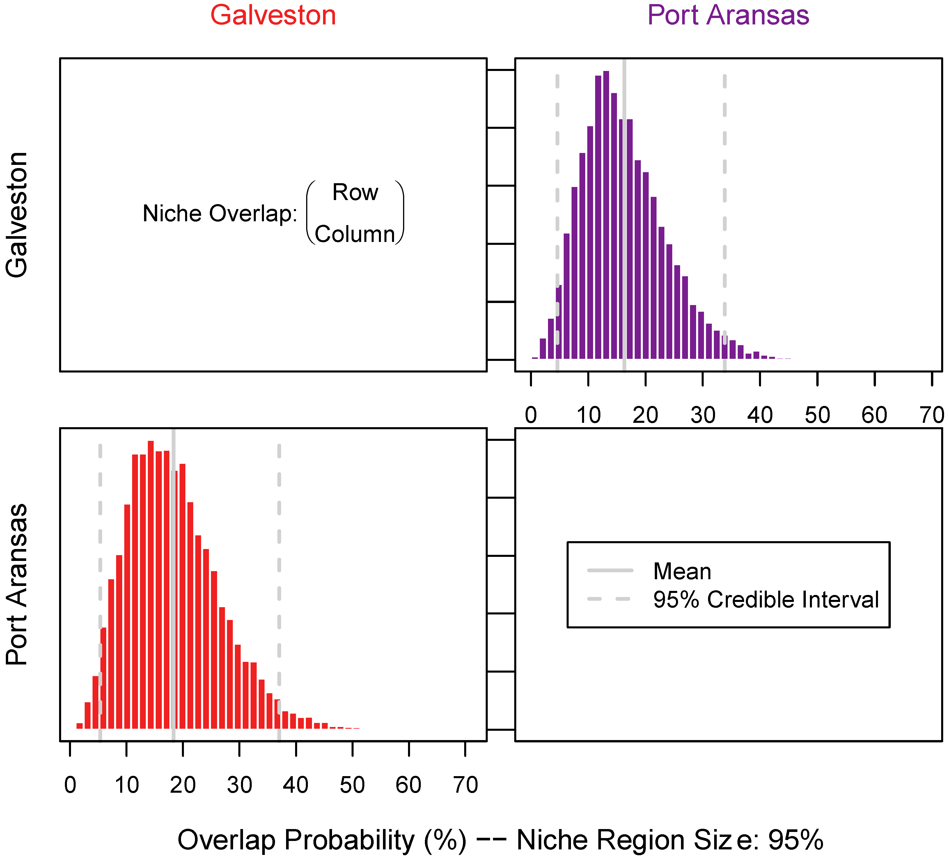
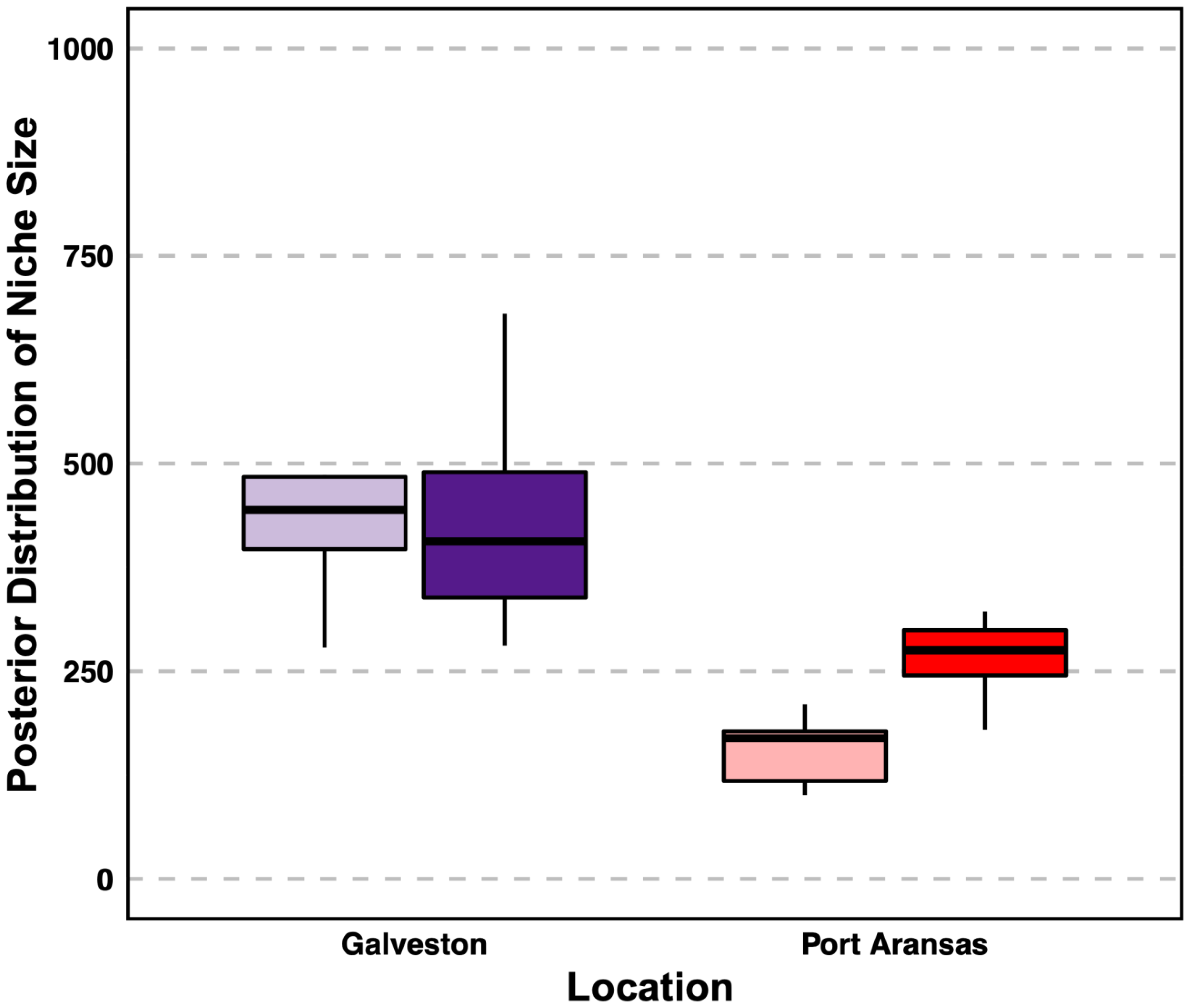
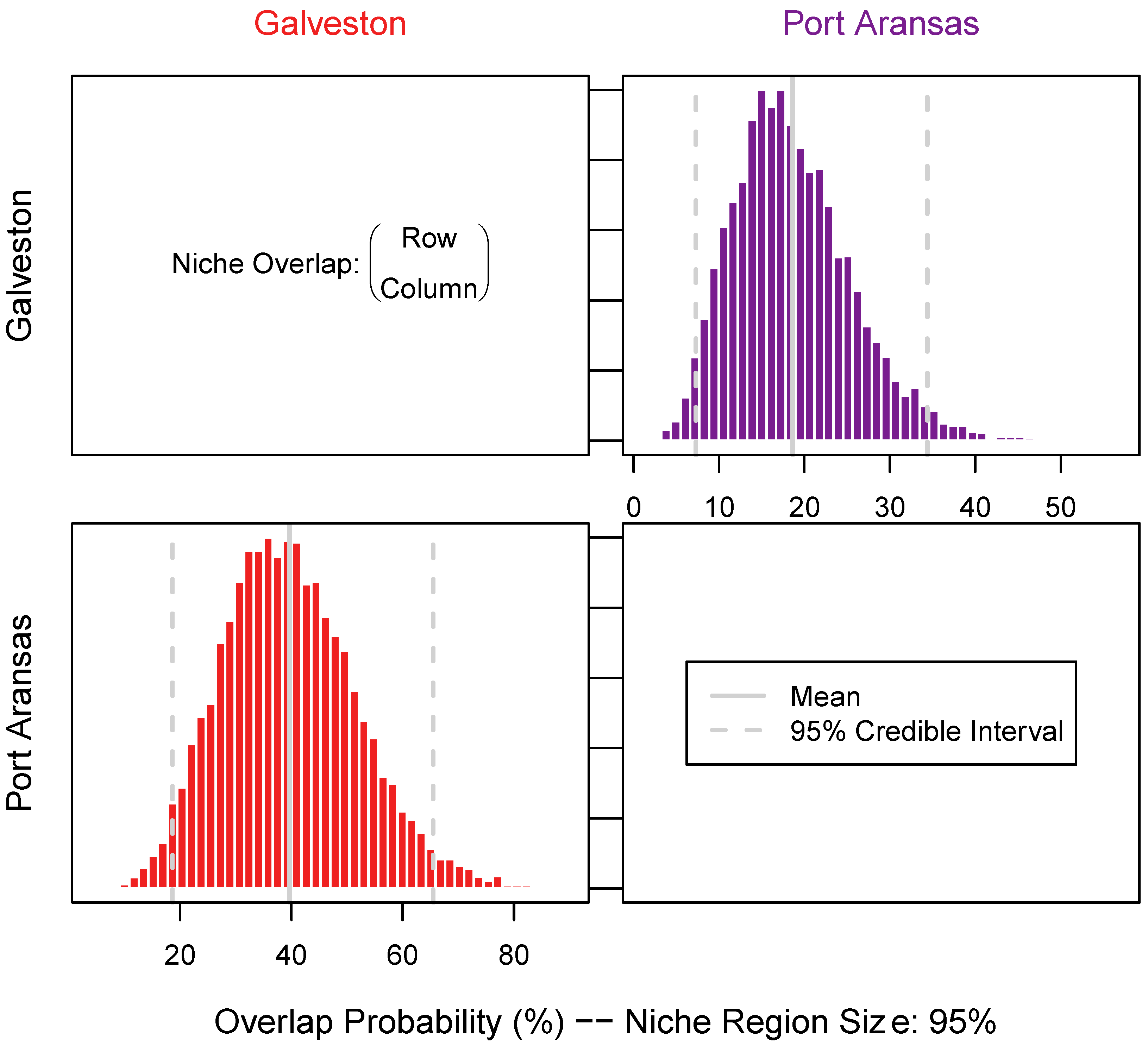
3.3. Niche Size and Overlap

The niche size was defined by δ13C, δ15N, and δ34S and varied between the sheepshead from both locations and the tissue types. Galveston sheepshead consisted of a larger niche size in the muscle (long-term turnover) samples ((mean + SD) 479.3 ± 131.2) than Port Aransas (178.8 ± 54.3) (Figure 4 and Figure 5). Similarly, the Galveston sheepshead niche size in the liver (short-term turnover) samples were larger (433.3 ± 120.3) than those from Port Aransas (270.0 ± 80.9) (Figure 4 and Figure 6). The niche overlap also varied among the location and tissue type of the sheepshead. The sheepshead from Galveston overlapped with the sheepshead from Port Aransas in the muscle samples by 16.47% (CI2.5 = 6; CI97.5 = 37), whereas the sheepshead from Port Aransas overlapped with the sheepshead from Galveston by 18.49% (CI2.5 = 4; CI97.5 = 34) (Figure 5 and Figure 6). In the liver samples, the sheepshead from Galveston overlapped with the sheepshead from Port Aransas by 18.56% (CI2.5 = 18; CI97.5 = 65), whereas the sheepshead from Port Aransas overlapped with the sheepshead from Galveston by 39.17% (CI2.5 = 7; CI97.5 = 35) (Figure 5 and Figure 6).

4. Discussion

This study examined the trophic interactions and feeding ecology of sheepshead from two different locations on the Texas coast in the NW GOM. Our results highlight the importance of small benthic invertebrates (e.g., amphipods and decapods) in the diet of sheepshead. The findings from this study were consistent with previous studies [6,7,14,15,23,31,32], where examinations of sheepshead stomach contents showed that sheepshead primarily forage on amphipods, barnacles, and plant matter. Multiple species of amphipods made up the majority of the prey items in the sheepshead from Galveston (%IRI = 61.79), whereas barnacles were the primary diet item for the sheepshead collected in Port Aransas (%IRI = 39.53). We estimated a higher trophic position for the sheepshead caught in Galveston (TP = 1.99) than Port Aransas (TP = 1.83) by a value of 0.16, using identified prey from the stomach contents. The differences between the sheepshead from Galveston and the sheepshead from Port Aransas were visible in δ13C, δ15N, and δ34S, which persisted in both the muscle and liver. δ13C was lower, and δ15N and δ34S were higher in the samples from Galveston than Port Aransas. A disparity in δ13C values was previously observed by TinHan and Wells (2021) [33], where they observed values of δ13C having latitudinal trends increasing from north to south. This was similar to our study, which showed that the δ13C values in Galveston were much lower than those in Port Aransas. Discrepancies can be driven by numerous factors such as the consumption/assemblage of prey, location differences of primary production sources, and trophic level [33].
In this study, the main prey organism of the sheepshead collected from Galveston was amphipods, whereas barnacles were the main prey for the conspecifics collected from Port Aransas. The differences in the overall prey assemblage in the sheepshead stomachs from both locations were congruent with those of Cutwa and Turingan’s (2000) [23] study of sheepshead from two distinct locations in a Florida estuary. Cutwa and Turingan (2000) [23] observed a difference in the consumption of hard-body prey organisms (barnacles) between locations. Differences in the prey assemblage between locations could be attributed to abiotic factors such as salinity, dissolved oxygen, depth, sediment, upwelling, estuarine runoff, or temperature as they have been observed to play critical roles in the biomass and density of marine organisms in platforms found in the GOM [31,34,35,36,37,38,39]. A lower salinity in Galveston than Port Aransas [40] could explain the differences in the fouling communities present at each location and, thus, the trophic position of the sheepshead. Consequently, general inferences on the feeding style of sheepshead could be made based on the stomach contents from both locations. Sheepshead from Galveston feeding primarily on amphipods could reflect a greater benthic contribution because amphipods have been recorded in benthic habitats in the GOM [41]. In contrast, the Port Aransas sheepshead showed more suspension feeding due to feeding more heavily on barnacles, which tend to be higher in the water column attached to platforms [22]. However, sheepshead have been documented to forage in and near oil and gas platforms [6] and in nearshore and offshore habitats [7,15], but they are found in most habitats in the GOM, including brackish estuaries, bayous, and saltwater bays or structures with marine growth [3]. In this study, the sheepshead were caught in a variety of habitats and artificial reefs in nearshore and offshore ecosystems, so it was not possible to make a direct habitat link.
Although habitat types and environmental conditions influence the type of prey assemblage found, they also influence the trophic position due to changes in foraging, prey variation, abundance, and diversity [42,43,44,45,46]. The GOM has many artificial reefs that serve as important habitats for marine fish that also function as important foraging grounds [6,47]. Artificial reefs such as jetties and oil platforms provide habitats and foraging locations for both sessile and mobile organisms that sheepshead are known to prey on. Most of these structures consist of piles of unconsolidated rocks and rubble, which provide fish with equal or greater refuge from predation than naturally occurring reefs [48,49]. Furthermore, the biodiversity and abundance of epibiota and sessile organisms (i.e., algae, oysters, mussels, and barnacles) are not inherently different from natural shorelines [48]. Therefore, nearshore protection structures provide similar ecological services to epibiota communities, which in turn provide resources to commercially and recreationally important fish species [17,49,50,51], including sheepshead.
The isotopic signatures varied between locations (Galveston and Port Aransas) and by tissue (muscle and liver) samples for the sheepshead. δ13C was highest in the sheepshead samples from Port Aransas, where the waters have a higher salinity than in Galveston. A positive relationship between salinity and measures of δ13C has been reported in previous studies [52,53]. The positive relationship between salinity and δ13C along the coast of Texas is likely caused the by freshwater inflow and terrestrial carbon that increase the δ13C in the dissolved inorganic carbon pool [53]. It has been documented in other studies that salinity increases from north to south in the Texas region, explaining the lower salinity gradient found in Galveston than Port Aransas [40]. Similarly, seagrass coverage (13C-enriched producers) also increases from north to south, which could cause the δ13C values to be higher in Port Aransas [53]. In northern regions such as Galveston, much of the organic matter is derived from phytoplankton or other sources of primary production such as salt-marsh plants or algae [53]. However, the lower δ13C values in Galveston sheepshead could also be explained by the salinity and estuarine runoff, which have been linked to an influence in isotope composition [53]. Although we did not directly measure salinity or other environmental parameters, the mean salinity differed between the two study locations [54].
However, the δ13C and δ15N values were higher in the muscle samples than the liver samples for the sheepshead from both locations, whereas the δ34S values were higher in the liver samples than the muscle samples, suggesting a landward–seaward movement [55]. As mentioned earlier, the waters surrounding Port Aransas are more saline than those surrounding Galveston, and there is substantially less freshwater input into the water surrounding Port Aransas [40]. It has been documented that consumers exhibit variable δ15N values, which are associated with salinity [56]. Matich et al. (2021) [56] found that there was a negative relationship between δ15N and salinity in areas where 15N-enriched nitrogen was increased, indicating that 15N-enriched nitrogen may influence the base of food webs. Similarly, the values of δ15N varied among the estuaries sampled in the Gulf of Mexico, which may explain the differences observed in this study [33]. Estuarine ecotones such as those created at the interface of freshwater and saltwater are related to substantially higher biodiversity than marine water or freshwater alone [57]. If sheepshead do make a landward to seaward shift at either location (Galveston or Port Aransas), as the δ34S isotopic values suggest, sheepshead could be traversing this ecotone to areas of differing biodiversity, specifically as they relate to the sheepshead’s prey field. Understanding this movement is especially important when evaluating the ecological roles that sheepshead play—specifically, during annual spawning aggregations—and should be an area of future study.
The isotopic niche size and overlap varied between the sheepshead from both locations and tissue types, which may be an indication of differences in the relative abundance of prey and migration of sheepshead. Sheepshead are omnivores that feed primarily on invertebrates [1,23] and occasionally small vertebrates and plant matter [23,58,59]. As the generalized diets of sheepshead are related to the regional community composition of the benthic prey assemblage, regional differences in the assemblage may explain why the Galveston specimens had larger isotopic niches in the muscle (by 3%) and liver (by 1.6%) samples than Port Aransas. The proportionally low overlap (muscle average, 25.72% and liver average, 38.15%) in the isotopic niche between the regions was surprising given the relative importance of similar prey items, although this may be attributed to the difference in dominant prey items between regions or migratory behavior. Differences in prey items may be due to regional environmental differences in primary production at the base of food webs, as mentioned previously. Between the short-term turnover tissues (liver) and long-term turnover tissues (muscle), there was an apparent niche contraction from long-term to short-term for the Galveston samples (479.3 muscle and 433.3 liver; Δ = −9.6%). This was reversed for Port Aransas, where the sheepshead niche expanded from the long-term to the short-term (178.8 muscle and 270.0 liver; Δ = 51%). This may also be due to the differences in foraging locations between Galveston Bay and Port Aransas.

5. Conclusions

In conclusion, the feeding patterns measured using stomach contents and stable isotope values differed between sheepshead from Galveston and Port Aransas, similar to other studies that observed sheepshead collected from different locations [6,7,14,15,23,31,32]. Potentially, sheepshead feed heavily at spawning sites for months before they begin to spawn and continue to do so during the spawning season. This study showed the diet composition of sheepshead during the spawning season, but the differences observed in this study could be temporally broad due to diet changes that occur from December, when they begin to aggregate for the spawning season. Therefore, a more structured, spatiotemporal study may elucidate finer-scale ontogenetic shifts in diet in relation to spawning.

Author Contributions

Conceptualization, all; methodology, all; formal analysis, all; investigation, all; data curation, E.M.G. and J.D.P.; writing—original draft preparation, all; writing—review and editing, all; project visualization, E.M.G. and J.D.P. All authors have read and agreed to the published version of the manuscript.

Funding

This research was funded in part by the Louis Stokes Alliance for Minority Participation (LSAMP) at Texas A&M University at Galveston.

Institutional Review Board Statement

For this study, an ethics review and collection permit were not needed.

Data Availability Statement

Data are available upon request to the corresponding author.

Acknowledgments

We would like to thank members of the Shark Biology and Fisheries Science Laboratory at Texas A&M University at Galveston and the Marine Science Institute at The University of Texas, Austin, for their help in the sampling and processing of the samples for this project. We would also like to thank David and Beverley Barfield and their friends for donating sheepshead carcasses to this study. Additionally, we thank the Louis Stokes Alliance for Minority Participation (LSAMP) for their financial resources.

Conflicts of Interest

The authors declare no conflict of interest.

References

  1. Fernandez, L.P.H.; Motta, P.J. Trophic consequences of differential performance: Ontogeny of oral jaw-crushing performance in the sheepshead, Archosargus probatocephalus (Teleostei, Sparidae). J. Zool. 1997, 243, 737–756. [Google Scholar] [CrossRef]
  2. Personal Communication from the National Marine Fisheries Service; NOAA Fisheries, Fisheries Statistics Division: Silver Spring, MD, USA, 2013. Available online: https://www.fisheries.noaa.gov/foss/f?p=215:200:15293546732758:Mail:::: (accessed on 17 December 2022).
  3. VanderKooy, S.J. (Ed.) The Sheepshead Fishery of the Gulf of Mexico, United States: A Fisheries Profile; Gulf States Marine Fisheries Commission: Ocean Springs, MS, USA, 2006; Publication Number 143; 176p. [Google Scholar]
  4. Johnson, G.D. Development of Fishes of the Mid-Atlantic Bight: An Atlas of Egg, Larval, and Juvenile Stages. In Carangidae through Ephippidae; U.S. Fish and Wildlife Service: Washington, DC, USA, 1978; Volume 4. [Google Scholar]
  5. Nelson, J.S.; Grande, T.C.; Wilson, M.V.H. Fishes of the World; Wiley: Hoboken, NJ, USA, 2016. [Google Scholar]
  6. Reeves, D.B.; Chesney, E.J.; Munnelly, R.T.; Baltz, D.M. Sheepshead Foraging Patterns at Oil and Gas Platforms in the Northern Gulf of Mexico. N. Am. J. Fish. Manag. 2018, 38, 1258–1274. [Google Scholar] [CrossRef]
  7. Sedberry, G.R. Feeding Habits of Sheepshead, Archosargus probatocephalus, in Offshore Reef Habitats of the Southeastern Continental Shelf. Gulf Mex. Sci. 1987, 9, 3. [Google Scholar] [CrossRef] [Green Version]
  8. Ballenger, J.C. Population Dynamics of Sheepshead (Archosargus probatocephalus; Walbaum 1792) in the Chesapeake Bay Region: A comparison to Other Areas and an Assessment of Their Current Status. Ph.D. Thesis, Old Dominion University, Norfolk, VA, USA, 2011. [Google Scholar] [CrossRef]
  9. Wenner, C.A.; Archambault, J. Sheepshead: The Natural History and Fishing Techniques in South Carolina; Charleston, SC Marine Resources Research Institute, Marine Resources Division, South Carolina Wildlife and Marine Resources Department: Charleston, SC, USA, 2006; p. 48.
  10. Dutka-Gianelli, J.; Murie, D. Age and growth of sheepshead, Archosargus probatocephalus (Pisces: Sparidae), from the northwest coast of Florida. Bull. Mar. Sci. 2001, 68, 69–83. [Google Scholar]
  11. Jennings, C.A. Species Profiles: Life Histories and Environmental Requirements of Coastal Fishes and Invertebrates (Gulf of Mexico): Sheepshead; The Service: Washington, DC, USA, 1985. [Google Scholar]
  12. Biggs, C.R.; Heyman, W.D.; Farmer, N.A.; Kobara, S.I.; Bolser, D.G.; Robinson, J.; Lowerre-Barbieri, S.K.; Erisman, B.E. The importance of spawning behavior in understanding the vulnerability of exploited marine fishes in the US Gulf of Mexico. PeerJ 2021, 9, e11814. [Google Scholar] [CrossRef]
  13. Helies, F.C.; Jamison, J.L. Prediction and Verification of Snapper-Grouper Spawning Aggregation Sites on the Offshore Banks of the Northwestern Gulf of Mexico; Final Report for Gulf and Atlantic Fisheries Foundation Inc.: Tampa, FL, USA; Gulf and Atlantic Fisheries Foundation Inc.: Tampa, FL, USA, 2016. [Google Scholar]
  14. Springer, V.G.; Woodburn, K.D. An Ecological Study of the Fishes of the Tampa Bay Area; Florida State Board of Conservation, Marine Laboratory: St. Petersburg, FL, USA, 1960. [Google Scholar]
  15. Heil, A.D. Life History, Diet, and Reproductive Dynamics of the Sheepshead (Archosargus probatocephalus) in the Northeastern Gulf of Mexico. Master’s Thesis, Florida State University, Tallahassee, FL, USA, 2017. [Google Scholar]
  16. Cresson, P.; Ruitton, S.; Harmelin-Vivien, M. Artificial reefs do increase secondary biomass production: Mechanisms evidenced by stable isotopes. Mar. Ecol. Prog. Ser. 2014, 509, 15–26. [Google Scholar] [CrossRef]
  17. Daigle, S.T.; Fleeger, J.W.; Cowan, J.H., Jr.; Pascal, P.-Y. What Is the Relative Importance of Phytoplankton and Attached Macroalgae and Epiphytes to Food Webs on Offshore Oil Platforms? Mar. Coast. Fish. 2013, 5, 53–64. [Google Scholar] [CrossRef]
  18. Dance, K.M.; Rooker, J.R.; Shipley, J.B.; Dance, M.A.; Wells, R.J.D. Feeding ecology of fishes associated with artificial reefs in the northwest Gulf of Mexico. PLoS ONE 2018, 13, e0203873. [Google Scholar] [CrossRef] [Green Version]
  19. Michener, R.; Lajtha, K. Stable Isotopes in Ecology and Environmental Science; John Wiley & Sons: Hoboken, NJ, USA, 2008. [Google Scholar]
  20. Peterson, B.J.; Fry, B. Stable Isotopes in Ecosystem Studies. Annu. Rev. Ecol. Syst. 1987, 18, 293–320. [Google Scholar] [CrossRef]
  21. Plumlee, J.D.; Wells, R.J.D. Feeding ecology of three coastal shark species in the northwest Gulf of Mexico. Mar. Ecol. Prog. Ser. 2016, 550, 163–174. [Google Scholar] [CrossRef] [Green Version]
  22. Reeves, D.B.; Chesney, E.J.; Munnelly, R.T.; Baltz, D.M.; Maiti, K. Trophic Ecology of Sheepshead and Stone Crabs at Oil and Gas Platforms in the Northern Gulf of Mexico’s Hypoxic Zone. Trans. Am. Fish. Soc. 2019, 148, 324–338. [Google Scholar] [CrossRef]
  23. Cutwa, M.M.; Turingan, R.G. Intralocality Variation in Feeding Biomechanics and Prey Use in Archosargus probatocephalus (Teleostei, Sparidae), with Implications for the Ecomorphology of Fishes. Environ. Biol. Fishes 2000, 59, 191–198. [Google Scholar] [CrossRef]
  24. Cortés, E. A critical review of methods of studying fish feeding based on analysis of stomach contents: Application to elasmobranch fishes. Can. J. Fish. Aquat. Sci. 1997, 54, 726–738. [Google Scholar] [CrossRef]
  25. Pinkas, L.; Oliphant, M.S.; Iverson, I.L. Food Habits of Albacore, Bluefin Tuna and Bonito in California Waters; Fish Bulletin 152; UC San Diego Library: San Diego, CA, USA, 1970; pp. 1–139. [Google Scholar]
  26. Oksanen, J.; Blanchet, F.G.; Kindt, R.; Legendre, P.; Minchin, P. The Vegan Package: Community Ecology Package, R Package Version 2.0–2; R Core Team: Vienna, Austria, 2011. [Google Scholar]
  27. R Core Team. R: A Language and Environment for Statistical Computing; R Core Team: Vienna, Austria, 2022. [Google Scholar]
  28. Cortés, E. Standardized diet compositions and trophic levels of sharks. ICES J. Mar. Sci. 1999, 56, 707–717. [Google Scholar] [CrossRef]
  29. Swanson, H.K.; Lysy, M.; Power, M.; Stasko, A.D.; Johnson, J.D.; Reist, J.D. A new probabilistic method for quantifying n-dimensional ecological niches and niche overlap. Ecology 2015, 96, 318–324. [Google Scholar] [CrossRef] [PubMed]
  30. Biggs, C.; Erisman, B.; Heyman, W.; Kobara, S.; Farmer, N.; Lowerre-Barbieri, S.K.; Karnauskas, M.; Brenner, J. Fish Spawning Aggregations and Fisheries in the Gulf of Mexico: Interactions, Data Gaps and Research Priorities. In Proceedings of the 147th Annual Meeting of the American Fisheries Society, Tampa, FL, USA, 20–24 August 2017. [Google Scholar]
  31. Odum, W.E.; Heald, E.J. Trophic analyses of an estuarine mangrove community. Bull. Mar. Sci. 1972, 22, 671–738. [Google Scholar]
  32. Randall, J.E. Food Habits of Reef Fishes of the West Indies; Institute of Marine Sciences, University of Miami: Miami, FL, USA, 1967; Volume 5, pp. 665–847. [Google Scholar]
  33. TinHan, T.C.; Wells, R.D. Spatial and ontogenetic patterns in the trophic ecology of juvenile Bull Sharks (Carcharhinus leucas) from the Northwest Gulf of Mexico. Front. Mar. Sci. 2021, 8, 664316. [Google Scholar] [CrossRef]
  34. Egerton, J.P.; Bolser, D.G.; Grüss, A.; Erisman, B.E. Understanding patterns of fish backscatter, size and density around petroleum platforms of the US Gulf of Mexico using hydroacoustic data. Fish. Res. 2021, 233, 105752. [Google Scholar] [CrossRef]
  35. Hooper, D.U.; Chapin, F.S., III; Ewel, J.J.; Hector, A.; Inchausti, P.; Lavorel, S.; Lawton, J.H.; Lodge, D.M.; Loreau, M.; Naeem, S.; et al. Effects of biodiversity on ecosystem functioning: A consensus of current knowledge. Ecol. Monogr. 2005, 75, 3–35. [Google Scholar] [CrossRef]
  36. Palardy, J.E.; Witman, J.D. Water flow drives biodiversity by mediating rarity in marine benthic communities. Ecol. Lett. 2011, 14, 63–68. [Google Scholar] [CrossRef] [PubMed]
  37. Reynolds, E.M.; Cowan, J.H.; Lewis, K.A.; Simonsen, K.A. Method for estimating relative abundance and species composition around oil and gas platforms in the northern Gulf of Mexico, USA. Fish. Res. 2018, 201, 44–55. [Google Scholar] [CrossRef]
  38. Wilson, C.A.; Nieland, D.L. Age and growth of red snapper, Lutjanus campechanus, from the Northern Gulf of Mexico off Louisiana. Fish. Bull. 2001, 99, 653–665. [Google Scholar]
  39. Worm, B.; Barbier, E.B.; Beaumont, N.; Duffy, J.E.; Folke, C.; Halpern, B.S.; Jackson, J.B.C.; Lotze, H.K.; Micheli, F.; Palumbi, S.R.; et al. Impacts of Biodiversity Loss on Ocean Ecosystem Services. Science 2006, 314, 787. [Google Scholar] [CrossRef] [Green Version]
  40. Tolan, J.M. El Niño-Southern Oscillation impacts translated to the watershed scale: Estuarine salinity patterns along the Texas Gulf Coast, 1982 to 2004. Estuar. Coast. Shelf Sci. 2007, 72, 247–260. [Google Scholar] [CrossRef]
  41. Winfield, I.; Escobar-Briones, E.; Morrone, J.J. Updated checklist and identification of areas of endemism of benthic amphipods (Caprellidea and Gammaridea) from offshore habitats in the SW Gulf of Mexico. Sci. Mar. 2006, 70, 99–108. [Google Scholar] [CrossRef]
  42. Gibb, H.; Cunningham, S.A. Habitat contrasts reveal a shift in the trophic position of ant assemblages. J. Anim. Ecol. 2011, 80, 119–127. [Google Scholar] [CrossRef]
  43. Lei, J.; Jia, Y.; Wang, Y.; Lei, G.; Lu, C.; Saintilan, N.; Wen, L.I. Behavioural plasticity and trophic niche shift: How wintering geese respond to habitat alteration. Freshw. Biol. 2019, 64, 1183–1195. [Google Scholar] [CrossRef]
  44. Moosmann, M.; Cuenca-Cambronero, M.; De Lisle, S.; Greenway, R.; Hudson, C.M.; Lürig, M.D.; Matthews, B. On the evolution of trophic position. Ecol. Lett. 2021, 24, 2549–2562. [Google Scholar] [CrossRef] [PubMed]
  45. Tewfik, A.; Bell, S.S.; McCann, K.S.; Morrow, K. Predator diet and trophic position modified with altered habitat morphology. PLoS ONE 2016, 11, e0147759. [Google Scholar] [CrossRef]
  46. Van Rijssel, J.C.; Hecky, R.E.; Kishe-Machumu, M.A.; Witte, F. Changing ecology of Lake Victoria cichlids and their environment: Evidence from C13 and N15 analyses. Hydrobiologia 2017, 791, 175–191. [Google Scholar] [CrossRef] [Green Version]
  47. Reeds, K.A.; Smith, J.A.; Suthers, I.M.; Johnston, E.L. An ecological halo surrounding a large offshore artificial reef: Sediments, infauna, and fish foraging. Mar. Environ. Res. 2018, 141, 30–38. [Google Scholar] [CrossRef]
  48. Clynick, B.; Chapman, M.G.; Underwood, A. Effects of epibiota on assemblages of fish associated with urban structures. Mar. Ecol. 2007, 332, 201–210. [Google Scholar] [CrossRef] [Green Version]
  49. Gittman, R.K.; Scyphers, S.B.; Smith, C.S.; Neylan, I.P.; Grabowski, J.H. Ecological Consequences of Shoreline Hardening: A Meta-Analysis. BioScience 2016, 66, 763–773. [Google Scholar] [CrossRef] [Green Version]
  50. Reeves, D.B. The Influence of River Discharge on Fishes and Invertebrates Associated with Small Oil and Gas Platforms in Nearshore Louisiana. Ph.D. Thesis, Louisiana State University, Baton Rouge, LA, USA, 2018. [Google Scholar]
  51. Schulze, A.; Erdner, D.L.; Grimes, C.J.; Holstein, D.M.; Miglietta, M.P. Artificial Reefs in the Northern Gulf of Mexico: Community Ecology Amid the “Ocean Sprawl”. Front. Mar. Sci. 2020, 7, 447. [Google Scholar] [CrossRef]
  52. Kerr, L.A.; Secor, D.H.; Kraus, R.T. Stable isotope (δ13C and δ18O) and Sr/Ca composition of otoliths as proxies for environmental salinity experienced by an estuarine fish. Mar. Ecol. Prog. Ser. 2007, 349, 245–253. [Google Scholar] [CrossRef]
  53. Rooker, J.R.; Stunz, G.W.; Holt, S.A.; Minello, T.J. Population connectivity of red drum in the northern Gulf of Mexico. Mar. Ecol. Prog. Ser. 2010, 407, 187–196. [Google Scholar] [CrossRef] [Green Version]
  54. TinHan, T.C.; O’Leary, S.J.; Portnoy, D.S.; Rooker, J.R.; Gelpi, C.G.; Wells, R.J.D. Natural tags identify nursery origin of a coastal elasmobranch Carcharhinus leucas. J. Appl. Ecol. 2020, 57, 1222–1232. [Google Scholar] [CrossRef]
  55. Oczkowski, A.; Kreakie, B.; McKinney, R.A.; Prezioso, J. Patterns in Stable Isotope Values of Nitrogen and Carbon in Particulate Matter from the Northwest Atlantic Continental Shelf, from the Gulf of Maine to Cape Hatteras. Front. Mar. Sci. 2016, 3, 252. [Google Scholar] [CrossRef]
  56. Matich, P.; Shipley, O.N.; Weideli, O.C. Quantifying spatial variation in isotopic baselines reveals size-based feeding in a model estuarine predator: Implications for trophic studies in dynamic ecotones. Mar. Biol. 2021, 168, 108. [Google Scholar] [CrossRef]
  57. Dahlberg, M.D.; Odum, E.P. Annual cycles of species occurrence, abundance, and diversity in Georgia estuarine fish populations. Am. Midl. Nat. 1970, 83, 382–392. [Google Scholar] [CrossRef]
  58. Merino-Contreras, M.L.; Sánchez-Morales, F.; Jiménez-Badillo, M.L.; Peña-Marín, E.S.; Álvarez-González, C.A. Partial characterization of digestive proteases in sheepshead, Archosargus probatocephalus (Spariformes: Sparidae). Neotrop. Ichthyol. 2018, 16. [Google Scholar] [CrossRef] [Green Version]
  59. Pattillo, M.E.; Czapla, T.E.; Nelson, D.M.; Monaco, M.E. Distribution and Abundance of Fishes and Invertebrates in Gulf of Mexico Estuaries—Volume II: Species Life History Summaries; ELMR Report No. 11; NOAA/NOS Strategic Environmental Assessments Division: Silver Spring, MD, USA, 1997.
Figure 1. Study locations in the northwest Gulf of Mexico. Map of locations where sheepshead were caught on nearshore structures in Galveston and Port Aransas, TX, are labeled.
Fishes 08 00188 g001
Figure 2. Niche separation of sheepshead using stable isotope values (δ13C, δ15N, and δ34S) measured in muscle samples. Six comparisons were made across each of the three stable isotope values (δ13C vs. δ15N, δ34S vs. δ15N, and δ13C vs. δ15N) as well as single isotope values. The bottom left shows the depictions of the raw data as a simple biplot and diagonally are the distributions for sheepshead from both locations for single isotope values. The upper right-hand corner shows 10 random draws of niche region that were estimated using each combination generated using Monte Carlo resampling.
Fishes 08 00188 g002
Figure 3. Niche separation of sheepshead using stable isotope values (δ13C, δ15N, and δ34S) measured in liver samples. Six comparisons were made across each of the three stable isotope values (δ13C vs. δ15N, δ34S vs. δ15N, and δ13C vs. δ15N) as well as single isotope values. The bottom left shows the depictions of the raw data as a simple biplot and diagonally are the distributions for sheepshead from both locations for single isotope values. The upper right-hand corner shows 10 random draws of niche region that were estimated using each combination generated using Monte Carlo resampling.
Fishes 08 00188 g003
Figure 4. Niche overlap measured pairwise across sheepshead from both locations. Niche overlap was estimated using the 95% confidence interval of the total niche size using 10,000 random Monte Carlo draws of the niche size derived from the combined stable isotope (δ13C, δ15N, and δ34S) values measured in muscle samples. Additionally, niche size was determined as row over column to estimate the proportion of sheepshead from one location (row) that was overlapped by sheepshead from another location (column).
Fishes 08 00188 g004
Figure 5. Posterior distribution of niche size. The distribution was determined from the variance matrix of normally distributed niche axes using δ13C, δ15N, and δ34S measured in muscle samples (dark purple and bright red) and liver samples (transparent purple and transparent red).
Fishes 08 00188 g005
Figure 6. Niche overlap measured pairwise across sheepshead from both locations. Niche overlap was estimated using the 95% confidence interval of the total niche size using 10,000 random Monte Carlo draws of the niche size derived from the combined stable isotope (δ13C, δ15N, and δ34S) values measured in liver samples. Additionally, niche size was determined as row over column to estimate the proportion of sheepshead from one location (row) that was overlapped by sheepshead from another location (column).
Fishes 08 00188 g006
Table 1. IRI table showing percent number (%N), percent weight (%W), percent occurrence (%O), and percent index of relative importance (%IRI) of prey items found in sheepshead stomachs from Galveston, TX (n = 23) and Port Aransas, TX (n = 18). Values for %O in parentheses were observed nonadded values (i.e., corresponding with a particular food type, not the sum of its components). Values for IRI and %IRI in parentheses were calculated using observed nonadded %O values.
Taxonomic GroupTaxa%N
Number
%W
Weight
%O
Occurrence
%IRI
GalvestonPort AransasGalvestonPort AransasGalvestonPort AransasGalvestonPort Aransas
AMPHIPODA
Bateidae0.21 1.100.010.012.762.270.03 0.10
Caprellidae30.920.9812.16 0.0115.86 2.2730.680.09
Corophiidae32.84 36.672.952.7615.1715.9124.38 24.12
Gammaridae9.85 5.260.960.058.284.554.02 0.93
Unidentified 2.29 9.410.390.332.762.270.33 0.85
Total (total %O nonadded)76.12 53.4216.48 3.1644.83 (23.71)27.27 (17.95)186.3 (61.79) 26.08 (30.19)
ANNELIDA 0.010.000.000.001.00 0.000.00 0.00
BRYOZOAN 0.000.240.000.110.00 5.130.00 0.05
CNIDARIA 0.020.000.030.002.06 0.000.00 0.00
DECAPODA
Portunidae 0.180.240.940.083.45 4.550.17 0.06
Unidentified 14.81 32.031.472.756.21 2.274.54 3.04
Total (total %O nonadded)15.00 32.272.422.839.66 (9.28)6.82 (7.69)7.55 (4.55)3.10 (8.03)
ISOPODA 2.76 1.470.250.0116.497.691.40 0.34
MOLLUSCA
Bivalvia0.02 1.471.4415.162.07 6.820.14 4.36
Gastropoda0.02 0.000.24 0.001.38 0.000.02 0.00
Total (total %O nonadded)0.05 1.471.6815.163.45 (4.12)6.82 (7.69)0.27 (0.20) 4.36 (3.80)
SESSILIA 1.31 5.018.6352.6111.3423.083.1739.53
OTHER Plantae 0.08 0.4956.544.7111.3410.2618.071.58
UNIDENTIFIED 4.67 5.6213.9621.4120.6220.5110.8116.48
Disclaimer/Publisher’s Note: The statements, opinions and data contained in all publications are solely those of the individual author(s) and contributor(s) and not of MDPI and/or the editor(s). MDPI and/or the editor(s) disclaim responsibility for any injury to people or property resulting from any ideas, methods, instructions or products referred to in the content.

