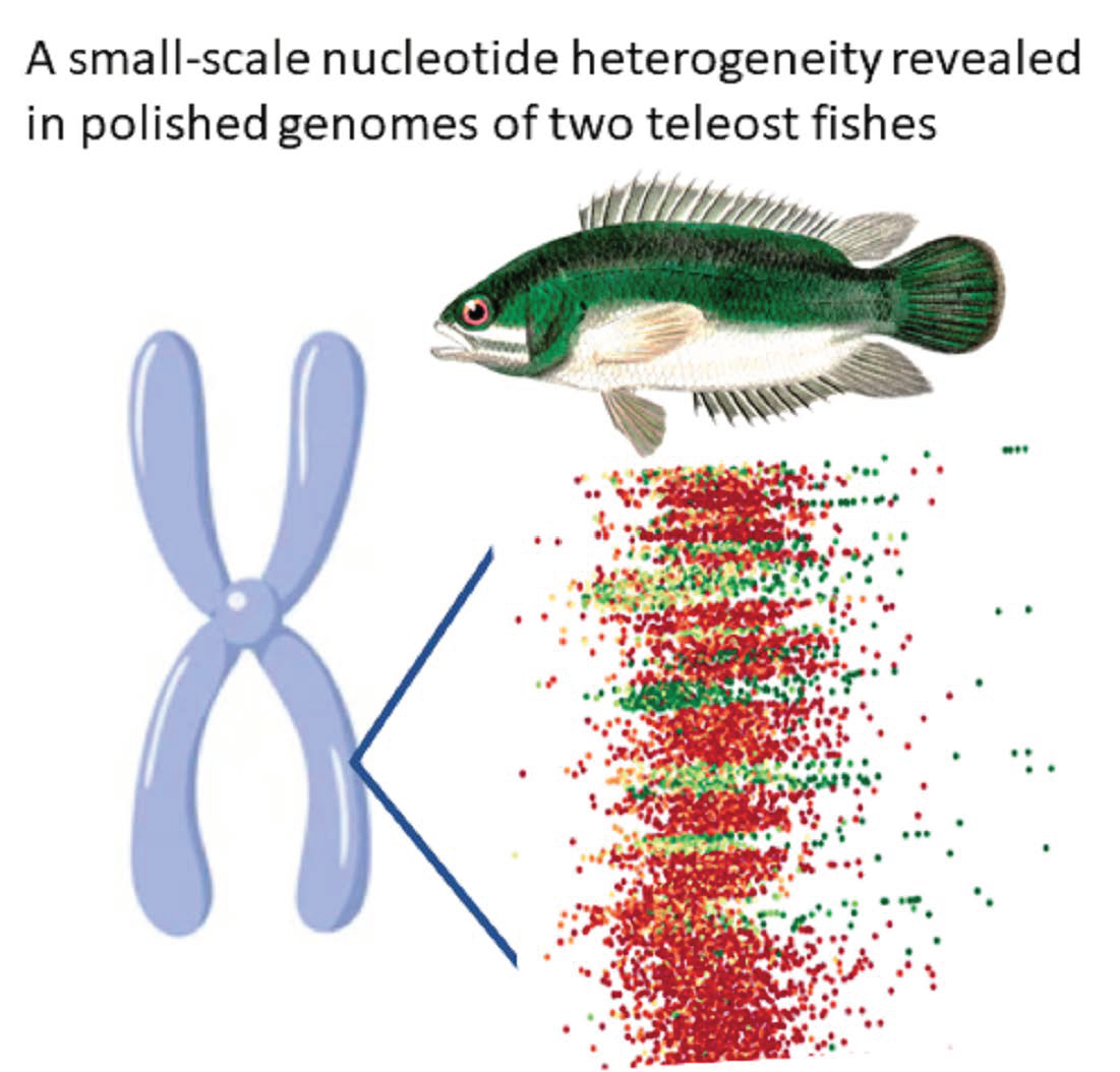
Hidden Compositional Heterogeneity of Fish Chromosomes in the Era of Polished Genome Assemblies

Abstract

Fish chromosomes are considered homogeneous in their AT/GC nucleotide composition, and banding patterns enabling identification of homologs are largely missing. While cytogenomic approaches try to compensate for this issue by virtual karyotyping, they rely on the quality of genome assemblies available. Recently, soft-masked genome assemblies combining costly and arduous long- and short-read sequencing and new generation assemblers became available for two teleost fish species, climbing perch (Anabas testudineus) and channel bull blenny (Cottoperca gobio). Soft-masking turns repetitive sequences in a genome assembly into lower case letters, leaving unique sequences in upper case. This enables investigators to assess the proportion of guanine and cytosine nucleotides (GC%) of transposable elements as an indicator of AT/GC homogenisation in fish. We have developed a new version of our Python tool Evan, which utilises chromosome-level genome assemblies and combines the profiles of GC% and the proportion of repeats (rep%) along chromosomes. Our profiles of both of those fishes showed clear and abrupt but small-scale fluctuations in GC% along otherwise compositionally homogenised sequences. Our study also highlights the key role of the sliding window size in determining the resolution of GC% profiling. While the quality of the genome assemblies appeared to be sufficient for GC%/rep% profiling, more effective repeat masking is necessary to better distinguish to what extent repeats compositionally homogenize fish genomes.

1. Introduction

Fish cytogenetics traditionally suffers from the lack of robust banding patterns [1] in numerous species, and is further hampered by the small sizes and high number of fish chromosomes [2]. This leads to difficulties with distinguishing pairs of homologous chromosomes [3,4,5]. While several attempts have been made to apply G-banding to fish cytogenetics, the results have been largely variable [6,7,8,9] and unsuccessful [8,10,11]. Consequently, to identify homologous pairs, BrdU-labelling to visualise the early and late-replication regions [12,13,14,15] has been applied to fish chromosomes, along with fluorescence in situ hybridisation (FISH) of restriction fragments [12,13,15,16] and ribosomal or bacterial artificial chromosome markers [17]. So far, the only successful application of G-banding to fish chromosomes (proved by bioinformatics) has been with the extant genera Lepisosteus and Atractosteus [18] of ancient ray-fin fishes gars. In the closest living relative of gars, the bowfin (Amia calva), G-banding does not produce any reproducible pattern [19]. Hence, understanding the reason for the lack of proper banding patterns and the development of ways to compensate for it still represent a challenge for fish cytogenetics and cytogenomics utilising genomics data. The missing banding patterns in fish has been ascribed to the AT/GC nucleotide composition [8], but the exact reasons and mechanisms behind it remain controversial [20]. Two mostly competing hypotheses have been put forward to explain the compositional difference between higher and lower vertebrates (and invertebrates): the (neo)selectionist hypothesis highlights a higher thermal resistance of GC-rich DNA and RNA [21], while the neutral hypothesis is based on GC-biased gene conversion [22]. However, since neither hypothesis is able to provide a satisfactory explanation, another approach that takes the proportion of guanine and cytosine nucleotides (GC%) of transposable elements (TEs) into consideration has been introduced [1,23]. This approach finds support in a recent study on the GC content of TEs [24]; however, further research is required to obtain more information on regional GC% of TEs in teleost and non-teleost fishes.

With the increasing availability of genomic data, the quantitative cytogenomics approach is gaining recognition since it offers a higher resolution and the possibility of quantifying chromosomal traits (regional and global GC% and repeats in soft-masked genomes), which is in contrast to traditional (molecular) cytogenetics. Quantitative cytogenomics opens up new possibilities in the characterisation of molecular traits along chromosomes, where large, cytogenetically detectable, alternating blocks of AT- and GC-rich regions are missing [25].

Here, we utilised the latest versions of two fish genome assemblies produced by the combination of long- and short-read sequencing technologies [26] to assess their potential in virtual karyotype analysis and visualisation over previous (single technology) sequencing approaches. Soft-masked versions of these high-quality genome assemblies are publicly available from the databases Ensembl [27] and NCBI [28].

Our tailored Python tool Evan 1.0 and the newly available genome assemblies revealed small-scale fluctuations in GC%, demonstrating the utility of combining high-quality genome assemblies with the detailed and careful profiling of GC% and the proportion of repeats (rep%). This study is the point of a long-term effort to elucidate the AT/GC compositional evolution across invertebrates and finally vertebrates, where so far, ununderstood differences exist between fishes (generally cold-blooded vertebrates) and higher (warm-blooded) vertebrates.

2. Materials and Methods

2.1. Code and Availability

Our tailored Python tool, Evan, performs the calculations and visualisation (i.e., profiling) of GC% and rep% along chromosomes. The tool is partly based on our previous code [1]. Evan is available on GitHub https://github.com/martavohnoutova/Evan (accessed on 27 November 2022) as a Jupyter notebook configured for the Linux operating system, where all analyses presented here can be repeated, the analyses of other species can be easily performed, and the large-scale profiles of GC% and rep% can be stored.

Evan requires the free data science platform ANACONDA www.anaconda.com (accessed on 27 November 2022) to simplify package management and deployment for Windows, Linux, and macOS. Evan further requires BioPython https://biopython.org (accessed on 27 November 2022), a set of freely available tools for biological computation written in Python. The workflow is described in detail and available in its entirety on the abovementioned GitHub link. The workflow includes the following steps:

1. Setting up of the Evan Python environment in bash/Linux (to be performed only once), finalisation by the activation of the Evan environment, and the starting of the dedicated Jupyter notebook prior to each session.

2. Installation (to be performed only once) of the following Python packages during the setup of the environment: scipy, matplotlib, csv, jupyter, pip, pandas, numpy, wget, gzip, and fpdf using conda (the package management system of ANACONDA).

3. Import of all packages has to be performed each time prior to working with Evan as with all other parts of this code.

4. Configuration of the Jupyter notebook (setting the working directory, setting the desired non-overlapping sliding window size by the number of nucleotides (nt; 1000 nt set as default), and defining the species to be analysed). This workflow assumes that genome assemblies to be profiled in the analysis are saved locally.

5. Scanning of the genome assembly with the above-defined non-overlapping sliding window collects data for an overview scatter plot of the mean GC% and rep% per chromosome.

6. Scatter plots of the mean GC% values for each chromosome from the above data are drawn. The following colour code is applied: reddish, unique sequences; greenish, repetitive sequences; yellow/orange, intermediate values of unique and repetitive sequences. The exact percentage of rep% is given at a provided scalebar that is tailored for each chart or chromosome in the case of profiles.

7. Data collection on the unmasked (non-repetitive; GC% of the upper case-labelled nts) and soft-masked (repetitive; gc% of the lower case-labelled nts) fractions. This is particularly useful for the quick determination of GC% in the repetitive fraction (i.e., gc%). A dictionary of GC%/gc% values is produced.

8. Profiles of GC% and rep% are plotted with the matplotlib library and saved together as a *.png image file. Depending on the window size, each 1000-nt sequence is represented by a dot with the colour reflecting rep%, as described above.

2.2. Genome Assemblies Used, Their History, and the Underlying Sequencing

The genome assembly fAnaTes1.2 (GCA_900324465.2) of the climbing perch (Anabas testudineus) was updated with Ensembl release 103 in February 2021 (www.ensembl.info/2021/02/15/ensembl-103-has-been-released/; accessed on 27 November 2022, the first Ensembl genome of this species was published in 2018 in release 94, together with 37 other fish species). The latest genome assembly was provided by the Wellcome Sanger Institute and Cambridge University (www.sanger.ac.uk/science/data/vertebrate-genomes-sequencing) Vertebrate Genomes Project (http://vertebrategenomesproject.org). Details on the sequencing technologies used are available on the website of the European Nucleotide Archive (ENA; www.ebi.ac.uk/ena/browser/view/GCA_900324465.2 for all links in this section accessed on 27 November 2022). Briefly, sequencing data for this assembly were produced by combining 68× coverage PacBio Sequel and 114× coverage Illumina HiSeqX data from a 10× Genomics Chromium library generated at the Wellcome Sanger Institute, BioNano Saphyr DLE data generated at the Rockefeller University Vertebrate Genome Laboratory, and 170× coverage HiSeqX data from a Hi-C library prepared by Arima Genomics [29].

The genome assembly fCotGob3.1 (GCA_900634415.1) of the channel bull blenny (Cottoperca gobio) was published in September 2019 with Ensembl release 98 (https://www.ensembl.info/2019/09/26/ensembl-98-has-been-released/). As above, the sequencing effort developed to produce this assembly is described in detail on the ENA website (https://www.ebi.ac.uk/ena/browser/view/GCA_900634415.1). The assembly for C. gobio was produced by combining the following: ~75× coverage PacBio Sequel data, ~54× coverage Illumina HiSeqX data generated from a 10× Genomics Chromium library obtained at the Wellcome Sanger Institute, BioNano Saphyr, two-enzyme data generated by BioNano, and ~145× coverage HiSeqX data from a Hi-C library prepared by Arima Genomics.

2.3. Soft-Masking of Genome Assemblies

Since the level of soft-masking of the genome assemblies in Ensembl was insufficient, we performed our own soft-masking to improve the quality of resulting profiles. We masked repeats using Dfam TE Tools container/v1.7 [29] and a library created by the tool RepeatModeler/v2.0.4 of de novo predictions for repeat masking by RepeatMasker/v4.1.4. The files produced by RepeatModeler (*.fna.ori.out) with masked positions in the genomes were further processed by BEDtools/v2.29.2 [30] with the maskfasta-soft setting, resulting in the final soft-masked genomes. The assemblies with additional masking and soft-masking in this study are labelled Anabas_OIST and Cottoperca_OIST.

3. Results

The mean GC% values of the whole chromosomes were 40–41% for both A. testudineus and C. gobio (Figure 1 ), with entire genome GC% values of 40.4% and 41%, respectively. The GC% values of the chromosomes were more tightly related to their size in C. gobio (R² = 0.6562) than in A. testudineus (R² = 0.2099), as shown in Figure 1. This reflects the relationship between the strength of recombination and GC%. The proportion of soft-masked sequences was low in the original assemblies (approximately 18% for C. gobio and 11.5% for A. testudineus). Hence, we performed our own repeat- and soft-masking (details in

Table 1. Summary of the species studied and their genome assemblies.

Trait/Species	Anabas testudineus	Cottoperca gobio
Order	Anabantiformes	Perciformes
Family	Anabantidae	Bovichtidae
Diploid chromosome number (2n)	46	48
Genome assembly size (Mb)	555.6	609.4
NCBI GC%	40.46%	41%
GC% calculated in this study	40.40%	40.96%
Proportion of soft-masked regions (orig.) 1	11.52%	18.15%
Proportion of soft-masked regions (new) 2	15.2%	25.01%
GC% of soft-masked/repetitive regions	38.40%	40.54%
GC% of unmasked/non-repetitive regions	40.66%	41.05%

¹ Soft-masking available for the genome assembly in Ensembl. ² Soft-masking performed in this study.

). The GC% of the soft-masked (i.e., repetitive) fractions were 38.4% for A. testudineus and 40.54% for C. gobio, showing that the repeat regions have a lower GC% than the entire genome and the unmasked fraction in A. testudineus. These three GC% values are comparable in C. gobio (summary for both species in Table 1).

Although dependent on the quality of soft-masking, the entire-chromosome repeat content (rep%; coloured according to the scale in Figure 2) provided valuable insight. Firstly, a putative sex chromosome (no. 18) in A. testudineus was identified by its high rep% value (Figure 2, green colour). Secondly, an increase in rep% values (more red/orange) was apparent with decreasing chromosome size in C. gobio, indicating a positive correlation between chromosome size and recombination rate (Figure 1).

In all chromosomes of C. gobio, small-scale fluctuations in regional GC% are visible (Figure 3). There are clear depletions in lower-GC% sequences in regions of elevated GC% as well as depletions in higher-GC% sequences in regions of decreased GC%. These changes in GC% form clear shifts in the GC% profile. The size of the peaks/troughs is approximately 200 kbp and mostly ranges between 100 and 300 kbp in C. gobio (estimated manually on zoomed in profiles).

In A. testudineus, the GC% fluctuations are even more pronounced (Figure 4). The size of the peaks/troughs is approximately 200 kbp and mostly ranges between 100 and 300 kbp. Despite the low efficiency of the repeat masking, repeats again occurred in regions with changes in GC% values, compensating for both regional increases and decreases (Figure 4). In other words, the few soft-masked sequences relatively blurred the small-scale changes in the profile of GC% values. Similar situations were seen for C. gobio (Figure 3 and online available profiles).

For both species, a higher range of the GC% values were apparent in the soft-masked sequences, particularly in telomeric regions. In the GC% profiling tool Evan, we created the sliding window with a different window size to visually prove, that the window size influences the visualization of GC% values spread—Figure 5. We were able to discover the most of GC% variance in the genomes with 1 kb window size.

Full-size profiles of all chromosomes of both species are available on our online GitHub repository (https://github.com/martavohnoutova/Evan). The figures in Appendix A, as with Figure A1 and Figure A2, show smaller versions of the virtual karyotypes of the species analysed here. Owing to the downscaling of the images for the purpose of publication, the images lack resolution, and fine details in the profiles cannot be seen. Therefore, we highly recommend that the full-size images on GitHub are viewed with the zoom function to fully take advantage of the profiles.

4. Discussion

This study demonstrated that a small, non-overlapping sliding window size of 1000 bp was able to yield GC% profiles with a sufficient resolution to identify hitherto hidden fluctuations in nucleotide composition in two teleost genomes. The standard window size is of 100,000 bp (100 kb) and is routinely used not only in mammals [31], but also in far smaller genomes of invertebrates [32]. However, this window size is unsuitable for fish genomes, which can be two to three times smaller. The chromosomes of both species profiled in this study showed small-scale patterns of alternating increases and decreases in GC%. Depending on the level of soft-masking, interstitial and telomeric regions of accumulated repeat were apparent and formed banding patterns. In general, the telomeric repeats showed a higher accumulation of repeats of diversified GC% values.

The GC%/rep% profiles for A. testudineus presented here are the first to be reported and hence cannot be compared with any previous version; the first assembled genome for species was not at the chromosome level. For C. gobio, a previous version of the profile has been produced, although it has not been published or explicitly mentioned in the literature [1]. The size of peaks/troughs in GC% values are smaller in these two fish species (and likely in other teleosts) than in mammals [1] and may explain why they are not detectable cytogenetically on chromosomes and why routine bioinformatic approaches utilising far larger sliding window sizes than here (1000 bp) cannot detect them in genome assemblies. It is also necessary to take into account that mammalian genomes are on average two to three times larger than those of teleost fish, meaning introns in fish genomes are also smaller than in mammals [33]. This could justify the need for the use of smaller sliding window size(s) for fish genomes. On the other hand, there are exceptions to this trend among teleosts; for instance, zebrafish show an unusual distribution of intron sizes, with a greater number of larger introns in general [34]. This may explain the exceptionally AT/GC homogenised genome in zebrafish [1], which was previously considered to be a typical teleost genome. Thus, the unusually AT-rich, TE-rich, and AT/GC homogenised zebrafish genome should not be considered a typical representative of teleost genomes. The extent of TEs and their GC% has to be considered when assessing the AT/GC homogeneity of fish genomes, together with the general diversity and speciosity of fishes.

Neither of the two fish species studied here are classified as typical model species. On the contrary, their chromosomes have not been characterised in as much detail as numerous others. For example, neither fish has been subjected to a routine localisation of rRNA genes [35,36,37,38]. Currently, for both species, 5S rRNA gene mapping to their genome assemblies has only been performed for unplaced scaffolds in Ensembl [27] using the online Ensembl tool BioMart (www.ensembl.org accessed on 27 November 2022). Hence, the current quality of assembled genomes is still insufficient to visualise the ribosomal genes that may provide a link between traditional cytogenetics and bioinformatics-based cytogenomics. However, even in the human genome, numerous ribosomal gene repeats have only been correctly assembled in the latest version, despite decades of effort [39]. A. testudineus is an example of a species in which we have a limited knowledge of its chromosomes [35,36,37] with largely unclear morphologies. Studies on A. testudineus have been largely focused on the differences between the various forms of the fish (spotted, non-spotted, native, introduced), and detailed knowledge of this species’ chromosomes may be retrieved from its genome assembly in the future. The chromosomes of C. gobio have been better characterised [40,41]; however, the fact that all of them are acrocentric, with centromeres located towards one end of each chromosome, makes identification of their homologous pairs challenging. On the other hand, their acrocentric morphology simplifies their interpretation since no internal centromeric repetitive regions exist, as in submetacentric and metacentric chromosomes. This means that any internal accumulations of repetitive sequences can be ascribed to structures other than the centromeres. The accumulation of internal repeat in the form of green bands (i.e., the highest proportion of soft-masking) is clearly apparent in chromosomes LR131934 and LR131938 in Figure A1. In chromosomes LR191335, −39, −31, −25, and −21, there are also interstitial regions where only AT nucleotides occur, resulting in drops in GC% to zero. These regions, however, lack any soft-masking (red dots).

Besides the primary usage in GC% profiling along chromosomes, Evan also proved to be particularly useful for the quick determination of the quality and efficiency of soft-masking. Since Evan directly displays repetitive fractions along chromosome sequences on a colour scale, the efficiency of soft-masking can be assessed. However, the quality of soft-masking also determines how informative the output values of Evan are. In general, fish genomes are known to contain a high proportion of repeats (20–40%) [42,43]. The highest proportions of repeats have been recorded in cyprinid and salmonid fishes, reaching up to 60% [43,44]. The lowest repeat proportions of around 10% are known in the compact and well-assembled genomes of tetraodontiform fishes [43]. The true amount of repeats of C. gobio and A. testudineus is probably higher than the percentage of repeats masked in this study (15 and 25%). The insufficient quality of repeat masking libraries still persists as one of the limiting factors in identifying the GC% content of repeats. As we have shown in this study, it is necessary to combine more tools to identify repeats and, as many as possible, repeat libraries. Although the only really complete genome assembly is the latest version of the human genome, T2T-CHM13 [39], there are other technologies available for non-model species. For example, Hi-C has been applied to the black rockfish (Sebastes schlegelii) [45]. The Hi-C technology enables more precise ordering and orienting of sequences into scaffolds, after which assembly errors can be identified and corrected, and better chromosome-level genome assemblies can be produced [46]. Thus, our study represents the first steps in utilising all possible technologies towards understanding the genome composition in teleost and non-teleost fishes.

5. Conclusions

The newly available genome assemblies are a highly promising resource for our understanding of the compositional organisation of fish chromosome-level DNA sequences. Each run of repeat masking with newly available libraries of repeats improves the profiles and increases their resolution. A small sliding window (1000 bp) is also crucial since it is more appropriate for the smaller genome and chromosome sizes in fish genomes.

References

1. Matoulek, D.; Borůvková, V.; Ocalewicz, K.; Symonová, R. GC and Repeats Profiling along Chromosomes—The Future of Fish Compositional Cytogenomics. Genes 2020, 12, 50. [Google Scholar] [CrossRef] [PubMed]
2. Borůvková, V.; Howell, W.M.; Matoulek, D.; Symonová, R. Quantitative Approach to Fish Cytogenetics in the Context of Vertebrate Genome Evolution. Genes 2021, 12, 312. [Google Scholar] [CrossRef]
3. Knytl, M.; Kalous, L.; Rab, P. Karyotype and Chromosome Banding of Endangered Crucian Carp, Carassius Carassius (Linnaeus, 1758) (Teleostei, Cyprinidae). CCG 2013, 7, 205–213. [Google Scholar] [CrossRef]
4. Knytl, M.; Kalous, L.; Symonová, R.; Rylková, K.; Ráb, P. Chromosome Studies of European Cyprinid Fishes: Cross-Species Painting Reveals Natural Allotetraploid Origin of a Carassius Female with 206 Chromosomes. Cytogenet. Genome Res. 2013, 139, 276–283. [Google Scholar] [CrossRef] [PubMed]
5. Knytl, M.; Fornaini, N. Measurement of Chromosomal Arms and FISH Reveal Complex Genome Architecture and Standardized Karyotype of Model Fish, Genus Carassius. Cells 2021, 10, 2343. [Google Scholar] [CrossRef]
6. Bertollo, L.A.C.; Fontes, M.S.; Fenocchio, A.S.; Cano, J. The X1X2Y Sex Chromosome System in the Fish Hoplias Malabaricus. I. G-, C- and Chromosome Replication Banding. Chromosome Res. 1997, 5, 493–499. [Google Scholar] [CrossRef]
7. Gold, J.R.; Li, Y.C. Trypsin G-Banding of North American Cyprinid Chromosomes: Phylogenetic Considerations, Implications for Fish Chromosome Structure, and Chromosomal Polymorphism. Cytologia 1991, 56, 199–208. [Google Scholar] [CrossRef]
8. Medrano, L.; Bernardi, G.; Couturier, J.; Dutrillaux, B.; Bernardi, G. Chromosome Banding and Genome Compartmentalization in Fishes. Chromosoma 1988, 96, 178–183. [Google Scholar] [CrossRef]
9. Wiberg, U.H. Sex Determination in the European Eel (Anguilla Anguilla, L.). Cytogenet. Genome Res. 1983, 36, 589–598. [Google Scholar] [CrossRef]
10. Luo, C. Multiple Chromosomal Banding in Grass Carp, Ctenopharyngodon Idellus. Heredity 1998, 81, 481–485. [Google Scholar] [CrossRef]
11. Swarça, A.C.; Fenocchio, A.S.; Cestari, M.M.; Dias, A.L. First Chromosome Data on Steindachneridion Scripta (Pisces, Siluriformes, Pimelodidae) from Brazilian Rivers: Giemsa, CBG, G-, and RE Banding. Genet. Mol. Res. 2005, 4, 734–741. [Google Scholar] [PubMed]
12. Jankun, M.; Mochol, M.; Ocalewicz, K. Conventional and Molecular Cytogenetics of the Pikeperch (Sander Lucioperca L.). Aquac. Res. 2014, 45, 1084–1089. [Google Scholar] [CrossRef]
13. Jankun, M.; Ocalewicz, K.; Mochol, M. Chromosome Banding Studies by Replication and Restriction Enzyme Treatment in Vendace (Coregonus Albula) (Salmonidae, Salmoniformes). Folia Biol Krakow 2004, 52, 47–51. [Google Scholar]
14. Jankun, M.; Ocalewicz, K.; Woznicki, P. Replication, C- and Fluorescent Chromosome Banding Patterns in European Whitefish, Coregonus Lavavetus L. Hereditas 2004, 128, 195–199. [Google Scholar] [CrossRef]
15. de Araújo, W.C.; Martínez, P.A.; Molina, W.F. Mapping of Ribosomal DNA by FISH, EcoRI Digestion and Replication Bands in the Cardinalfish Apogon Americanus (Perciformes). Cytologia 2010, 75, 109–117. [Google Scholar] [CrossRef]
16. Viñas, A.; Gómez, C.; Martínez, P.; Sánchez, L. Induction of G-Bands on Anguilla Anguilla Chromosomes by the Restriction Endonucleases HaeLll, HinfI, and MseI. Cytogenet. Genome Res. 1994, 65, 79–81. [Google Scholar] [CrossRef] [PubMed]
17. Symonová, R.; Havelka, M.; Amemiya, C.T.; Howell, W.M.; Kořínková, T.; Flajšhans, M.; Gela, D.; Ráb, P. Molecular Cytogenetic Differentiation of Paralogs of Hox Paralogs in Duplicated and Re-Diploidized Genome of the North American Paddlefish (Polyodon Spathula). BMC Genet. 2017, 18, 19. [Google Scholar] [CrossRef]
18. Symonová, R.; Majtánová, Z.; Arias-Rodriguez, L.; Mořkovský, L.; Kořínková, T.; Cavin, L.; Pokorná, M.J.; Doležálková, M.; Flajšhans, M.; Normandeau, E.; et al. Genome Compositional Organization in Gars Shows More Similarities to Mammals than to Other Ray-Finned Fish. J. Exp. Zool. (Mol. Dev. Evol.) 2017, 328, 607–619. [Google Scholar] [CrossRef]
19. Majtánová, Z.; Symonová, R.; Arias-Rodriguez, L.; Sallan, L.; Ráb, P. “Holostei versus Halecostomi” Problem: Insight from Cytogenetics of Ancient Nonteleost Actinopterygian Fish, Bowfin Amia Calva. J. Exp. Zool. (Mol. Dev. Evol.) 2017, 328, 620–628. [Google Scholar] [CrossRef]
20. Matoulek, D.; Ježek, B.; Vohnoutová, M.; Symonová, R. Advances in Vertebrate (Cyto)Genomics Shed New Light on Fish Compositional Genome Evolution. Genes 2023, 14, 244. [Google Scholar] [CrossRef]
21. Bernardi, G. The Neoselectionist Theory of Genome Evolution. Proc. Natl. Acad. Sci. USA 2007, 104, 8385–8390. [Google Scholar] [CrossRef] [PubMed]
22. Galtier, N. Fine-Scale Quantification of GC-Biased Gene Conversion Intensity in Mammals. Peer Community J. 2021, 1, e17. [Google Scholar] [CrossRef]
23. Symonová, R.; Suh, A. Nucleotide Composition of Transposable Elements Likely Contributes to AT/GC Compositional Homogeneity of Teleost Fish Genomes. Mobile DNA 2019, 10, 49. [Google Scholar] [CrossRef] [PubMed]
24. Boissinot, S. On the Base Composition of Transposable Elements. Int. J. Mol. Sci. 2022, 23, 4755. [Google Scholar] [CrossRef]
25. Gaffaroglu, M.; Majtánová, Z.; Symonová, R.; Pelikánová, Š.; Unal, S.; Lajbner, Z.; Ráb, P. Present and Future Salmonid Cytogenetics. Genes 2020, 11, 1462. [Google Scholar] [CrossRef]
26. Rhie, A.; McCarthy, S.A.; Fedrigo, O.; Damas, J.; Formenti, G.; Koren, S.; Uliano-Silva, M.; Chow, W.; Fungtammasan, A.; Kim, J.; et al. Towards Complete and Error-Free Genome Assemblies of All Vertebrate Species. Nature 2021, 592, 737–746. [Google Scholar] [CrossRef]
27. Cunningham, F.; Allen, J.E.; Allen, J.; Alvarez-Jarreta, J.; Amode, M.R.; Armean, I.M.; Austine-Orimoloye, O.; Azov, A.G.; Barnes, I.; Bennett, R.; et al. Ensembl 2022. Nucleic Acids Res. 2022, 50, D988–D995. [Google Scholar] [CrossRef]
28. National Library of Medicine (US). National Center for Biotechnology Information (NCBI) [Internet]. Bethesda (MD): National Library of Medicine (US), National Center for Biotechnology Information. 1998. Available online: https://www.ncbi.nlm.nih.gov/ (accessed on 28 March 2023).
29. Flynn, J.M.; Hubley, R.; Goubert, C.; Rosen, J.; Clark, A.G.; Feschotte, C.; Smit, A.F. RepeatModeler2 for Automated Genomic Discovery of Transposable Element Families. Proc. Natl. Acad. Sci. USA 2020, 117, 9451–9457. [Google Scholar] [CrossRef]
30. Quinlan, A.R.; Hall, I.M. BEDTools: A Flexible Suite of Utilities for Comparing Genomic Features. Bioinformatics 2010, 26, 841–842. [Google Scholar] [CrossRef]
31. Cozzi, P.; Milanesi, L.; Bernardi, G. Segmenting the Human Genome into Isochores. Evol. Bioinform. 2015, 11, EBO-S27693. [Google Scholar] [CrossRef]
32. Lamolle, G.; Protasio, A.V.; Iriarte, A.; Jara, E.; Simón, D.; Musto, H. An Isochore-Like Structure in the Genome of the Flatworm Schistosoma Mansoni. Genome Biol. Evol. 2016, 8, 2312–2318. [Google Scholar] [CrossRef]
33. Jakt, L.M.; Dubin, A.; Johansen, S.D. Intron Size Minimisation in Teleosts. BMC Genom. 2022, 23, 628. [Google Scholar] [CrossRef] [PubMed]
34. Moss, S.P.; Joyce, D.A.; Humphries, S.; Tindall, K.J.; Lunt, D.H. Comparative Analysis of Teleost Genome Sequences Reveals an Ancient Intron Size Expansion in the Zebrafish Lineage. Genome Biol. Evol. 2011, 3, 1187–1196. [Google Scholar] [CrossRef] [PubMed]
35. Mazzei, F.; Ghigliotti, L.; Lecointre, G.; Ozouf-Costaz, C.; Coutanceau, J.-P.; Detrich, W.; Pisano, E. Karyotypes of Basal Lineages in Notothenioid Fishes: The Genus Bovichtus. Polar Biol. 2006, 29, 1071. [Google Scholar] [CrossRef]
36. Kabir, M.A.; Habib, M.A.; Hasan, M.; Alam, S.S. Genetic Diversity in Three Forms of Anabas Testudineus Bloch. Cytologia 2012, 77, 231–237. [Google Scholar] [CrossRef]
37. Khuda-Bukhsh, A.R.; Chakrabarti, C. Differential C-Heterochromatin Distribution in Two Species of Freshwater Fish, Anabas Testudineus (Bloch.) and Puntius Sarana (Hamilton.). Indian J. Exp. Biol. 2000, 38, 265–268. [Google Scholar]
38. Tinni, S.R.; Jessy, N.S.; Hasan, M.M.; Mustafa, M.G.; Alam, S.S. Comparative Karyotype Analysis with Differential Staining in Two Forms of Anabas Testudineus Bloch. Cytologia 2007, 72, 71–75. [Google Scholar] [CrossRef]
39. Nurk, S.; Koren, S.; Rhie, A.; Rautiainen, M.; Bzikadze, A.V.; Mikheenko, A.; Vollger, M.R.; Altemose, N.; Uralsky, L.; Gershman, A.; et al. The Complete Sequence of a Human Genome. Science 2022, 376, 44–53. [Google Scholar] [CrossRef]
40. Pisano, E.; Ozouf-Costaz, C.; Hureau, J.-C.; Williams, R. Chromosome Differentiation in the Subantarctic Bovichtidae Species Cottoperca Gobio (Günther, 1861) and Pseudaphritis Urvillii (Valenciennes, 1832) (Pisces, Perciformes). Antart. Sci. 1995, 7, 381–386. [Google Scholar] [CrossRef]
41. Pisano, E.; Ozouf-Costaz, C. Chromosome Change and the Evolution in the Antarctic Fish Suborder Notothenioidei. Antart. Sci. 2000, 12, 334–342. [Google Scholar] [CrossRef]
42. Canapa, A.; Barucca, M.; Biscotti, M.A.; Forconi, M.; Olmo, E. Transposons, Genome Size, and Evolutionary Insights in Animals. Cytogenet. Genome Res. 2015, 147, 217–239. [Google Scholar] [CrossRef] [PubMed]
43. Yuan, Z.; Liu, S.; Zhou, T.; Tian, C.; Bao, L.; Dunham, R.; Liu, Z. Comparative Genome Analysis of 52 Fish Species Suggests Differential Associations of Repetitive Elements with Their Living Aquatic Environments. BMC Genom. 2018, 19, 141. [Google Scholar] [CrossRef] [PubMed]
44. Lien, S.; Koop, B.F.; Sandve, S.R.; Miller, J.R.; Kent, M.P.; Nome, T.; Hvidsten, T.R.; Leong, J.S.; Minkley, D.R.; Zimin, A.; et al. The Atlantic Salmon Genome Provides Insights into Rediploidization. Nature 2016, 533, 200–205. [Google Scholar] [CrossRef] [PubMed]
45. Liu, Q.; Wang, X.; Xiao, Y.; Zhao, H.; Xu, S.; Wang, Y.; Wu, L.; Zhou, L.; Du, T.; Lv, X.; et al. Sequencing of the Black Rockfish Chromosomal Genome Provides Insight into Sperm Storage in the Female Ovary. DNA Res. 2019, 26, 453–464. [Google Scholar] [CrossRef]
46. Dudchenko, O.; Batra, S.S.; Omer, A.D.; Nyquist, S.K.; Hoeger, M.; Durand, N.C.; Shamim, M.S.; Machol, I.; Lander, E.S.; Aiden, A.P.; et al. De Novo Assembly of the Aedes Aegypti Genome Using Hi-C Yields Chromosome-Length Scaffolds. Science 2017, 356, 92–95. [Google Scholar] [CrossRef] [PubMed]
Figure 1. Relationships between the GC% and corresponding chromosome size in Anabas testudineus (left) and Cottoperca gobio (right) on equidistant axes.
Fishes 08 00185 g001
Figure 2. Overview of the two genome assemblies analysed in this study. Each chromosome (x-axis) is represented as a dot, with the y-axis showing GC% values. Chromosomes are sorted by size, from largest to smallest. The colour gradients of the dots reflect the proportion of soft-masked sequences (rep%) with the two extremes being red, indicating unmasked, and green, indicating soft-masked regions. The colour scale below each graph represents a species-specific flexible range of the soft-masking percentage. The sliding window size is 1000 nt for both species. A putative sex chromosome (no. 18) in A. testudineus is shown demonstrating a high proportion of repeats for its size.
Fishes 08 00185 g002
Figure 3. GC% profile of chromosome 22 in C. gobio (or LR131930 in ENA). x-axis, sequences in base pairs (bp); y-axis, GC%. The sliding window size is 1000 bp. Yellow arrows mark several selected decreases in GC%, forming drops in the profile, and blue arrows mark “protrusions” towards lower GC% values corresponding to the drops. Similarly, increases in GC% (e.g., between the labelled drops) are accompanied by shifts towards higher GC% values.
Fishes 08 00185 g003
Figure 4. GC% profile of chromosome 21 in A. testudineus (or LR13257 in ENA), showing clear fluctuations in GC% between ~30–50%. x-axis, sequences in base pairs (bp); y-axis, GC%. Regions with green dots are accumulations of repetitive (i.e., soft-masked) sequences. The sliding window size is 1000 bp.
Fishes 08 00185 g004
Figure 5. Distribution of GC% values resulting from the usage of five different sliding window sizes. Histograms for the two species, A. testudineus (left) and C. gobio (right), show a comparable reduction in the range of GC% values with increasing sliding window size. Note: For the histogram of GC% with the 100 kb sliding window size, which is routinely used in assessing the GC content of genomes, the bars are too small to be viewed at the scale of the image.
Fishes 08 00185 g005