
Environmental Characteristics Associated with the Presence of the Pelagic Stingray (Pteroplatytrygon violacea) in the Pacific High Sea


 and
and
Abstract
1. Introduction
2. Materials and Methods
2.1. Study Areas
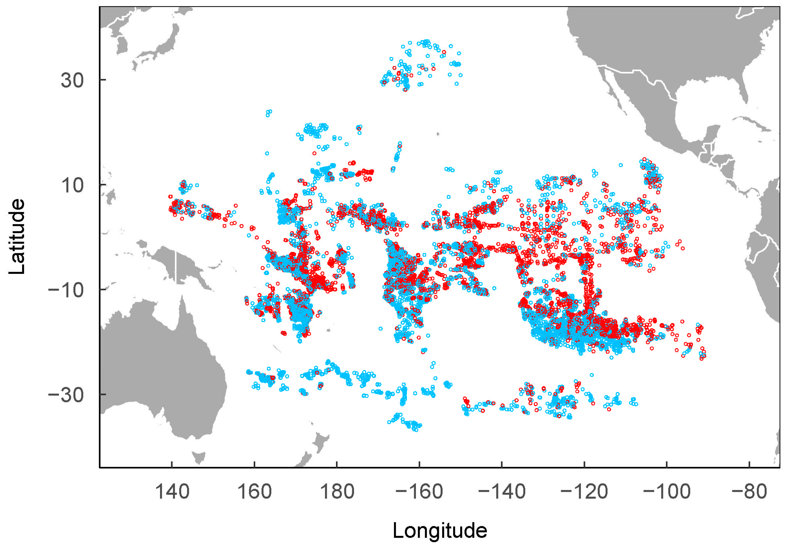
2.2. P. violacea Data
2.3. Environmental Data
2.4. Statistical Analysis
3. Results
4. Discussion
4.1. Environmental Preference of P. violacea
4.2. Impact of ENSO on the Presence of P. violacea in the Pacific High Sea
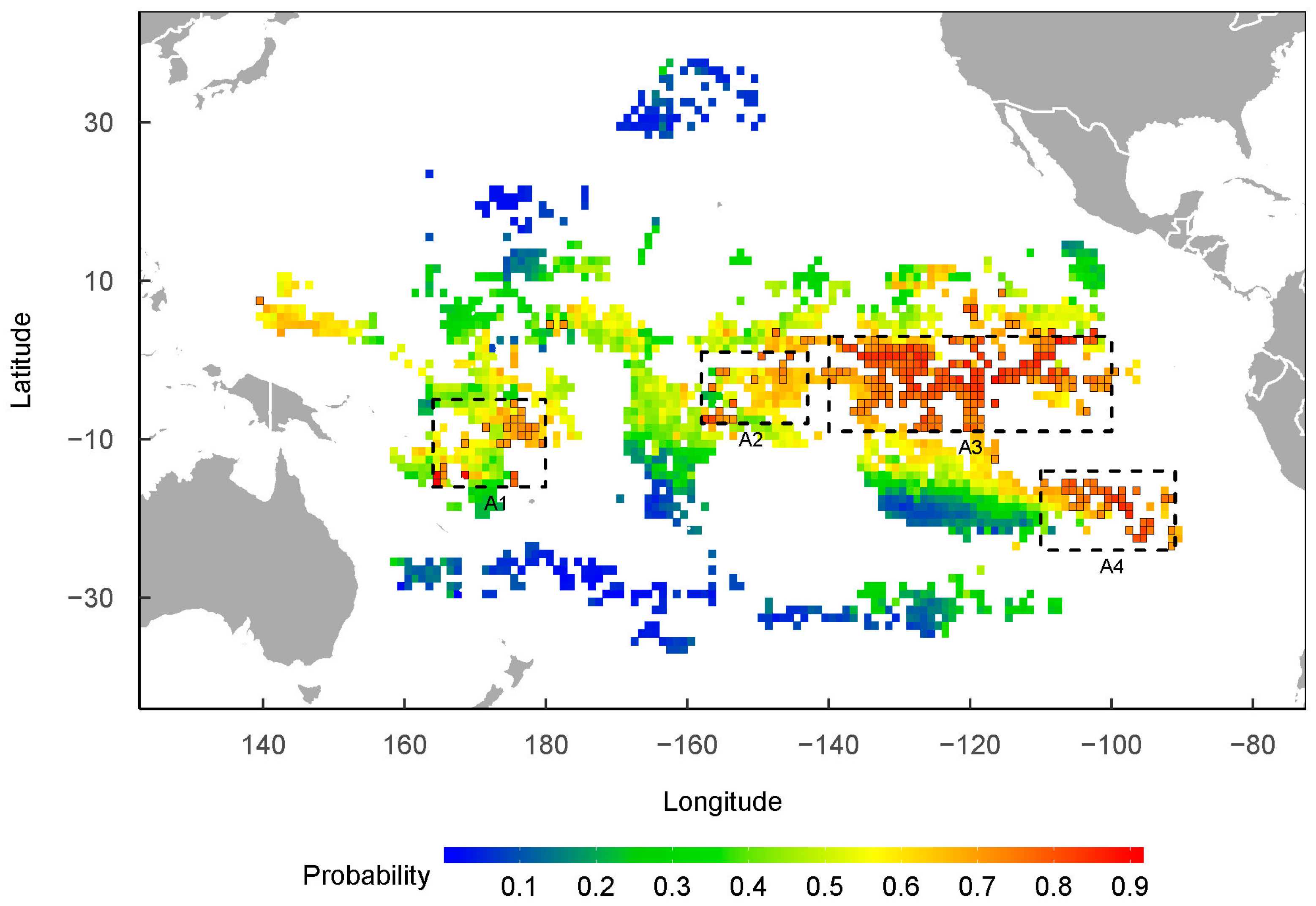
4.3. Spatial–Temporal Distribution of P. violacea in the Pacific High Sea
4.4. Conservation Consideration
5. Conclusions
Supplementary Materials
Author Contributions
Funding
Institutional Review Board Statement
Informed Consent Statement
Data Availability Statement
Acknowledgments
Conflicts of Interest
References
- Hall, M.; Alverson, D.; Metuzals, K. By-Catch: Problems and Solutions. Mar. Pollut. Bull. 2000, 41, 204–219. [Google Scholar] [CrossRef]
- Wang, J.; Gao, X.; Xu, L.; Dai, L.; Chen, J.; Tian, S.; Chen, Y. Biodiversity in the Bycatch Community of Chinese Tuna Longline Fisheries in the Pacific Ocean. Glob. Ecol. Conserv. 2020, 24, e01276. [Google Scholar] [CrossRef]
- FAO. International Plan of Action for the Conservation and Management of Sharks; FAO: Rome, Italy, 1999. [Google Scholar]
- FAO. International Plan of Action for Reducing Incidental Catch of Seabirds in Longline Fisheries; FAO: Rome, Italy, 1999. [Google Scholar]
- FAO. Guidelines to Reduce Sea Turtle Mortality in Fishing Operations; FAO: Rome, Italy, 2009. [Google Scholar]
- Clarke, S.; Sato, M.; Small, C.; Sullivan, B.; Inoue, Y.; Ochi, D. Bycatch in Longline Fisheries for Tuna and Tuna-like Species: A Global Review of Status and Mitigation Measures. FAO Fish. Aquac. Tech. Pap. 2014, 588, 1–199. [Google Scholar]
- Hilborn, R.; Agostini, V.N.; Chaloupka, M.; Garcia, S.M.; Gerber, L.R.; Gilman, E.; Hanich, Q.; Himes-Cornell, A.; Hobday, A.J.; Itano, D.; et al. Area-Based Management of Blue Water Fisheries: Current Knowledge and Research Needs. Fish Fish. 2021, 1–27. [Google Scholar] [CrossRef]
- Schlaff, A.M.; Heupel, M.R.; Simpfendorfer, C.A. Influence of Environmental Factors on Shark and Ray Movement, Behaviour and Habitat Use: A Review. Rev. Fish Biol. Fish. 2014, 24, 1089–1103. [Google Scholar] [CrossRef]
- Neer, J.A. The Biology and Ecology of the Pelagic Stingray, Pteroplatytrygon Violacea (Bonaparte, 1832). Sharks Open Ocean Biol. Fish. Conserv. 2009, 152–159. [Google Scholar] [CrossRef]
- Báez, J.C.; Crespo, G.O.; García-Barcelona, S.; De Urbina, J.M.O.; Macías, D. Understanding Pelagic Stingray (Pteroplatytrygon Violacea) by-Catch by Spanish Longliners in the Mediterranean Sea. J. Mar. Biol. Assoc. U. K. 2016, 96, 1387–1394. [Google Scholar] [CrossRef]
- Hare, S.R.; Williams, P.G.; Castillo Jordán, C.D.; Hamer, P.A.; Scott, R.D.; Pilling, G. The Western and Central Pacific Tuna Fishery: 2020 Overview and Status of Stocks; Pacific Community: Noumea, NC, USA, 2021; ISBN 9789820014206. [Google Scholar]
- Wang, J.; Gao, C.; Wu, F.; Gao, X.; Chen, J.; Dai, X.; Tian, S.; Chen, Y. The Discards and Bycatch of Chinese Tuna Longline Fleets in the Pacific Ocean from 2010 to 2018. Biol. Conserv. 2021, 255, 109011. [Google Scholar] [CrossRef]
- Ward, P.; Myers, R.A. Shifts in Open-ocean Fish Communities Coinciding with the Commencement of Commercial Fishing. Ecology 2005, 86, 835–847. [Google Scholar] [CrossRef]
- Polovina, J.J.; Woodworth-Jefcoats, P.A. Fishery-Induced Changes in the Subtropical Pacific Pelagic Ecosystem Size Structure: Observations and Theory. PLoS ONE 2013, 8, e62341. [Google Scholar] [CrossRef]
- Kirby, D.S.; Hobday, A. Ecological Risk Assessment for the Effects of Fishing in the Western and Central Pacific Ocean: Productivity-Susceptibility Analysis. In Proceedings of the WCPFC-SC3-EB-SWG/WP-1.Third Scientific Committee Meeting of the Western and Central Pacific Fisheries Commission, Honolulu, HI, USA, 13–24 August 2007. [Google Scholar]
- Lin, Q.; Chen, Y.; Zhu, J. A Comparative Analysis of the Ecological Impacts of Chinese Tuna Longline Fishery on the Eastern Pacific Ocean. Ecol. Indic. 2022, 143, 109284. [Google Scholar] [CrossRef]
- Kindong, R.; Sarr, O.; Wang, J.; Xia, M.; Wu, F.; Dai, L.; Tian, S.; Dai, X. Size Distribution Patterns of Silky Shark Carcharhinus Falciformis Shaped by Environmental Factors in the Pacific Ocean. Sci. Total Environ. 2022, 850, 157927. [Google Scholar] [CrossRef] [PubMed]
- Gilman, E.; Passfield, K.; Nakamura, K. Performance of Regional Fisheries Management Organizations: Ecosystem-Based Governance of Bycatch and Discards. Fish Fish. 2014, 15, 327–351. [Google Scholar] [CrossRef]
- Gilman, E.; Weijerman, M.; Suuronen, P. Ecological Data from Observer Programmes Underpin Ecosystem-Based Fisheries Management. ICES J. Mar. Sci. 2017, 74, 1481–1495. [Google Scholar] [CrossRef]
- Diaz-Delgado, E.; Crespo-Neto, O.; Martínez-Rincón, R.O. Environmental Preferences of Sharks Bycaught by the Tuna Purse-Seine Fishery in the Eastern Pacific Ocean. Fish. Res. 2021, 243, 106076. [Google Scholar] [CrossRef]
- Lopetegui-Eguren, L.; Poos, J.J.; Arrizabalaga, H.; Guirhem, G.L.; Murua, H.; Lezama-Ochoa, N.; Griffiths, S.P.; Gondra, J.R.; Sabarros, P.S.; Báez, J.C.; et al. Spatio-Temporal Distribution of Juvenile Oceanic Whitetip Shark Incidental Catch in the Western Indian Ocean. Front. Mar. Sci. 2022, 9, 1–19. [Google Scholar] [CrossRef]
- Lezama-Ochoa, N.; Hall, M.A.; Pennino, M.G.; Stewart, J.D.; López, J.; Murua, H. Environmental Characteristics Associated with the Presence of the Spinetail Devil Ray (Mobula Mobular) in the Eastern Tropical Pacific. PLoS ONE 2019, 14, 854. [Google Scholar] [CrossRef]
- Lopez, J.; Alvarez-Berastegui, D.; Soto, M.; Murua, H. Using Fisheries Data to Model the Oceanic Habitats of Juvenile Silky Shark (Carcharhinus Falciformis) in the Tropical Eastern Atlantic Ocean. Biodivers. Conserv. 2020, 29, 2377–2397. [Google Scholar] [CrossRef]
- Vilmar, M.; Di Santo, V. Swimming Performance of Sharks and Rays under Climate Change. Rev. Fish Biol. Fish. 2022, 32, 765–781. [Google Scholar] [CrossRef]
- Mollet, H.F. Distribution of the Pelagic Stingray, Dasyatis Violacea (Bonaparte, 1832), off California, Central America, and Worldwide. Mar. Freshw. Res. 2002, 53, 525–530. [Google Scholar] [CrossRef]
- Mollet, H.F.; Ezcurra, J.M.; O’Sullivan, J.B. Captive Biology of the Pelagic Stingray, Dasyatis Violacea (Bonaparte, 1832). Mar. Freshw. Res. 2002, 53, 531–541. [Google Scholar] [CrossRef]
- Williams, P.; Ruaia, T. Overview of Tuna Fisheries in the Western and Central Pacific Ocean, Including Economic Conditions-2019. In Proceedings of the WCPFC-SC16-2020/GN-IP-1. Sixteenth Regular Session of the WCPFC Scientific Committee, Online Meeting, 11–22 August 2020. [Google Scholar]
- Dai, X.; Wu, F.; Wang, X. Annual Report to the Commission Part 1: Information on Fisheries, Research and Statistics. In Proceedings of the WCPFC-SC15-AR/CCM–03, Fifteenth Regular Session of the WCPFC Scientific Committee, Pohnpei, Micronesia, 12–20 August 2019. [Google Scholar]
- Morato, T.; Hoyle, S.D.; Allain, V.; Nicol, S.J. Seamounts Are Hotspots of Pelagic Biodiversity in the Open Ocean. Proc. Natl. Acad. Sci. USA 2010, 107, 9707–9711. [Google Scholar] [CrossRef] [PubMed]
- Yesson, C.; Clark, M.R.; Taylor, M.L.; Rogers, A.D. The Global Distribution of Seamounts Based on 30 Arc Seconds Bathymetry Data. Deep Sea Res. Part I Oceanogr. Res. Pap. 2011, 58, 442–453. [Google Scholar] [CrossRef]
- Morato, T.; Varkey, D.A.; Damaso, C.; Machete, M.; Santos, M.; Prieto, R.; Santos, R.S.; Pitcher, T.J. Evidence of a Seamount Effect on Aggregating Visitors. Mar. Ecol. Prog. Ser. 2008, 357, 23–32. [Google Scholar] [CrossRef]
- Guisan, A.; Edwards Jr, T.C.; Hastie, T. Generalized Linear and Generalized Additive Models in Studies of Species Distributions: Setting the Scene. Ecol. Modell. 2002, 157, 89–100. [Google Scholar] [CrossRef]
- Wood, S.N. Generalized Additive Models: An Introduction with R; Chapman and Hall/CRC: London, UK, 2006; ISBN 0429093152. [Google Scholar]
- Akaike, H. A New Look at the Statistical Model Identification. IEEE Trans. Autom. Control 1974, 19, 716–723. [Google Scholar] [CrossRef]
- Fielding, A.H.; Bell, J.F. A Review of Methods for the Assessment of Prediction Errors in Conservation Presence/Absence Models. Environ. Conserv. 1997, 24, 38–49. [Google Scholar] [CrossRef]
- R Core Team. R Development Core Team. R A Lang. Environ. Stat. Comput. 2013, 55, 275–286. [Google Scholar]
- Wood, S.; Wood, M.S. Package ‘Mgcv’. R Packag. Version 2015, 1, 729. [Google Scholar]
- Team, R.C.; Team, M.R.C.; Suggests, M.; Matrix, S. Package Stats. R Stats Packag. 2018, 1–489. [Google Scholar]
- Wei, T.; Simko, V.; Levy, M.; Xie, Y.; Jin, Y.; Zemla, J. Package ‘Corrplot’. Statistician 2017, 56, e24. [Google Scholar]
- Fox, J.; Weisberg, S.; Adler, D.; Bates, D.; Baud-Bovy, G.; Ellison, S.; Firth, D.; Friendly, M.; Gorjanc, G.; Graves, S. Package ‘Car’. Vienna R Found. Stat. Comput. 2012, 16, 1–158. [Google Scholar]
- Freeman, E.A.; Moisen, G. PresenceAbsence: An R Package for Presence Absence Analysis. J. Stat. Softw. 2008, 23, 1–31. [Google Scholar] [CrossRef]
- Kuhn, M. Building Predictive Models in R Using the Caret Package. J. Stat. Softw. 2008, 28, 1–26. [Google Scholar] [CrossRef]
- Bernal, D.; Carlson, J.K.; Goldman, K.J.; Lowe, C.G. Energetics, Metabolism, and Endothermy in Sharks and Rays. Biol. Sharks Relat. 2012, 211, 237. [Google Scholar]
- Talley, L.D. Salinity Patterns in the Ocean. Earth Syst. Phys. Chem. Dimens. Glob. Environ. Chang. 2002, 1, 629–640. [Google Scholar]
- Musyl, M.K.; Brill, R.W.; Curran, D.S.; Fragoso, N.M.; McNaughton, L.M.; Nielsen, A.; Kikkawa, B.S.; Moyes, C.D. Postrelease Survival, Vertical and Horizontal Movements, and Thermal Habitats of Five Species of Pelagic Sharks in the Central Pacific Ocean. Fish. Bull. 2011, 109, 341–368. [Google Scholar]
- Lezama-Ochoa, N.; Murua, H.; Hall, M.; Román, M.; Ruiz, J.; Vogel, N.; Caballero, A.; Sancristobal, I. Biodiversity and Habitat Characteristics of the Bycatch Assemblages in Fish Aggregating Devices (FADs) and School Sets in the Eastern Pacific Ocean. Front. Mar. Sci. 2017, 4. [Google Scholar] [CrossRef]
- Bertrand, A.; Lengaigne, M.; Takahashi, K.; Avadi, A.; Poulain, F.; Harrod, C. El Niño Southern Oscillation (ENSO) Effects on Fisheries and Aquaculture; Food & Agriculture Org.: Rome, Italy, 2020; Volume 660, ISBN 9251323275. [Google Scholar]
- DiGirolamo, A.L.; Gruber, S.H.; Pomory, C.; Bennett, W.A. Diel Temperature Patterns of Juvenile Lemon Sharks Negaprion Brevirostris, in a Shallow-water Nursery. J. Fish Biol. 2012, 80, 1436–1448. [Google Scholar] [CrossRef]
- Speed, C.W.; Meekan, M.G.; Field, I.C.; McMahon, C.R.; Bradshaw, C.J.A. Heat-Seeking Sharks: Support for Behavioural Thermoregulation in Reef Sharks. Mar. Ecol. Prog. Ser. 2012, 463, 231–244. [Google Scholar] [CrossRef]
- Sims, D.W.; Wearmouth, V.J.; Southall, E.J.; Hill, J.M.; Moore, P.; Rawlinson, K.; Hutchinson, N.; Budd, G.C.; Righton, D.; Metcalfe, J.D. Hunt Warm, Rest Cool: Bioenergetic Strategy Underlying Diel Vertical Migration of a Benthic Shark. J. Anim. Ecol. 2006, 75, 176–190. [Google Scholar] [CrossRef] [PubMed]
- Worm, B.; Sandow, M.; Oschlies, A.; Lotze, H.K.; Myers, R.A. Ecology: Global Patterns of Predator Diversity in the Open Oceans. Science 2005, 309, 1365–1369. [Google Scholar] [CrossRef] [PubMed]
- Worm, B.; Lotze, H.K.; Myers, R.A. Predator Diversity Hotspots in the Blue Ocean. Proc. Natl. Acad. Sci. USA 2003, 100, 9884–9888. [Google Scholar] [CrossRef] [PubMed]
- Morato, T.; Hoyle, S.D.; Allain, V.; Nicol, S.J. Tuna Longline Fishing around West and Central Pacific Seamounts. PLoS ONE 2010, 5, 453. [Google Scholar] [CrossRef] [PubMed]
- Lezama-Ochoa, N.; Hall, M.; Román, M.; Vogel, N. Spatial and Temporal Distribution of Mobulid Ray Species in the Eastern Pacific Ocean Ascertained from Observer Data from the Tropical Tuna Purse-Seine Fishery. Environ. Biol. Fishes 2019, 102, 1–17. [Google Scholar] [CrossRef]
- Tremblay-Boyer, L.; Brouwer, S. Review of Available Information on Non-Key Shark Species Including Mobulids and Fisheries Interactions. In Proceedings of the EB-WP-08 Twelfth Regular Session of the Scientific Committee to the Western Central Pacific Fisheries Commission, Bali, Indonesia, 3–11 August 2016. [Google Scholar]
- Clarke, S.C.; Harley, S.J. A Proposal for a Research Plan to Determine the Status of the Key Shark Species. 2010,WCPFC-SC6-2010/EB-WP01. Available online: https://meetings.wcpfc.int/node/7033 (accessed on 19 October 2022).
- Rice, J.; Tremblay-Boyer, L.; Scott, R.; Hare, S.; Tidd, A. Analysis of Stock Status and Related Indicators for Key Shark Species of the Western Central Pacific Fisheries Commission. In Proceedings of the WCPFC-SC11-2015/EB-WP-04-Rev 1, Eleventh Regular Session of the WCPFC Scientific Committee, Pohnpei, Micronesia, 5–13 August 2015. [Google Scholar]
- Dunn, D.C.; Maxwell, S.M.; Boustany, A.M.; Halpin, P.N. Dynamic Ocean Management Increases the Efficiency and Efficacy of Fisheries Management. Proc. Natl. Acad. Sci. USA 2016, 113, 668–673. [Google Scholar] [CrossRef]
- Hazen, E.L.; Scales, K.L.; Maxwell, S.M.; Briscoe, D.K.; Welch, H.; Bograd, S.J.; Bailey, H.; Benson, S.R.; Eguchi, T.; Dewar, H.; et al. A Dynamic Ocean Management Tool to Reduce Bycatch and Support Sustainable Fisheries. Sci. Adv. 2018, 4, 1–8. [Google Scholar] [CrossRef]
- Maxwell, S.M.; Hazen, E.L.; Lewison, R.L.; Dunn, D.C.; Bailey, H.; Bograd, S.J.; Briscoe, D.K.; Fossette, S.; Hobday, A.J.; Bennett, M.; et al. Dynamic Ocean Management: Defining and Conceptualizing Real-Time Management of the Ocean. Mar. Policy 2015, 58, 42–50. [Google Scholar] [CrossRef]
- Pons, M.; Watson, J.T.; Ovando, D.; Andraka, S.; Brodie, S.; Domingo, A.; Fitchett, M.; Forselledo, R.; Hall, M.; Hazen, E.L.; et al. Trade-Offs between Bycatch and Target Catches in Static versus Dynamic Fishery Closures. Proc. Natl. Acad. Sci. USA 2022, 119, e2114508119. [Google Scholar] [CrossRef]


| Variables Acronym | Variable Name | Units | Average | Min | Max | Spatial Resolution | Temporal Resolution |
|---|---|---|---|---|---|---|---|
| SST | Sea surface temperature | °C | 27.142 | 15.491 | 31.219 | 0.25° | Monthly |
| SAL | Sea water salinity | psu | 35.306 | 33.053 | 36.707 | 0.25° | Monthly |
| SSH | Sea surface height | m | 1.038 | 0.568 | 1.392 | 0.25° | Monthly |
| MLT | Mixed layer thickness | m | 51.290 | 11.900 | 188.800 | 0.25° | Monthly |
| Chl | Chlorophyll concentration | mg/m3 | 0.128 | 0.029 | 0.475 | 0.25° | Monthly |
| O2 | Oxygen concentration | mmol/m3 | 207.019 | 194.282 | 254.143 | 0.25° | Monthly |
| Phy | Phytoplankton concentration | mmol/m3 | 1.242 | 0.441 | 2.432 | 0.25° | Monthly |
| Ni | Nitrate concentration | mmol/m3 | 1.255 | 0.000 | 9.004 | 0.25° | Monthly |
| ONI | Ocean Nino Index | - | - | - | - | - | Monthly |
| Depth | Depth | m | 4240.165 | 903.187 | 7781.958 | 5 arc-minute | - |
| Land_dis | Distance to the nearest land | Km × 1000 | 6.767 | 0.099 | 22.407 | 5 arc-minute | - |
| Seamounts_dis | Distance to the nearest seamount | Km × 1000 | 4.863 | 0.010 | 20.486 | 30 arc-seconds | - |
| Analysis Method | Function | Package | References |
|---|---|---|---|
| GAM | gam and prediction.gam | mgcv | [37] |
| Akaike’s An Information Criterion | AIC | stats | [38] |
| Correlation analysis | cor and corrplot | stats and corrplot | [38,39] |
| Multicollinearity test | vif | car | [40] |
| Cross-validation | createMultiFolds, auc | caret and PresenceAbsence | [41,42] |
| edf | p-Value | Deviance % | |
|---|---|---|---|
| Family | Binominal | ||
| Link Function | Log | ||
| Adjusted R2 | 0.187 | ||
| Deviance Explained | 15.65% | ||
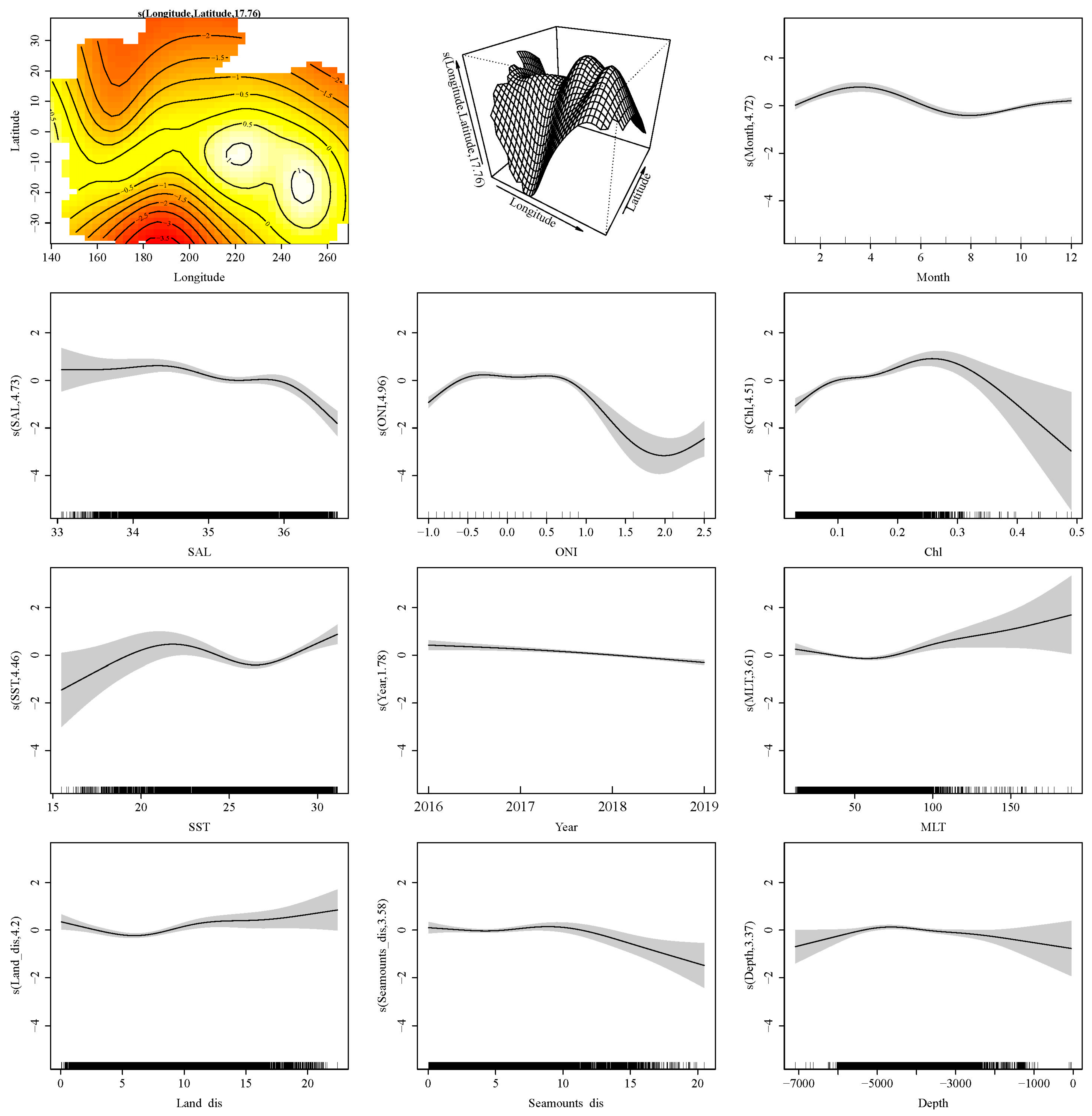
| Latitude * longitude | 17.762 | <0.001 | 10.84 |
| Month | 4.719 | <0.001 | 1.06 |
| SAL | 4.728 | <0.001 | 0.89 |
| ONI | 4.96 | <0.001 | 0.91 |
| Chl | 4.507 | <0.001 | 0.63 |
| SST | 4.457 | <0.001 | 0.36 |
| Year | 1.78 | <0.001 | 0.20 |
| MLT | 3.612 | <0.001 | 0.21 |
| Land_dis | 4.203 | <0.001 | 0.27 |
| Seamounts_dis | 3.578 | <0.001 | 0.18 |
| Depth | 3.369 | 0.023 | 0.10 |
Disclaimer/Publisher’s Note: The statements, opinions and data contained in all publications are solely those of the individual author(s) and contributor(s) and not of MDPI and/or the editor(s). MDPI and/or the editor(s) disclaim responsibility for any injury to people or property resulting from any ideas, methods, instructions or products referred to in the content. |
© 2023 by the authors. Licensee MDPI, Basel, Switzerland. This article is an open access article distributed under the terms and conditions of the Creative Commons Attribution (CC BY) license (https://creativecommons.org/licenses/by/4.0/).
Share and Cite
Wang, J.; Gao, C.; Wu, F.; Dai, L.; Ma, Q.; Tian, S. Environmental Characteristics Associated with the Presence of the Pelagic Stingray (Pteroplatytrygon violacea) in the Pacific High Sea. Fishes 2023, 8, 46. https://doi.org/10.3390/fishes8010046
Wang J, Gao C, Wu F, Dai L, Ma Q, Tian S. Environmental Characteristics Associated with the Presence of the Pelagic Stingray (Pteroplatytrygon violacea) in the Pacific High Sea. Fishes. 2023; 8(1):46. https://doi.org/10.3390/fishes8010046
Chicago/Turabian StyleWang, Jiaqi, Chunxia Gao, Feng Wu, Libin Dai, Qiuyun Ma, and Siquan Tian. 2023. "Environmental Characteristics Associated with the Presence of the Pelagic Stingray (Pteroplatytrygon violacea) in the Pacific High Sea" Fishes 8, no. 1: 46. https://doi.org/10.3390/fishes8010046
APA StyleWang, J., Gao, C., Wu, F., Dai, L., Ma, Q., & Tian, S. (2023). Environmental Characteristics Associated with the Presence of the Pelagic Stingray (Pteroplatytrygon violacea) in the Pacific High Sea. Fishes, 8(1), 46. https://doi.org/10.3390/fishes8010046