
Fishery Resource Evaluation in Shantou Seas Based on Remote Sensing and Hydroacoustics


Abstract
:
1. Introduction
2. Materials and Methods
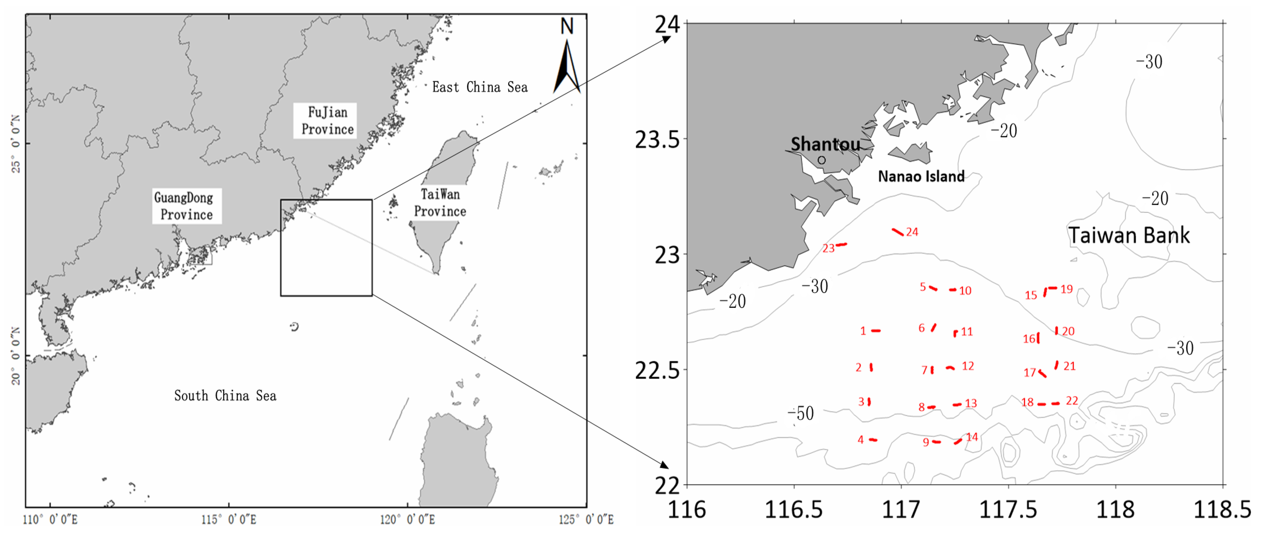
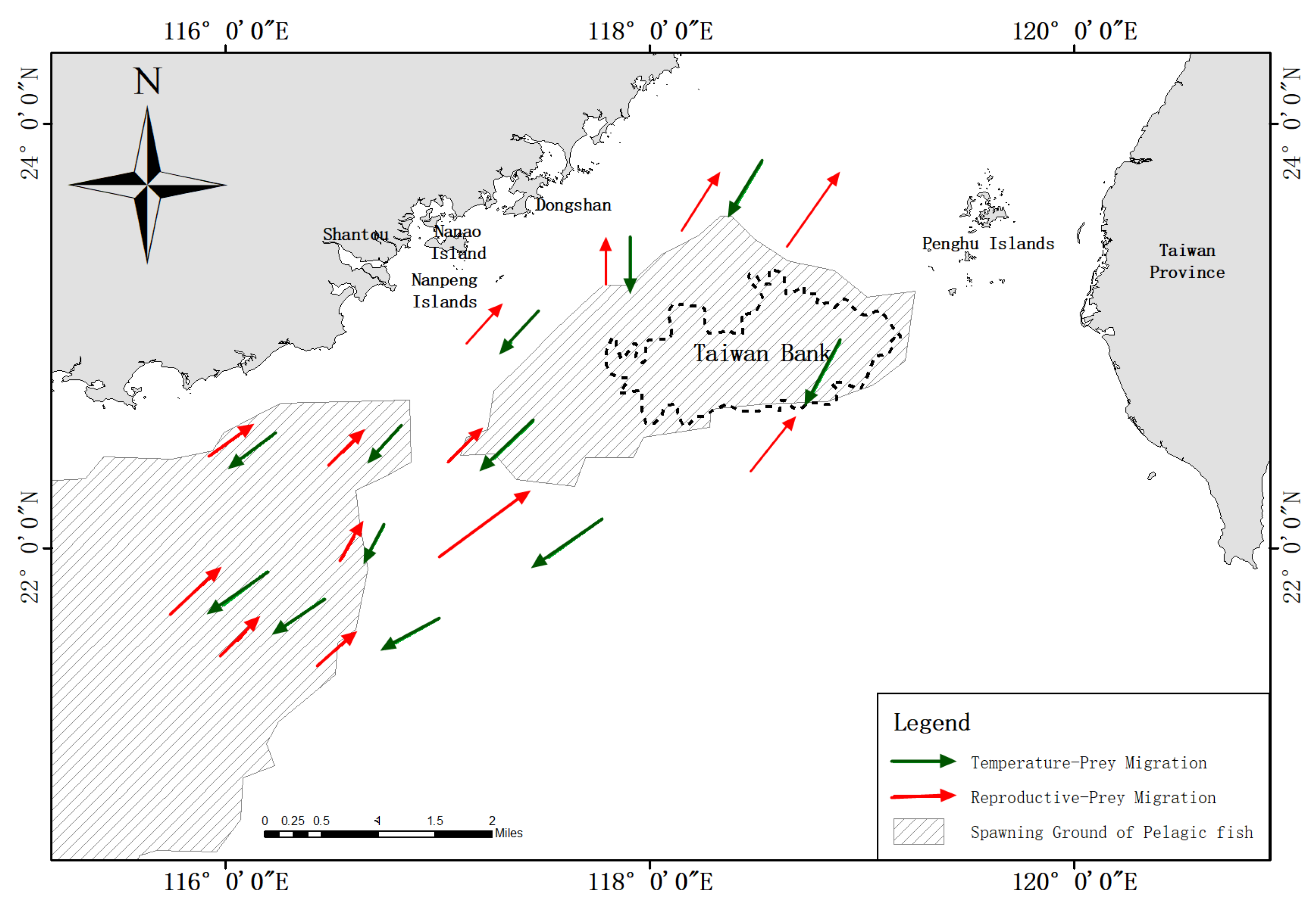
2.1. Study Area
2.2. Hydroacoustic Data
2.3. Remote Sensing Data
2.4. Variation Function and Kriging Interpolation
- (1)
- Verify the normality of fish density and acoustic biomass. If they do not meet, a log, square, or Box-Cox transformation was performed.
- (2)
- Onthe premise of isotropy, the semi-variogram function is modeled. These common models are spherical model, exponential model and Gaussian model. Each model can be described based on three parameters: (i) nugget variance, , the model Y-axis in-tercept; (ii) Sill, , the model asymptote; (iii) range, a, the distance over which spatial dependence is apparent. The regression coefficient ( and residual sums of squares (RSS) are indexs reflecting the precision of the fitting model.
- (3)
- After running all models, the model with the highest RSS values and smallest values was chosen to interpolate fish density and acoustic biomass. Kriging interpolation is performed based on the information provided by the variance function on the degree of spatial autocorrelation, so that optimal unbiased estimates can be obtained, while providing the error and accuracy of the estimates.
- (4)
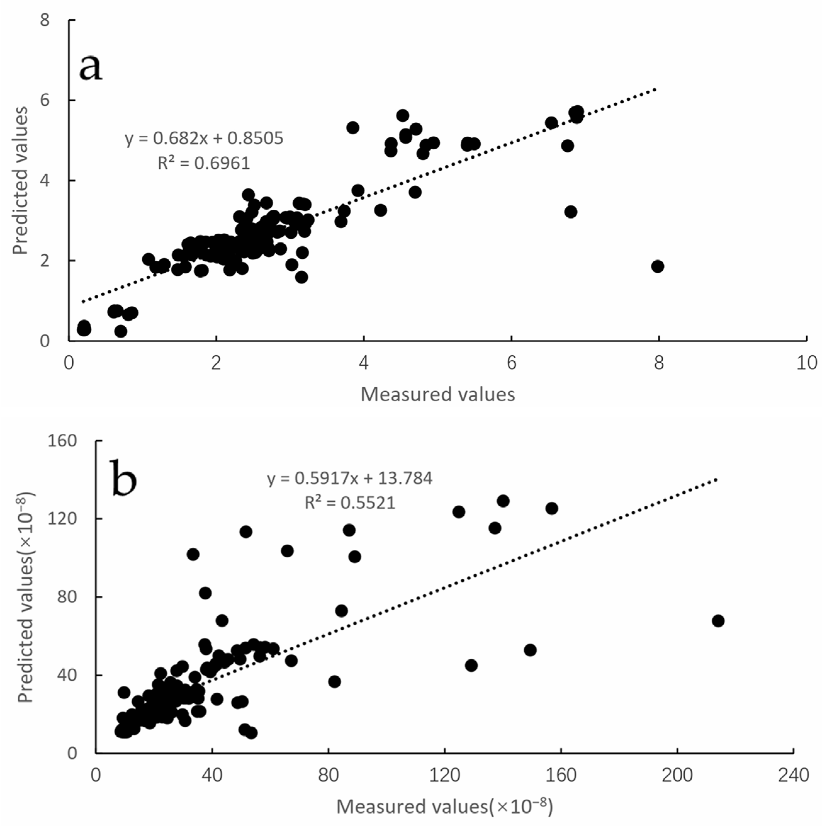
- Cross-validation was used to evaluate the result of kriging.
2.5. GAM Model
3. Results
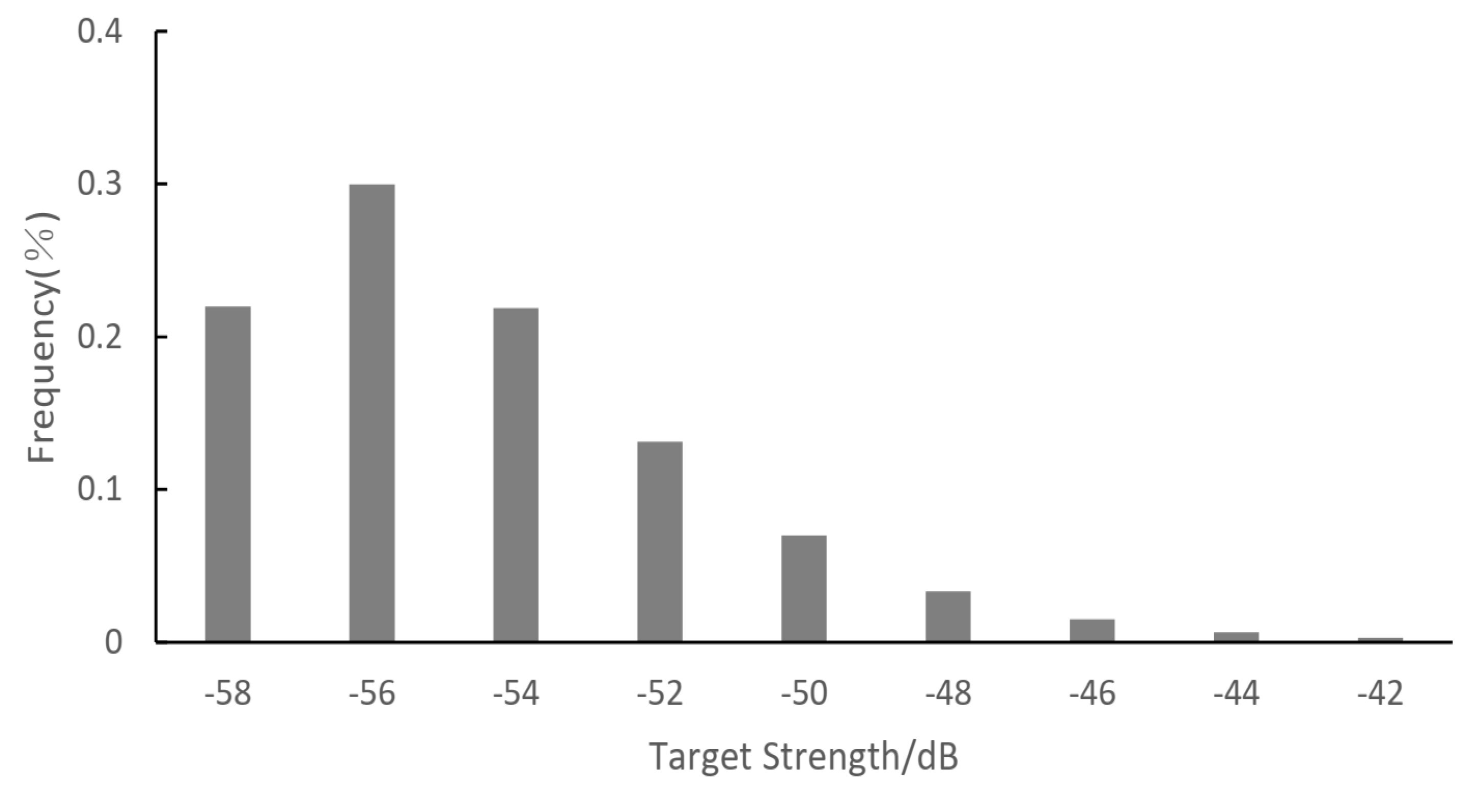
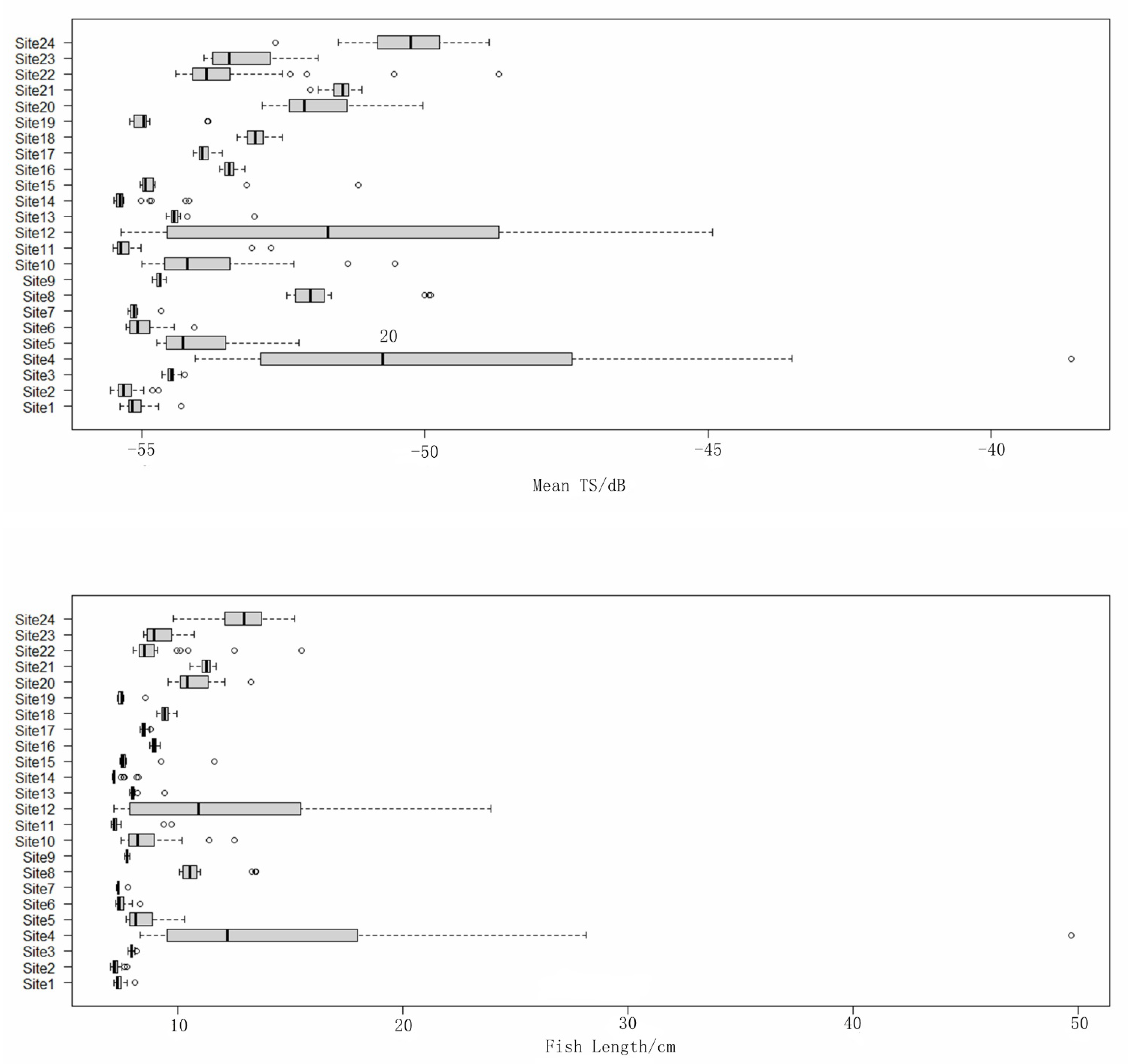
3.1. Fish Size Distribution
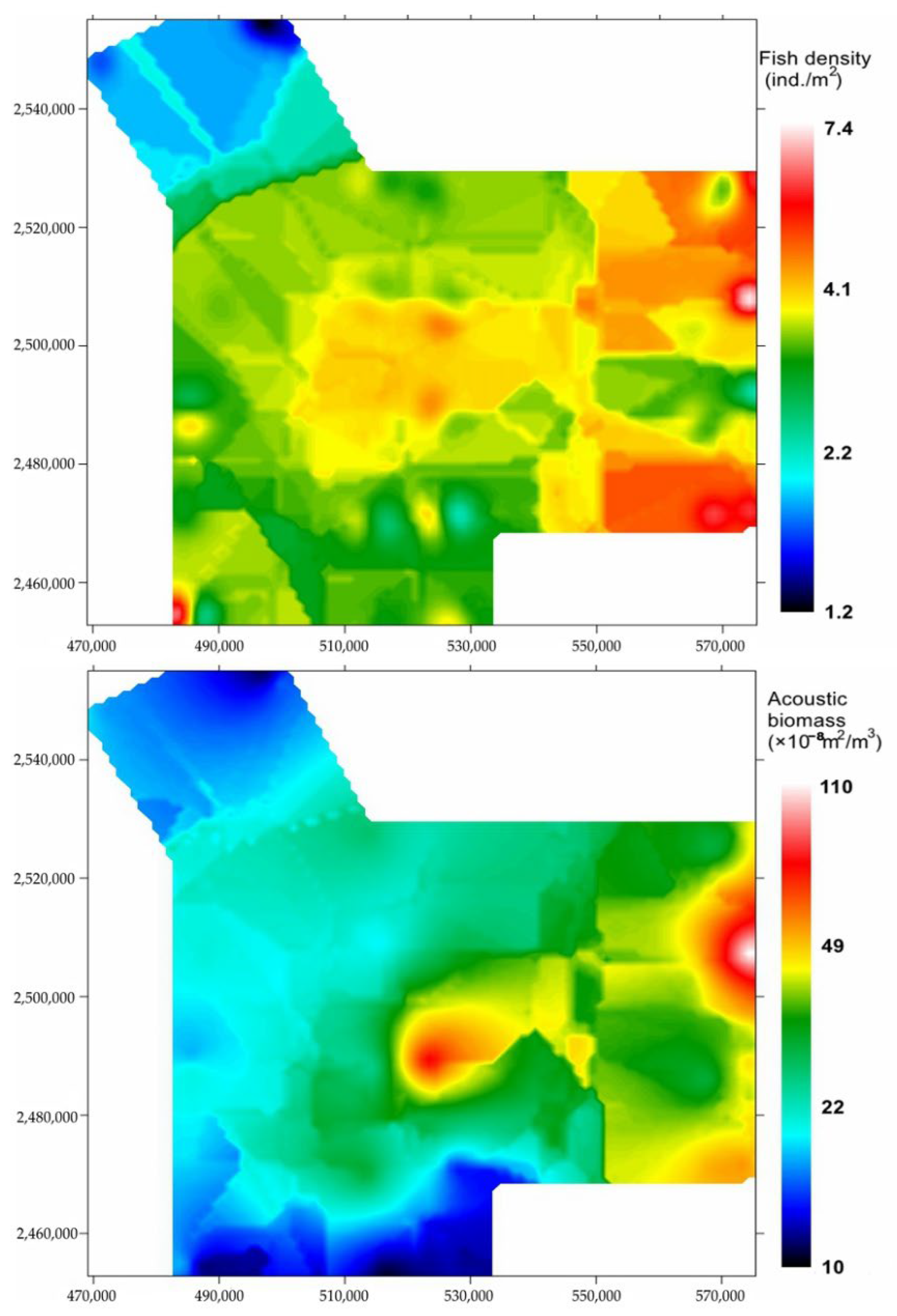
3.2. Spatial Distribution, Abundance and Biomass
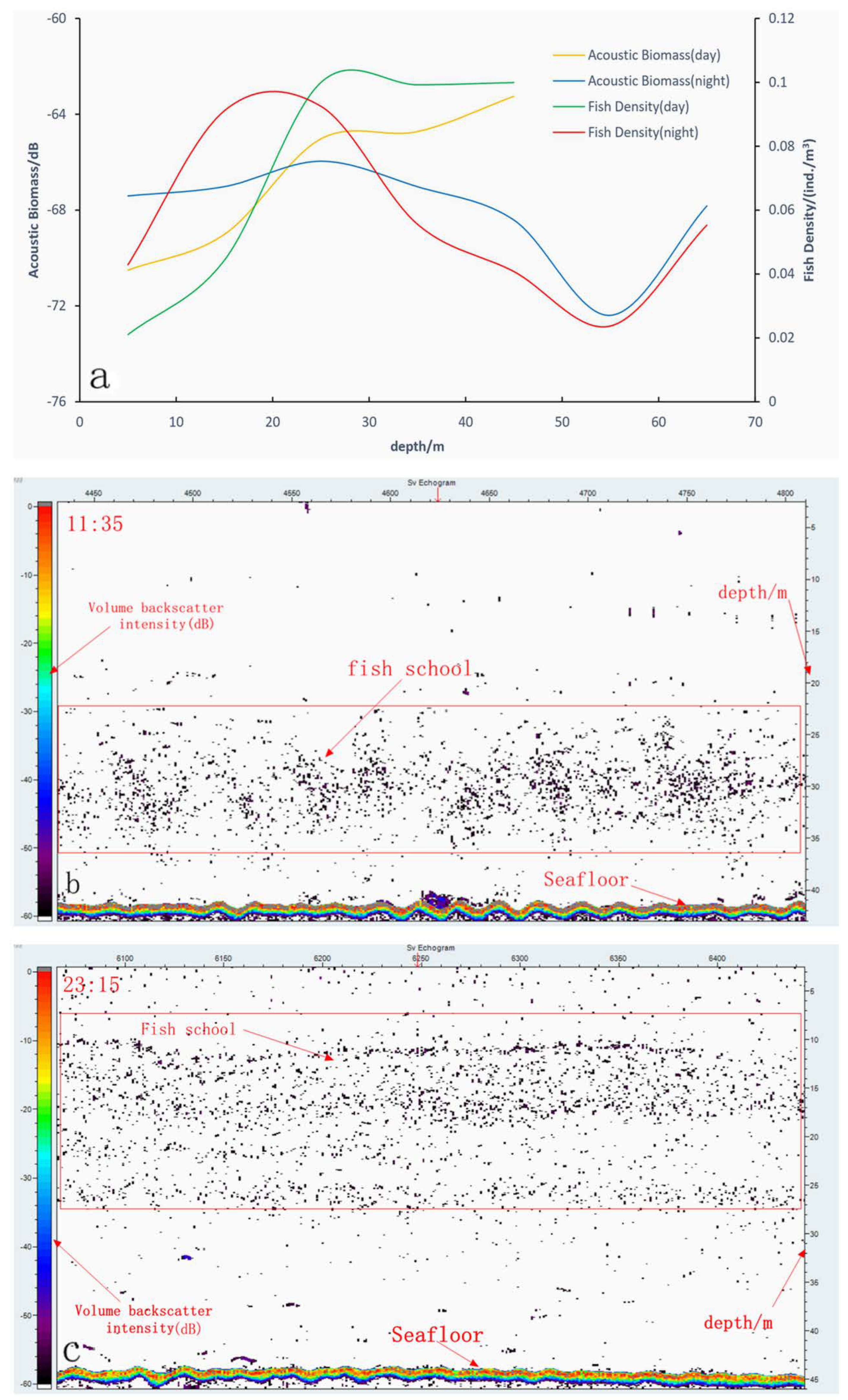
3.3. Vertical Distribution of Fish Density and Acoustic Biomass
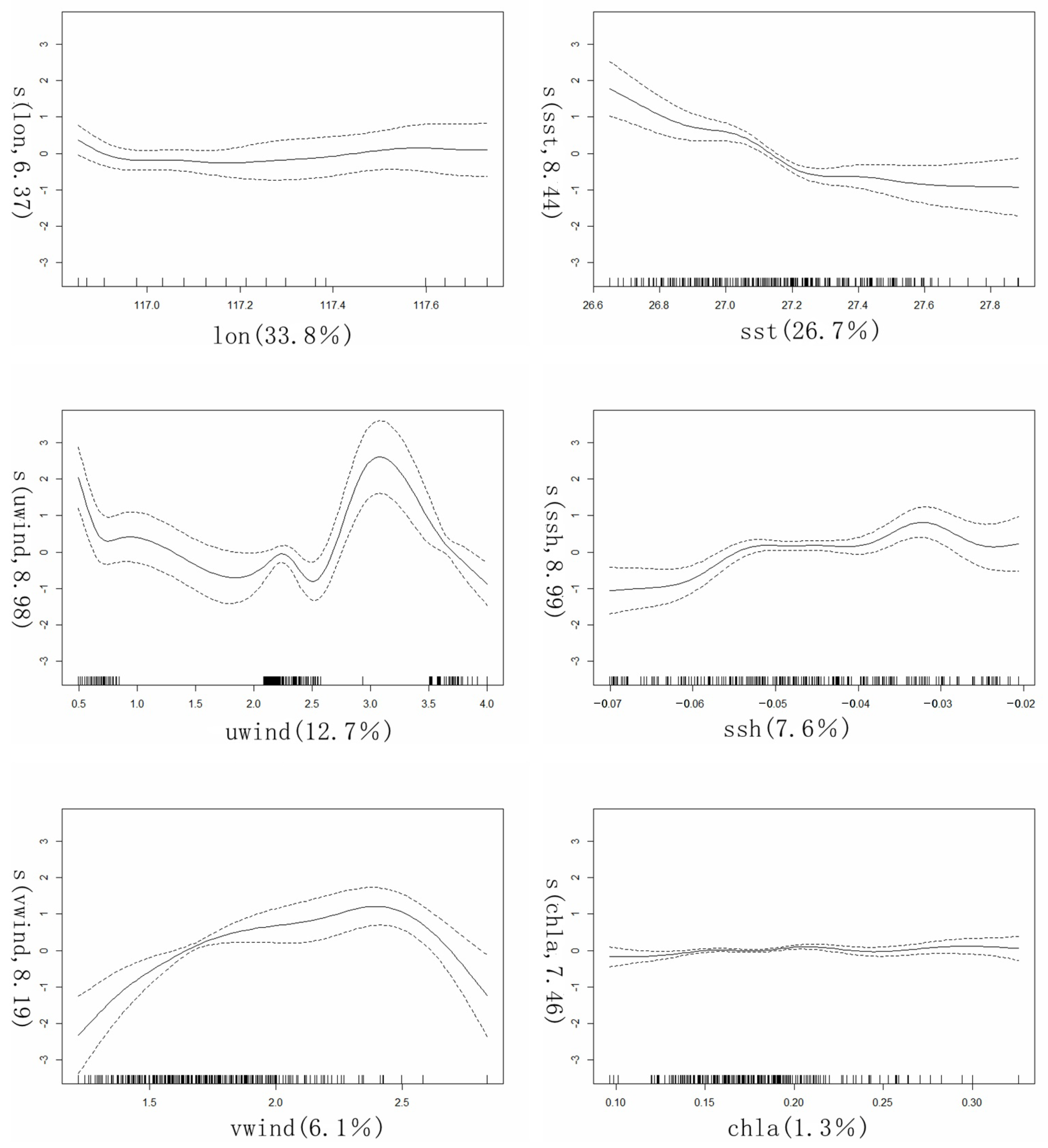
3.4. Fish Distribution Affected by Environmental Factors—GAM Model
4. Discussion
5. Conclusions
Author Contributions
Funding
Institutional Review Board Statement
Data Availability Statement
Conflicts of Interest
References
- Alheit, J.; Peck, M.A. Drivers of dynamics of small pelagic fish resources: Biology, management and human factor. Mar. Ecol. Prog. Ser. 2019, 617–618, 1–6. [Google Scholar] [CrossRef] [Green Version]
- Coll, M.; Palomera, I.; Tudela, S.; Dowd, M. Food-web dynamics in the South Catalan Sea ecosystem (NW Mediterranean) for 1978–2003. Ecol. Model. 2008, 217, 95–116. [Google Scholar] [CrossRef]
- Niu, M.; Li, X.; Zhao, G. Spatial distribution of wintering Engraulis japonicus and its relationship with the inter-annual variations of water temperature in central and southern Yellow Sea. China J. Appl. Ecol. 2011, 23, 552–558. [Google Scholar]
- Liu, S.; Liu, Y.; Alabia, I.D.; Tian, Y.; Ye, Z.; Yu, H.; Li, J.; Cheng, J. Impact of Climate Change on Wintering Ground of Japanese Anchovy (Engraulis japonicus) Using Marine Geospatial Statistics. Front. Mar. Sci. 2020, 7, 604. [Google Scholar] [CrossRef]
- Maria, P.G.; Marta, C.; Marta, A.-P.; Elena, F.-C.; Jeroen, S.; Ana, G.; María, G.; Antonio, E.; José, M.B. Current and Future Influence of Environmental Factors on Small Pelagic Fish Distributions in the Northwestern Mediterranean Sea. Front. Mar. Sci. 2020, 7, 622. [Google Scholar]
- Lu, Z.B.; Dai, Q.S.; Zhu, J.F.; Yan, Y.M. Changes in Structure of the Fisheries Resources and Ecology of the Major Population in Fujian Offshore Water. J. Fujian Fish 1999, 3, 1–7. [Google Scholar]
- Xiao, F.S. Fishery resources capacity in ecosystem of Minnan-Taiwan shoal Fishing Ground. J. Oceanogr. Taiwan Strait 2003, 22, 449–456. [Google Scholar]
- Hilborn, R.; Ovando, D. Reflections on the success of traditional fisheries management. ICES J. Mar. Sci. 2014, 71, 1040–1046. [Google Scholar] [CrossRef]
- Stockwell, J.D.; Yule, D.L.; Gorman, O.T.; Isaac, E.J.; Moore, S.A. Evaluation of Bottom Trawls as Compared to Acoustics to Assess Adult Lake Herring (Coregonus artedi) Abundance in Lake Superior. J. Great Lakes Res. 2006, 32, 280–292. [Google Scholar] [CrossRef]
- Liu, W.D.; Lin, Z.J.; Jiang, Y.E.; Huang, Z.R. Spatial distribution of demersal fishery resources in the continental shelf of the northern South China Sea. J. Trop. Oceanogr. 2011, 30, 95–103. [Google Scholar]
- Zhang, P.; Zeng, X.G.; Yang, S.; Tan, Y.G.; Yang, L.; Peng, C.H.; Yang, B.Z.; Zhang, X.F.; Yan, L. Analyses on fishing ground and catch composition of large-scale light falling-net fisheries in South China Sea. South China Fish. Sci. 2013, 9, 75–79. [Google Scholar]
- Shan, X.J.; Chen, Y.L.; Dai, F.Q.; Jin, X.S.; Yang, D.T. Variations in fish community structure and diversity in the sections of the central and southern Yellow Sea. Acta Ecol. Sin. 2014, 34, 377–389. [Google Scholar]
- Koslowa, J.A.; Davisonb, P.C. Productivity and Biomass of Fishes in the California Current Large Marine Ecosystem-Comparison of Fishery-Dependent and-Independent Time Series. Environ. Dev. 2016, 17 (Suppl. 1), 23–32. [Google Scholar] [CrossRef] [Green Version]
- Rustandi, Y.; Fahrudin, A.; Zairion; Arkham, M.N.; Zahid, A.; Hamdani, A.; Ramli, A.; Trihandoyo, A. Distribution fisheries resources of Small Island in Estuary Area: An assessment in Bunyu Island, North Kalimantan, Indonesia. IOP Conf. Ser. Earth Environ. Sci. 2019, 241, 012003. [Google Scholar] [CrossRef]
- Cai, Y.C.; Huang, Z.R.; Xu, Y.W.; Sun, M.S.; Xu, S.N.; Zhaang, K.; Chen, Z.Z. Probability distribution characteristics of stock density in offshore of northern South China Sea. China J. Appl. Ecol. 2019, 30, 2426–2436. [Google Scholar]
- Jens, O.; Eglė, J.; Olavi, K.; Niklas, L.; Ulf, B.; Michele, C.; Massimiliano, C.; Joakim, H.; Pär, B.; Emory, A. The first large-scale assessment of three-spined stickleback (Gasterosteus aculeatus) biomass and spatial distribution in the Baltic Sea. ICES J. Mar. Sci. 2019, 76, 1653–1665. [Google Scholar] [CrossRef]
- Lucca, B.M.; Warren, J.D. Fishery-independent observations of Atlantic menhaden abundance in the coastal waters south of New York. Fish Res. 2019, 218, 229–236. [Google Scholar] [CrossRef]
- Misund, O.A.; Aglen, A.; Frarnaes, E. Mapping the shape, size, and density of fish schools by echo integration and a high-resolution sonar. ICES J. Mar. Sci 1995, 52, 11–20. [Google Scholar] [CrossRef]
- Misund, O.A. Underwater acoustics in marine fisheries and fisheries research. Rev. Fish Biol. Fish. 1997, 7, 1–34. [Google Scholar] [CrossRef]
- Kubecka, J.; Duncan, A. Diurnal changes of fish behaviour in a lowland river monitored by a dual-beam echosounder. Fish Res. 1998, 35, 55–63. [Google Scholar] [CrossRef]
- Simard, Y.; Lavoie, D. The rich krill aggregation of the Saguenay-St. Lawrence Marine Park: Hydroacoustic and geostatistical biomass estimates, structure, variability, and significance for whales. J. Fish. Aquat. Sci. 1999, 56, 1182–1197. [Google Scholar] [CrossRef]
- Stanley, D.R.; Wilson, C.A. Variation in the density and species composition of fishes associated with three petroleum platforms using dual beam hydroacoustics. Fish Res. 2000, 47, 161–172. [Google Scholar] [CrossRef]
- Chen, G.; Chen, W.Z. The application of acoustic method in fishery resources survey. J. Shanghai Ocean Univ. 2003, 12, 40–44. [Google Scholar]
- Krumme, U.; Paul, U.S. Observations of fish migration in a macrotidal mangrove channel in Northern Brazil using a 200-kHz split-beam sonar. Aquat. Living Resour. 2003, 16, 175–184. [Google Scholar] [CrossRef]
- LI, Y.Z.; Chen, G.G.; Zhao, X.Y.; Chen, Y.Z.; Jin, X.S. Acoustic Assessment of Non-Commercial Small-Size Fish Resources in the Northern Waters of South China Sea. Period. Ocean. Univ. China 2005, 35, 206–212. [Google Scholar] [CrossRef]
- Chen, G.B.; Li, Y.Z.; Zhao, X.Y.; Chen, Y.Z.; Jin, X.S. Acoustic assessment of five groups commercial fish in South China Sea. Acta Oceanol. Sin. 2006, 28, 128–134. [Google Scholar]
- Godlewska, M.; Colon, M.; Doroszczyk, L.; Długoszewski, B.; Verges, C.; Guillard, J. Hydroacoustic measurements at two frequencies: 70 and 120 kHz–consequences for fish stock estimation. Fish Res. 2009, 96, 11–16. [Google Scholar] [CrossRef]
- Boswell, K.M.; Wilson, M.P.; MacRae, P.S.D.; Wilson, C.A.; Cowan, J.H. Seasonal Estimates of Fish Biomass and Length Distributions Using Acoustics and Traditional Nets to Identify Estuarine Habitat Preferences in Barataria Bay, Louisiana. Mar. Coast. Fish 2010, 2, 83–97. [Google Scholar] [CrossRef]
- Zhang, J.; Chen, P.M.; Fang, L.C.; Chen, G.B.; Li, X.G. Background acoustic estimation of fisheries resources in marine ranching area of Zhelin Bay-Nan’ao Island in the south China Sea. J. Fish. Sci. China 2015, 39, 1187–7798. [Google Scholar]
- Wang, D.X.; Chen, G.B.; Tang, Y.; Lin, B.; Wang, Z.C. Underwater Acoustics Assessment on Fishery Resources in the Southern Daya Bay. J. Anhui Agric. Sci. 2017, 45, 95–98. [Google Scholar] [CrossRef]
- Lian, Y.X.; Huang, G.; Godlewska, M.; Cai, X.W.; Li, C.; Ye, S.W.; Liu, J.S.; Li, Z.J. Hydroacoustic estimates of fish biomass and spatial distributions in shallow lakes. China J. Oceanol. Limnol. 2017, 36, 587–597. [Google Scholar] [CrossRef]
- Egerton, J.P.; Ansi, M.A.; Abdallah, M.; Walton, M.; Hayes, J.; Turner, J.; Erisman, B.; Al-Maslamani, I.; Mohammed, M.; Vay, L.L. Hydroacoustics to examine fish association with shallow offshore habitats in the Arabian Gulf. Fish. Res. 2018, 199, 127–136. [Google Scholar] [CrossRef] [Green Version]
- Perivolioti, T.M.; Frouzova, J.; Tušer, M.; Bobori, D. Assessing the Fish Stock Status in Lake Trichonis: A Hydroacoustic Approach. Water 2020, 12, 1823. [Google Scholar] [CrossRef]
- Wang, T.; Huang, H.H.; Zhang, P.; Zhang, S.F.; Wu, F.X.; Liu, Q.X.; Liao, X.L.; Xie, B. Coustic survey of fisheries resources and spatial distribution in Guishan wind farm area. J. Fish. China 2020, 27, 1496–1504. [Google Scholar] [CrossRef]
- Shi, Y.C.; Chen, X.J. A review of stock assessment methods on small pelagic fish. Mar. Fish. 2019, 41, 118–128. [Google Scholar]
- Chen, G.B.; Li, Y.Z. Distribution of the Carangidae fishes in the continental shelf waters of northern South China Sea. J. Shanghai Fish. Univ. 2003, 12, 146–151. [Google Scholar]
- Hixon, M.A.; Anderson, T.W.; Buch, K.L.; Johnson, D.W.; McLeod, J.B.; Stallings, C.D. Density dependence and population regulation in marine fish:a large-scale, long-term field manipulation. Ecol. Monogr. 2012, 82, 467–489. [Google Scholar] [CrossRef] [Green Version]
- Moron, G.; Galloso, P.; Gutierrez, D.; Torrejon-Magallanes, J. Temporal changes in mesoscale aggregations and spatial distribution scenarios of the Peruvian anchovy (Engraulis ringens). Deep Sea Res. Part II 2019, 159, 75–83. [Google Scholar] [CrossRef]
- Pierre, P.; Jürgen, A.; Peck, M.A.; Kristina, R.; Xabier, I.; Martin, H.; Jeroen, V.D.K.; Thomas, P.; Carola, W.; Iratxe, Z.; et al. Anchovy population expansion in the North Sea. Mar. Ecol. Prog. Ser. 2012, 444, 1–13. [Google Scholar]
- Ngando, N.E.; Song, L.; Cui, H.; Xu, S. Relationship Between the Spatiotemporal Distribution of Dominant Small Pelagic Fishes and Environmental Factors in Mauritanian Waters. J. Ocean Univ. China 2020, 19, 393–408. [Google Scholar] [CrossRef]
- Xu, Y.; Nietoa, K.; Teo, S.L.; McClatchie, S.; Holmesc, J. Influence of fronts on the spatial distribution of albacore tuna (Thunnus alalunga) in the Northeast Pacific over the past 30 years (1982–2011). Prog. Oceanogr. 2017, 150, 72–78. [Google Scholar] [CrossRef]
- Stenseth, N.C.; Mysterud, A.; Ottersen, G.; Hurrell, J.W.; Chan, K.-S.; Lima, M. Ecological Effects of Climate Fluctuations. Science 2002, 297, 1292–1296. [Google Scholar] [CrossRef] [PubMed] [Green Version]
- DingsØr, G.E.; Ciannelli, L.; Chan, K.-S.; Ottersen, G.; Stenseth, N.C. Density dependence and density independence during the early life stages of four marine fish stocks. Ecology 2007, 88, 625–634. [Google Scholar] [CrossRef] [PubMed]
- Ciannelli, L.; Chan, K.-S.; Bailey, K.M.; Stenseth, N.C. Nonadditive effects of the environment on the survival of a large marine fish population. Ecology 2004, 85, 3418–3427. [Google Scholar] [CrossRef] [Green Version]
- Wood, S.N. Generalized Additive Models: An Introduction with R. J. Stat. Softw 2006, 16, 135. [Google Scholar]
- Guan, W.J.; Chen, X.; Gao, F.; Li, G. Environmental effects on fishing efficiency of Scomber japonicus for Chinese large lighting purse seine fishery in the Yellow and East China Seas. J. Fish. Sci. China 2009, 16, 949–958. [Google Scholar]
- Li, G.; Chen, X.J. Relationship between mackerel yield and Marine environmental factors in East China Sea fishery in summer. J. Mar. Sci. 2009, 27, 1–8. [Google Scholar]
- Niu, M.x.; LI, X.S.; Xu, Y.C. Effects of spatiotemporal and environmental factors on the fishing ground of Trachurus murphyi in Southeast Pacific Ocean based on generalized additive model. Chin. J. Appl. Ecol. 2010, 21, 1049–1055. [Google Scholar] [CrossRef]
- Wang, S.Q.; Xu, L.X.; Zhu, G.P. Spatial-temporal profiles of CPUE andrelations to environmental factors for yellowfin tunaThunnus albacores from purse-seine fishery in Western and Central Pacific Ocean. J. Dalian Ocean Univ. 2014, 29, 303–308. [Google Scholar]
- Nieto, K.; Xu, Y.; Teo, S.L.H.; McClatchie, S.; Holmes, J. How important are coastal fronts to albacore tuna (Thunnus alalunga) habitat in the Northeast Pacific Ocean? Prog. Oceanogr. 2015, 150, 62–71. [Google Scholar] [CrossRef]
- Dai, S.W.; Tang, F.H.; Fan, W.; Zhang, H.; Cui, X.S.; Guo, G.G. Distribution of resource and environment characteristics of fishing ground of Scomber japonicas in the North Pacific high seas. Mar. Fish. 2017, 39, 372–382. [Google Scholar] [CrossRef]
- Fan, J.T.; Zhang, J.; Feng, X.; Chen, Z.Z. Relationship between Sthenoteuthis oualaniensis fishing ground and marine environmental factors in Nansha area. J. Shanghai Fish. Univ. 2019, 28, 419–426. [Google Scholar]
- Yang, S.L.; Fan, X.M.; Wu, Y.M.; Zhou, W.F.; Wang, F.; Wu, Z.L.; Zhang, B.B.; Fan, W. The relationship between the fishing ground of mackerel (Scomber australasicus) in Arabian Sea and the environment based on GAM model. Chin. J. Ecol. 2019, 38, 2466–2470. [Google Scholar]
- Zhou, G.F.; Xu, R.M. Biogeographic Statistics; Science Press: Beijing, China, 1997. [Google Scholar]
- Rossi, R.E.; Mulla, D.J.; Journel, A.G.; Franz, E.H. Geostatistical Tools for Modeling and Interpreting Ecological Spatial Dependence. Ecol. Monogr. 1992, 62, 277–314. [Google Scholar] [CrossRef]
- Matheron, G. Principles of Geostatistics. Econ. Geol. 1963, 58, 1246–1266. [Google Scholar] [CrossRef]
- Chen, X.J.; Fang, X.Y.; Yang, M.X.; Feng, Y.J.; Jia, T. Application of Geostatistics in Marine Fisheries; Science Press: Beijing, China, 2019. [Google Scholar]
- Li, L.; Wang, L.; Liu, Q.; Huang, H. Geostatistical analysis of tuna (Thunnus obesus) longline fishing grounds in the Atlantic Ocean. J. Fish. Sci. China 2013, 20, 198–204. [Google Scholar] [CrossRef]
- Otilio, A.; Iván, V.A.; Carlos, F.J.; Enrique, Á.G.L.; Alvaro, H.-F.; Ángel, G. Biomass and distribution of the red octopus (Octopus maya) in the north-east of the Campeche Bank. J. Mar. Biol. Assoc. U. K. 2019, 99, 1317–1323. [Google Scholar] [CrossRef] [Green Version]
- Castillo, R.; Aparco, L.L.C.; Grados, D.; Cornejo, R.; Guevara, R.; Csirke, A.J. Anchoveta (Engraulis ringens) Biomass in the Peruvian Marine Ecosystem Estimated by Various Hydroacoustic Methodologies during spring of 2019. J. Mar. Biol. Oceanogr. 2020, 9, 35–55. [Google Scholar]
- Roa-Ureta, R.N.; Niklitschek, E. Biomass estimation from surveys with likelihood-based geostatistics. ICES J. Mar. Sci. 2007, 64, 1723–1734. [Google Scholar] [CrossRef] [Green Version]
- Stratis, G.; Dimitra, K. Mapping abundance distribution of small pelagic species applying hydroacoustics and Co-Kriging techniques. Hydrobiologia 2008, 612, 155–169. [Google Scholar] [CrossRef]
- Sullivan, P.J. Stock Abundance Estimation Using Depth- Dependent Trends and Spatially Correlated Variation. Can. J. Fish. Aquat. Sci. 1991, 48, 1691–1703. [Google Scholar] [CrossRef]
- Simard, Y.; Legendre, P.; Lavoie, G.; Marcotte, D. Mapping, estimating biomass, and optirnizing sampling programs for spatially autocorrelated data: Case study ofthe northern shrimp (Pandalus borealis). Can. J. Fish. Aquat. Sci. 1992, 49, 32–45. [Google Scholar] [CrossRef]
- Simard, Y.; Marcotte, D.; Bourgault, G. Exploration of geostatistical methods for mapping and estirnating acoustic biomass of pelagic fish in the Gulf of St. Lawrence: Size of echo-integration unit and auxiliary environmental variables. Aquat. Living Res. 1993, 6, 185–199. [Google Scholar] [CrossRef]
- Páramo, J.; Roa, R. Acoustic-geostatistical assessment and habitat–abundance relations of small pelagic fish from the Colombian Caribbean. Fish. Res. 2003, 60, 309–319. [Google Scholar] [CrossRef]
- Petitgas, P. Geostatistics in fisheries survey design and stock assessment: Models, variances and applications. Fish Fish. 2001, 2, 231–249. [Google Scholar] [CrossRef]
- Su, F.Z.; Zhou, C.; Zhang, T.Y.; Du, Y.Y.; Yao, C.Q. Spatial heterogeneity of pelagic fishery resources in the East China Sea. Chin. J. Appl. Ecol. 2003, 14, 1971–1975. [Google Scholar]
- Wu, Z.; Zhang, C.L.; Xue, Y.; Ji, Y.P.; Ren, Y.P.; Xu, B.D. Spatial heterogeneity of demersal fish in the offshore waters of Shandong. Haiyang Xuebao 2022, 44, 21–28. [Google Scholar]
- Addis, P.; Secci, M.; Angioni, A.; Cau, A. Spatial distribution patterns and population structure of the sea urchin Paracentrotus lividus (Echinodermata: Echinoidea), in the coastal fishery of western Sardinia: A geostatistical analysis. Sci. Mar. 2011, 76, 733–740. [Google Scholar] [CrossRef] [Green Version]
- Saraux, C.; Fromentin, J.-M.; Bigot, J.-L.; Bourdeix, J.-H.; Morfin, M.; Roos, D.; Beveren, E.V.; Bez, N. Spatial Structure and Distribution of Small Pelagic Fish in the Northwestern Mediterranean Sea. PLoS ONE 2014, 9, e111211. [Google Scholar] [CrossRef]
- Zhu, W.; Lu, K.; Lu, Z.; Dai, Q.; Li, Z.; Zhou, Y.; Huang, S.; Zhu, H.; Cui., G. Implementing geostatistical analysis to study spatio-temporal distribution patterns of swimming crabs (Portunus trituberculatus). Acta Oceanol. Sin. 2021, 40, 67–74. [Google Scholar] [CrossRef]
- Rueda, M. Spatial distribution of fish species in a tropical estuarine lagoon: A geostatistical appraisal. Mar. Ecol. Prog. Ser. 2001, 222, 217–226. [Google Scholar] [CrossRef]
- Maynou, F.X.; Sarda, F.; Conan, G.R.Y. Assessment of the spatial structure and biomass evaluation of Nephrops norvegicus (L.) populations in the northwestern Mediterranean by geostatistics. ICES J. Mar. Sci. 1998, 55, 102–120. [Google Scholar] [CrossRef] [Green Version]
- Pierre, P. Geostatistics for fish stock assessments: A review and an acoustic application. ICES J. Mar. Sci. 1993, 93, 285–298. [Google Scholar]
- Simard, Y.; Lavoie, D.; Saucier, F.J. Channel head dynamics: Capelin (Mallotus villosus) aggregation in the tidally driven upwelling system of the Saguenay-St. Lawrence Marine Park′s whale feeding ground. Can. J. Fish. Aquat. Sci. 2002, 59, 197–210. [Google Scholar] [CrossRef]
- Lin, X.Y. Present situation of fishery ecological environment and fishery resources in shantou Taiwan shoal fishery ground. Shantou Sci. Technol. 2007, 2, 29–32. [Google Scholar]
- Shang, S.P.; Hong, H.S.; Zhang, X.M.; Zhang, C.Y. On the potential relationship of fishing ground position shift with the variability of sea surface temperature in Taiwan strait in summers of 1997 and 1998. Mar. Sci. 2002, 26, 27–30. [Google Scholar]
- Fang, S.M.; Yang, S.Y.; Zhang, C.M.; Zhu, J.F. Effects of submarine topography and water depth on distribution of pelagic fish community in Minnan-Taiwan bank fishing ground. China J. Appl. Ecol. 2002, 13, 1463–1467. [Google Scholar]
- Li, X.D. Monthly Variability in the Catchability of Chub Macherel and Round Scad and Its Relationship with Environmental Seasonality in Southern Taiwan Strait; Xiamen University: Xiamen, China, 2006. [Google Scholar]
- Lin, X.Y. Assessment of pelagic fish resources, Carangidae fish resources and its maximum sustainable yield in the Shantou-Taiwan shoal fishing grounds. Fish. Sci. Technol. 2008, 2008, 28–30. [Google Scholar]
- Sun, M.B.; Gu, X.H.; Zeng, Q.F.; Mao, Z.G.; Gu, X.K. Assessment of fish spatial distribution and biomass in Lake Taihu using hydroacoustic method. J. Lake Sci. 2013, 25, 99–107. [Google Scholar]
- Simmonds, J.E.; Maclennan, D.N. Fisheries Acoustics: Theory and Practice, 2nd ed.; John Wiley & Sons: Hoboken, NJ, USA, 2007. [Google Scholar]
- Johnson, J.B.; Omland, K.S. Model selection in ecology and evolution. Trends Ecol. Evol. 2004, 19, 101–108. [Google Scholar] [CrossRef]
- Sakamoto, Y.; Ishiguro, M.; Kitagawa, G. Akaike Information Criterion Statistics; Kluwer Academic Publishers Group: Dordrecht, The Netherlands, 1986. [Google Scholar]
- Dai, T.; Su, Y.; Ruan, W.; Liao, Z. Conservation and Management of Fishery Resources in Taiwan Strait and Its Adjacent Sea Area; Xiamen University press: Xiamen, China, 2011. [Google Scholar]
- Li, B.; Chen, G.B.; Yu, J.; Wang, D.; Guo, Y.; Wang, Z.C. The acoustic survey of fisheries resources for various seasons in the mouth of Lingshui Bay of Hainan Island. J. Fish. China 2018, 42, 544–566. [Google Scholar] [CrossRef]
- Zeng, L.; Chen, G.B.; Jie, Y. Acoustic assessment of fishery resources and spatial distribution in Nan’ao Island area. South China Fish. Sci. 2018, 14, 26–35. [Google Scholar]
- Chen, G.B.; Li, Y.Z.; Chen, P.M. A study on spawning ground of blue mackerel scad (Decapterus maruadsi) in continental shelf waters of northern South China Sea. J. Trop. Oceanogr. 2003, 22, 22–28. [Google Scholar]
- Zhang, J.S. Mackerel in the northern South China Sea. Mar. Fish. 1980, 1, 1–4. [Google Scholar]
- Zhang, R.Z. Spawning grounds and spawning period of mackerel in the northern South China Sea. Fish. Sci. Technol. Inf. 1981, 6–9. [Google Scholar]
- Marine Fishery Waters Map of China: Fishery Waters Map of South Sea Region. China Fish. 2002, 6, 22–24.
- Gong, J.K. Migration, distribution and biological characteristics of squid in Minnan-Taiwan Shoal fishery. J. Fujian Fish 1981, 2, 17–28. [Google Scholar]
- Zhu, Y. Study on the characteristics of pelagic fish resources in Minnan-Taiwan Shoal fishing ground. J Fujian Fish 1981, 2, 5–14. [Google Scholar]
- Xiao, L. Study on the Changes of Fishery Resources and Ecological Characteristics of Pelagic Fishes in the Minnan-Taiwan Bank Fishing Ground; Xiamen University: Xiamen, China, 2013. [Google Scholar]
- Gu, D.X.; Liu, G.S.; Wang, X.Y.; Wang, T.; You, H.Z.; Qian, H.; Xu, H.L. Preliminary Study on Fish Resources and Its Relationship with Environmental Factors in Tianjin Sea Area Based on Generalized Additive Mode (GAM). J. Tianjin Agric. Univ. 2017, 24, 38–45. [Google Scholar]
- Ma, J.; Huang, J.L.; Chen, J.H.; Gao, C.X.; Wang, X.F.; Li, B.; Zhao, J.; Tian, S.Q. Analysis of spatiotemporal fish density distribution and its influential factors based on generalized additive model (GAM) in the Yangtze River estuary. J. Fish. China 2020, 44, 936–946. [Google Scholar] [CrossRef]
- Lu, W.Q.; Yuan, M.Z. The literature review of temperature change effect on fish behavior. J. Shanghai Fish. Univ. 2017, 26, 828–835. [Google Scholar]
- Fisheries Resources Survey Team. A review of Minnan-Taiwan Shoal fishing ground. J. Fujian Fish 1980, 1, 7–16.
- Wang, C.J.; Zhou, L.J.; Li, G. Analysis of the inter-annual variation of chub mackerel abundance in the East China Sea and Yellow Sea during 1999–2011. J. Fish. Sci. China 2014, 38, 56–64. [Google Scholar]
- Yi, W.; Guo, A.; Chen, X.J. A study on influence of different environmental factors weights on the habitat model for Scomber japonicus. Acta Oceanol. Sin. 2017, 38, 90–97. [Google Scholar]
- Chen, X.; Fan, W. Applied Theory and Technology of Fishery Remote Sensing; Science Press: Beijing, China, 2015. [Google Scholar]
- Zhuang, W.; Wang, D.X.; Wu, R.S.; Hu, J.Y. Coastal Upwelling off Eastern Fujian-Guangdong Detected by Remote Sensing. Chin. J. Atmos. Sci. 2005, 29, 438–444. [Google Scholar]
- Miranda, E.H.; Palma, A.T.; Ojeda, F.P. Larval fish assemblages in nearshore coastal waters off central Chile: Temporal and spatial patterns. Estuar. Coast. Shelf Sci. 2003, 56, 1075–1092. [Google Scholar] [CrossRef]
- Voss, R.; Hinrichsen, H.H. Sources of uncertainty in ichthyoplankton surveys: Modeling the influence of wind forcing and survey strategy on abundance estimates. J. Mar. Syst. 2003, 43, 87–103. [Google Scholar] [CrossRef]
- Comerford, S.; Brophy, D. The role of wind-forcing in the distribution of larval fish in Galway Bay, Ireland. J. Mar. Biol. Assoc. U. K. 2013, 93, 471–478. [Google Scholar] [CrossRef]
- Chen, J.Q.; Fu, Z.; LI, F.X. Study on upwelling in Minnan-Taiwan shoal fishery. J. Oceangr. Taiwan Strait 1982, 1, 5–13. [Google Scholar]
- Fu, Z.L. Upwelling in the Taiwan Strait. Mar. Sci. 1984, 2, 54–56. [Google Scholar]
- Wu, Y.C.; Wong, X.Z.; Yang, Y.L. Analysis on causes of generation, evolution and decay process of upwelling off the western coast of Taiwan strait. Stud. Mar. Sin. 1997, 38, 53–59. [Google Scholar]
- Chen, G.H. Influence of wind on hydrological structure and upwelling in spring and summer along the central coast of Fujian. Mar. Sci. 1991, 4, 50–55. [Google Scholar]
- Song, T. Relationship beween Fishing Ground of Ommastrephes Bartrami and Satellite Altimeter Data in Northwestern Pacific; Shanghai Ocean University: Shanghai, China, 2014. [Google Scholar]
- Koschinski, S.; Culik, B.M.; Henriksen, O.D.; Tregenza, N.; Ellis, G.; Jansen, C.; Kathe, G. Behavioural reactions of free-ranging porpoises and seals to the noise of a simulated 2 MW windpower generator. Mar. Ecol. Prog. Ser. 2003, 265, 263–273. [Google Scholar] [CrossRef] [Green Version]
- Gill, A.B. Offshore renewable energy: Ecological implications of generating electricity in the coastal zone. J. Appl. Ecol. 2005, 42, 605–615. [Google Scholar] [CrossRef] [Green Version]
- Wahlberg, M.; Westerberg, H. Hearing in fish and their reactions to sounds from offshore wind farms. Mar. Ecol. Prog. Ser. 2005, 288, 295–309. [Google Scholar] [CrossRef]
- Thomsen, F.; Lüdemann, K.; Kafemann, R.; Piper, W. Effects of Offshore Wind Farm Noise on Marine Mammals and Fish; COWRIE Ltd.: Hanbury, Germany, 2006. [Google Scholar]
- Zettler, M.L.; Pollehne, F. The impact of wind engine constructions on benthic growth patterns in the western Baltic. In Offshore Wind Energy; Springer: Berlin/Heidelberg, Germany, 2006; pp. 201–222. [Google Scholar]
- Bergström, L.; Kautsky, L.; Malm, T.; Rosenberg, R.; Wahlberg, M.; Capetillo, N.Å.; Wilhelmsson, D. Effects of offshore wind farms on marine wildlife-a generalized impact assessment. Environ. Res. Lett. 2014, 9, 2033–2053. [Google Scholar] [CrossRef]
- Halouani, G.; Villanueva, C.M.; Raoux, A.; Dauvin, J.C.; Lasram, F.B.R.; Foucher, E.; Loc’h, F.L.; Safi, G.; Araignous, E.; Robin, J.P.; et al. A spatial food web model to investigate potential spillover effects of a fishery closure in an offshore wind farm. J. Mar. Syst. 2020, 212, 103434. [Google Scholar] [CrossRef]
- Wilhelmsson, D.; Malm, T.; Ohman, M.C. The influence of offshore windpower on demersal fish. ICES J. Mar. Sci 2006, 63, 775–784. [Google Scholar] [CrossRef] [Green Version]
- Fayram, A.H.; Risi, A.D. The potential compatibility of offshore wind powerand fisheries: An example using bluefin tunain the Adriatic Sea. Ocean. Coast Manag. 2007, 50, 597–605. [Google Scholar] [CrossRef]
- Punt, M.J.; Groeneveld, R.A.; Ierland, E.C.V.; Stel, J.H. Spatial planning of offshore wind farms: A windfall to marine environmental protection? Ecol. Econ. 2009, 69, 93–103. [Google Scholar] [CrossRef]
- Berkel, J.V.; Burchard, H.; Christensen, A.; Mortensen, L.O.; Thomsen, F. The Effects of Offshore Wind Farms on Hydrodynamics and Implications for Fishes. Oceanography 2020, 33, 108–117. [Google Scholar] [CrossRef]
- Tian, S.Q.; Chen, X.J.; Feng, B.; Qian, W.G. Spatio-temporal distribution of abundance index for Ommastrephes bartramii and its relationship with habitat environmental in the Northwest Pacific Ocean. J. Shanghai Fish. Univ. 2009, 18, 586–592. [Google Scholar]

| Station | Length (nm) | Station | Length (nm) | Station | Length (nm) |
|---|---|---|---|---|---|
| 1 | 2.39 | 9 | 2.59 | 17 | 2.67 |
| 2 | 2.12 | 10 | 1.80 | 18 | 2.18 |
| 3 | 2.46 | 11 | 2.42 | 19 | 2.71 |
| 4 | 2.18 | 12 | 2.54 | 20 | 2.45 |
| 5 | 2.54 | 13 | 2.20 | 21 | 2.52 |
| 6 | 2.44 | 14 | 2.34 | 22 | 2.37 |
| 7 | 2.27 | 15 | 2.56 | 23 | 2.93 |
| 8 | 2.17 | 16 | 3.04 | 24 | 3.59 |
| Variables | Units | Mean | Range | Description |
|---|---|---|---|---|
| SST | °C | 27.51 | 26.65–27.9 | Sea surface temperature |
| Chlorophyll-a | mg/m3 | 0.229 | 0.1093–1.123 | Chlorophyll concentration |
| uwind | m/s | 2.23 | 0.59–3.82 | Zonal sea surface wind |
| vwind | m/s | 1.6 | 0.52–2.18 | Meridional sea surface wind |
| SSTA | °C | 0.99 | 0.44–1.66 | Sea surface temperature anomaly |
| SSH | m | −0.0456 | −0.087–0.02 | Sea surface high |
| Model | R2 | AIC |
|---|---|---|
| Log(FPUA)~s(lon) | 0.314 | 33.081 |
| Log(FPUA)~s(lon)+s(sst) | 0.576 | −72.554 |
| Log(FPUA)~s(lon)+s(sst)+s(uwind) | 0.701 | −147.451 |
| Log(FPUA)~s(lon)+s(sst)+s(uwind)+s(ssh) | 0.775 | −204.835 |
| Log(FPUA)~s(lon)+s(sst)+s(uwind)+s(ssh)+s(vwind) | 0.84 | −279.005 |
| Log(FPUA)~s(lon)+s(sst)+s(uwind)+s(ssh)+s(vwind)+s(chla) | 0.851 | −291.111 |
| Variances | Max | Min | Mean | Kurtosis | Skewness | Standard Deviation | Coefficient of Variation |
|---|---|---|---|---|---|---|---|
| Acoustic biomass | 2.14 × 10⁻⁶ m2/m3 | 8.6 × 10⁻⁸ m2/m3 | 3.43 × 10⁻⁷ m2/m3 | 10.49 | 2.95 | 3.17 | 0.92 |
| Fish density | 7.98 ind./m2 | 0.20 ind./m2 | 2.70 ind./m2 | 2.344 | 1.281 | 1.43 | 0.53 |
| Model | Fish Density | Acoustic Biomass | ||||
|---|---|---|---|---|---|---|
| Exponential | Spherical | Gaussian | Exponential | Spherical | Gaussian | |
| Nugget (C0) | 0.0133 | 0.0074 | 0.0172 | 0.171 | 0.0802 | 0.0968 |
| Sill (C0 + C) | 0.0996 | 0.0928 | 0.0934 | 0.579 | 0.3704 | 0.3686 |
| Range (A)/m | 37,200 | 19,500 | 17,493.71 | 168,900 | 19,600 | 14,849.23 |
| RSS | 0.008991 | 0.008727 | 0.008635 | 0.158 | 0.186 | 0.185 |
| R2 | 0.413 | 0.430 | 0.436 | 0.385 | 0.279 | 0.280 |
| Proportion (C/(C0 + C) | 0.866 | 0.816 | 0.816 | 0.705 | 0.783 | 0.737 |
| Vaiables | Edf | F | p-Value | R2 | Deviance Explained/% | Cumulation of Deviance Explained/% | AIC |
|---|---|---|---|---|---|---|---|
| Lon | 6.366 | 6.663 | 4.08 × 10⁻⁶ | 0.314 | 33.8 | 33.8 | 33.081 |
| sst | 8.438 | 7.516 | 1.96 × 10⁻⁹ | 0.576 | 26.7 | 60.5 | −72.554 |
| uwind | 8.980 | 19.016 | 2 × 10⁻¹⁶ | 0.701 | 12.7 | 73.2 | −147.451 |
| ssh | 8.986 | 11.729 | 1.91 × 10⁻¹⁰ | 0.775 | 7.6 | 80.8 | −204.835 |
| vwind | 8.194 | 8.03 | 5.58 × 10⁻¹⁰ | 0.84 | 6.1 | 86.9 | −279.005 |
| chla | 7.460 | 1.992 | 0.0411 | 0.851 | 1.3 | 88.2 | −291.111 |
Publisher’s Note: MDPI stays neutral with regard to jurisdictional claims in published maps and institutional affiliations. |
© 2022 by the authors. Licensee MDPI, Basel, Switzerland. This article is an open access article distributed under the terms and conditions of the Creative Commons Attribution (CC BY) license (https://creativecommons.org/licenses/by/4.0/).
Share and Cite
Yin, X.; Yang, D.; Du, R. Fishery Resource Evaluation in Shantou Seas Based on Remote Sensing and Hydroacoustics. Fishes 2022, 7, 163. https://doi.org/10.3390/fishes7040163
Yin X, Yang D, Du R. Fishery Resource Evaluation in Shantou Seas Based on Remote Sensing and Hydroacoustics. Fishes. 2022; 7(4):163. https://doi.org/10.3390/fishes7040163
Chicago/Turabian StyleYin, Xiaoqing, Dingtian Yang, and Ranran Du. 2022. "Fishery Resource Evaluation in Shantou Seas Based on Remote Sensing and Hydroacoustics" Fishes 7, no. 4: 163. https://doi.org/10.3390/fishes7040163
APA StyleYin, X., Yang, D., & Du, R. (2022). Fishery Resource Evaluation in Shantou Seas Based on Remote Sensing and Hydroacoustics. Fishes, 7(4), 163. https://doi.org/10.3390/fishes7040163