Assessing the Effects of Species, Origin, and Processing on Frog Leg Meat Composition with Predictive Modeling Tools

Abstract

This study investigates the effects of species, geographical origin, and processing on the proximate composition of frog leg meat, with a focus on developing predictive models for processing status. Data were systematically compiled from 18 published studies, yielding 32 entries across 10 edible frog species and multiple processing methods. Proximate composition parameters (moisture, protein, fat, ash) were compared between processed and unprocessed samples, and classification models were trained using moisture content as the primary predictor. Logistic regression and several machine learning algorithms, including Stochastic Gradient Descent, Support Vector Machine, Random Forest, and Decision Tree, were benchmarked under a Leave-One-Study-Out (LOSO) cross-validation framework. Results demonstrated that moisture content alone was sufficient to accurately distinguish processing status, with a critical threshold of ~73% separating processed from unprocessed frog legs. Logistic regression achieved perfect specificity and precision (100%) with an overall accuracy of 96.8%, while other classifiers also performed strongly (>90% accuracy). These findings confirm moisture as a species- and origin-independent marker of processing, offering a simple, rapid, and cost-effective tool for authenticity verification and quality control in frog meat and potentially other niche protein products. Future work should expand sample coverage, validate thresholds across processing types, and integrate biochemical and sensory quality assessments.

1. Introduction

The global demand for alternative and sustainable sources of animal protein has led to increased interest in the processing and commercialization of frog meat, particularly frog legs. Frog legs are considered a delicacy in several cultures, particularly in France and parts of Asia [1]. The demand for frogs and frog-derived products is significant in numerous European and American countries due to their delicious flavor and resemblance to chicken in both color and taste [2]. Frog leg meat is nutritionally attractive, being high in protein, low in fat, and comparable to other lean meats such as poultry and fish [3,4].

Interest in the composition of frog legs was documented as early as the mid-20th century in a study about Rana hexadactyla [5]. Numerous studies emphasize the health benefits and nutritional content of raw frog leg meat sourced from both wild and cultured frogs [3,6,7,8,9,10,11,12]. However, research on processed frog leg products remains limited, despite their growing commercial importance. Current methods for assessing processing status often rely on laborious laboratory analyses, creating a need for rapid, cost-effective tools to support quality control and regulatory compliance.

Existing studies on the proximate composition of edible frog species, such as Lithobates catesbeianus, Pelophylax esculentus, Pelophylax ridibundus, Hoplobatrachus rugulosus, and Dicroglossus occipitalis, have consistently reported high moisture content, with raw frog legs of cultured L. catesbeianus exhibiting the highest at 84.81% [3]. These species are characterized by high protein content (>21% in species like L. catesbeianus and H. rugulosus) and low fat levels, positioning frog legs as a hypocaloric, nutrient-dense protein source suitable for dietary and clinical nutrition [3,10,13,14,15,16]. Research has also highlighted their micronutrient richness [13] and extended to lesser-studied species, such as Limnonectes leporinus and Rana rugosa [17,18,19,20]. While much of the literature focuses on widely consumed species, including Lithobates catesbeianus, P. ridibundus, and P. esculentus, studies have also explored differences between wild and cultured frogs [3,6,7,8,9,10,11,12,13,14,15,16,17,18,19,20]. Notably, our previous work in Greece provided the first proximate composition data for P. epeiroticus, an edible water frog native to the Ionian zone [1].

Frog farming has also advanced in countries such as Brazil, where processing has evolved from artisanal to industrialized methods, incorporating humane slaughter, chilling, packaging, and safety checks [21,22]. Beyond fresh and frozen formats, value-added products such as fried, smoked, and canned frog legs are now common, with processing methods known to significantly affect proximate composition [3,8,23,24]. For example, frying reduces moisture while increasing fat, whereas smoking reduces moisture with limited effect on fat content, while enhancing flavor [23,25].

While proximate composition analysis is a foundational and routinely employed tool in food science for product characterization, its role has traditionally been descriptive rather than diagnostic. This study proposes a paradigm shift for niche protein products: the repurposing of basic proximate data into a robust, predictive traceability index. Focusing on frog leg meat, a product of significant gourmet value but lacking dedicated authentication tools, we demonstrate that moisture content, one of the simplest and most cost-effective analytical measures, can be leveraged through predictive modeling to reliably classify processing status. This approach moves beyond mere description, transforming a universal analytical workhorse into a validated decision-support tool for traceability and quality control, offering a practical and accessible solution for supply chains where advanced analytical techniques are unavailable or economically unfeasible.

While it is well-established that processing reduces moisture content in lean meats broadly [26,27], the novel contribution of this study lies in translating this general principle into a proof-of-concept, moisture-only classifier specifically for frog leg meat. We build upon prior knowledge of compositional shifts but move beyond this by rigorously benchmarking simple, interpretable models—including a definitive logistic regression threshold and a suite of machine learning (ML) algorithms—trained on a single, easily measurable variable. This approach is new to the niche domain of amphibian-derived products. The objective is not to rediscover the inverse relationship between moisture and processing, but to validate its sufficiency for creating a rapid, cost-effective, and highly accurate classification tool for industry traceability and quality control.

This study aimed to evaluate the influence of species, origin, and processing on the proximate composition of frog leg meat, with a specific focus on whether moisture content can serve as a reliable indicator of processing status. Assessing moisture content is critical for ensuring product safety, quality, and regulatory compliance, while also maintaining economic value in trade where weight-based pricing is paramount. Our objectives were twofold: (1) to quantify the effects of species, geographical origin, and processing on proximate composition, and (2) to develop a rapid, accurate, and cost-effective moisture-based method for classifying processed and unprocessed frog legs. Based on the established effects of processing on lean meats and the identified research gap, we formulated the following testable hypotheses: (H1) Processing status (processed vs. unprocessed) is associated with a significant and predictable shift in moisture content, an effect that holds beyond any variation attributable to species or geographical origin. (H2) A single-parameter model based solely on moisture content can attain excellent discrimination accuracy (>90%) in classifying processing status, performing comparably to models incorporating multiple proximate components. (H3) The direction of the moisture shift (reduction with processing) remains consistent across different processing methods (e.g., frying, smoking, boiling), though the magnitude of change may vary.

Given the focus on a single predictive variable (moisture), the selection of a specific machine learning algorithm was of secondary importance to the rigorous calibration and validation of the classification rule. Therefore, our approach was not to pursue the most complex model, but to benchmark the operating characteristics (including accuracy, precision, and probability calibration) of several interpretable models using a strict validation framework. This ensured that the resulting moisture threshold is robust, reliable, and fit-for-purpose for potential industrial applications, rather than being an artifact of a single, overly tailored algorithm.

All data for this analysis were systematically sourced from existing published literature, creating a consolidated dataset that allows for a robust, cross-sectional investigation that would be logistically challenging to replicate through primary experimentation alone. This methodology is particularly beneficial for niche products like frog legs, where sample availability is often limited. By leveraging existing data, we could overcome these constraints by building powerful, generalizable models. This study aims to test these hypotheses to provide a validated, simplified tool for the industry. Testing these hypotheses aims to support industry stakeholders and regulators in ensuring product safety, economic fairness in trade, and consumer confidence in amphibian-derived foods.

2. Materials and Methods

2.1. Data Acquisition

Data was obtained from published scientific articles. A systematic literature search was conducted using academic databases including PubMed, Scopus, Scholar and Web of Science. Entries included data proximate composition (moisture, protein, fat, and ash content) geographical origin, frog meat source (wild or cultured), and process type of frog leg meat (

Table 1. Data acquired and associated measuring units for each case study.

Parameter	Measuring Unit
Moisture	% of total
Protein	% of total
Fat	% of total
Ash	% of total
Source	Wild or cultured
Geographical origin	Country of origin
Process	Processed or unprocessed
Type of process	Unprocessed, canned, smoked, boiled, fried

).

The data compiled from the literature was treated as a single pooled dataset for analysis. This approach was selected because the primary aim of this study was not to estimate a pooled effect size across heterogeneous studies (a goal of meta-analysis) but to use the aggregated data to build a predictive classification model. As the unit of analysis for our predictive model was the individual sample entry (not the study), and many original studies did not report variance measures required for meta-analysis, comparative statistics (Welch’s t-test) were performed on the aggregated entries to characterize the overall differences between processed and unprocessed groups within this pooled dataset.

2.2. Statistical Analysis

The dataset was treated as a single pooled sample for initial exploratory and comparative statistics to characterize overall differences. Data were analyzed using exploratory data analysis and inferential statistics using the statistical program Jamovi (Ver. 2.7.2) [28] (Sydney, Australia) at an alpha level of 0.05. Normality of distribution was assessed using the Shapiro–Wilk normality test. Variance ratio and Levene’s tests were used to assess homoscedasticity. Welch’s unequal variances t-test was used to compare proximate composition among processed and unprocessed meat [29].

Hierarchical clustering was applied to identify natural groupings in the macronutrient data (moisture, fat, and protein) based on their similarity across processed and unprocessed samples. This multivariate unsupervised method constructed a dendrogram using the Ward minimum variance algorithm, (iteratively merging clusters to minimize within-group variance) [30]. Data were standardized (z-scores) to ensure equal weighting of variables [31].

Nominal logistic regression was performed to assess the relationship between macronutrient content and the probability of frog leg meat being processed. Threshold values were further identified for all macronutrients at a 50% probability of frog leg meat being processed [32].

The major factors used to identify processing (processed or unprocessed) of frog leg meat, and their relative importance (p < 0.05) were identified by fitting a second-degree stepwise regression using the minimum Bayesian information Criterion (BIC) as a stopping rule, with a forward direction using the statistical program JMP (Version 17. SAS Institute Inc., Cary, NC, USA, 1989–2025) [33].

Pearson correlation coefficient (PCC) was used as a measure of strength of the linear association among different parameters [34], calculated as (Equation (1)):

$$\mathrm{r} = [n(\sum xy)-\sum x\sum y]/\sqrt{[n(\sum x^2)-{(\sum x)}^2][n(\sum y^2)-{(\sum y)}^2]}$$

(1)

where n is the sample size, and Σ is the summation of all values.

The Sample-size to Feature-size Ratio (SFR) [35] was used as a measure of sufficiency of the data used to predict process probability according to (Equation (2)):

$$\mathrm{SFR} = {\displaystyle \frac{Number of Samples}{Number of Features}}$$

(2)

2.3. Logistic Probability Model

To estimate the probability of frog leg meat being processed, we employed binary logistic regression [36], a generalized linear modeling approach suitable for dichotomous outcome variables. In this study, the dependent variable Y was coded as 1 for unprocessed samples and 0 for processed samples. The model assumes that the log-odds of the probability of Y = 1 (unprocessed) are linearly related to the predictor variable, moisture content (X, expressed as % of total weight).

The logistic regression model was expressed as (Equation (3)):

$$P\left(Y=1| X\right)={\displaystyle \frac{1}{1+e^{(-{\beta }_0+{\beta }_{1}X)}}}$$

(3)

where

$P\left(Y=1|X\right)$ Probability of the outcome Y = 1 given the predictor X.

${\beta }_0$ = Intercept (baseline log-odds when X = 0).

${\beta }_1$ = Regression coefficient (change in log-odds per unit increase in X).

e = Base of the natural logarithm (~2.718).

Model parameters (β₀, β₁) were estimated using maximum likelihood estimation (MLE). Goodness-of-fit was quantified using McFadden’s pseudo-R², which measures improvement over the null model. A lack-of-fit test was conducted to verify model adequacy, and predictive ability was assessed through classification accuracy and threshold-based sensitivity and specificity.

2.4. Machine Learning and Validation Framework

To predict the processing status of frog leg meat, we employed a suite of classifiers. This included a logistic regression model to establish a simple, interpretable baseline, as well as four supervised machine learning algorithms: Stochastic Gradient Descent (SGD), Support Vector Machine (SVM), Random Forest, and Decision Trees. All models were implemented in R (v4.4.1) using the caret, e1071, randomForest, rpart, and RWeka packages and were trained using a single feature: moisture content (see Supplementary Materials).

Leave-One-Study-Out Cross-Validation

Given that the data was aggregated from multiple independent studies, a standard k-fold cross-validation approach risked data leakage and optimistic bias. To ensure a rigorous and unbiased evaluation of the model’s generalizability to entirely new, unseen studies, we employed Leave-One-Study-Out (LOSO) cross-validation [37,38].

This procedure involved iteratively holding out data from a single study to form the test set while training the model on all data from the remaining studies; this process was repeated until every study had served as the test set exactly once. Commencing with a dataset of 32 samples distributed across 18 studies, each iteration reserved one study for testing and utilized the remaining 17 for training. Five distinct classifiers, Logistic Regression, Linear SVM, SGD, Random Forest, and Decision Tree, were trained and applied to predict the processing status of the held-out study. Predictions from all 18 iterations were subsequently aggregated, resulting in 32 total predictions, and performance was evaluated by calculating a suite of metrics—including accuracy, Matthews Correlation Coefficient (MCC), Area Under the Curve (AUC), precision, recall, and F1 score—on this consolidated set (Figure 1). This approach provided a robust and generalizable assessment of model efficacy for new, unseen data sources in practical settings.

2.5. Description of ML Algorithms

2.5.1. Logistic Regression

Logistic regression was employed as a baseline probabilistic classification model to predict the binary processing status of frog meat samples (coded as processed or unprocessed) based on moisture content. As a generalized linear model, it estimates the probability of the outcome by fitting a logistic function to the data, providing a direct and interpretable relationship between the predictor variable and the log-odds of the event [39]. This method was selected for its simplicity, computational efficiency, and the inherent interpretability of its parameters, which allow for a clear understanding of the predictive relationship, a key advantage for potential industrial and regulatory applications. Given the limited sample size (n = 32), a univariate logistic model was preferred to rigorously avoid overfitting and to ensure model transparency and generalizability, prioritizing a robust and explainable baseline over more complex, black-box alternatives [40].

2.5.2. Stochastic Gradient Descent (SGD)

Stochastic Gradient Descent (SGD) serves as a fundamental optimization algorithm in machine learning, enabling efficient model training through iterative parameter updates. Unlike batch gradient descent, SGD computes gradients using randomly selected individual samples or small mini-batches [41]. This stochastic approach introduces beneficial noise into the optimization process, which often leads to faster convergence and enhanced generalization capabilities by helping escape local minima. The algorithm works by incrementally adjusting model parameters in the direction that minimizes the loss function, making it particularly suitable for large-scale and complex models. However, its stochastic nature necessitates careful hyperparameter tuning, especially of the learning rate, to ensure stable convergence to an optimal solution [42].

2.5.3. Support Vector Machine (SVM)

The Support Vector Machine (SVM) algorithm represents a powerful supervised learning method for classification tasks, operating by constructing an optimal hyperplane that separates data classes based on learned patterns from training examples [43,44]. This hyperplane is determined by support vectors—the most informative data points closest to the decision boundary [44]. When handling complex, nonlinear medical data, SVM utilizes kernel functions to project features into higher-dimensional spaces where linear separation becomes feasible [45]. Particularly valuable for high-dimensional medical datasets, SVM achieves robust performance by optimizing the trade-off between model complexity and generalization error [44]. The algorithm incorporates critical techniques such as soft margin classification, which permits controlled misclassification to improve model flexibility, and regularization to mitigate overfitting [43,44]. These characteristics make SVM particularly suitable for medical applications with limited samples but numerous features, including neuroimaging analysis [43,44].

2.5.4. Random Forest

Random Forest (RF) represents an advanced ensemble learning method that constructs numerous decision trees during training and aggregates their predictions through either majority voting (classification) or averaging (regression) [46]. This approach synergizes the interpretability of individual decision trees with the enhanced predictive performance of ensemble methods, establishing RF as a versatile solution for both classification and regression challenges [47]. The algorithm’s distinctive advantages include the robust handling of high-dimensional datasets with complex, nonlinear relationships; native tolerance for missing values without requiring extensive data imputation; and a built-in mechanisms to prevent overfitting through random feature selection and bootstrap aggregation.

2.5.5. Decision Trees (DT)

Decision Trees represent a fundamental machine learning approach valued for their interpretability, flexibility in handling both numerical and categorical data, and straightforward implementation [48]. These models operate by recursively partitioning the feature space through a series of binary splits, creating a hierarchical structure that terminates in leaf nodes representing class predictions [49,50]. The splitting process is governed by feature importance metrics, which optimize the separation of classes at each node. Due to their transparent decision-making process and adaptability to diverse data types, Decision Trees have become widely adopted across multiple disciplines. Recent applications in fisheries science [51,52] demonstrate their utility for ecological modeling, complementing their established use in medicine, finance, and environmental science. While their simplicity facilitates interpretation, techniques like pruning and ensemble methods (e.g., Random Forests) are often employed to enhance their predictive performance for complex datasets.

2.6. Model Evaluation Metrics

The model’s performance was comprehensively evaluated using six distinct metrics, each offering unique insights into predictive capability. The area under the receiver operating characteristic curve (AUC-ROC) measured the model’s ability to discriminate between classes across all possible thresholds, with values closer to 1.0 indicating superior classification performance [53]. Classification accuracy provided a straightforward measure of overall prediction correctness by calculating the proportion of correctly classified instances [54]. For more nuanced evaluation, we employed the F1-score as a balanced metric combining precision (a measure of exactness in positive predictions) and recall (the ability to identify all relevant positive cases), which proved particularly valuable given the dataset’s class imbalance [55]. Precision and recall were analyzed separately to assess specific aspects of model performance—precision evaluating the model’s avoidance of false positives, and recall measuring its capacity to capture true positives. Finally, the Matthews correlation coefficient (MCC) served as a robust evaluation metric that remains reliable even with imbalanced class distributions, providing a single value between −1 and +1 that reflects overall classification quality [56]. Together, these complementary metrics enabled a multidimensional assessment of model effectiveness, ensuring rigorous evaluation of both discriminative power and classification reliability.

2.6.1. Area Under the Receiver-Operating Characteristic Curve (AUC)

The area under the receiver operating characteristic curve (AUC) serves as a robust, threshold-independent metric for assessing binary classification model performance. By plotting the true positive rate (sensitivity) against the false positive rate (1-specificity) across all possible decision thresholds, the AUC provides a comprehensive measure of a model’s ability to discriminate between positive and negative classes [53]. The metric ranges from 0.5, indicating performance equivalent to random chance, to 1.0, representing perfect classification. A key advantage of AUC lies in its insensitivity to class distribution imbalances, making it particularly valuable for ecological and medical applications where unequal class prevalence is common. Furthermore, its threshold-independent nature allows for evaluation of model performance across the entire spectrum of potential classification cutoffs, which is especially useful when the relative costs of false positives and false negatives may vary depending on the specific application context. These characteristics establish AUC as one of the most informative and widely adopted metrics for binary classification tasks.

2.6.2. Classification Accuracy (CA)

Classification accuracy (CA) serves as a fundamental performance metric, quantifying the overall correctness of a model’s predictions by calculating the percentage of correctly classified instances (both true positives and true negatives) relative to the total dataset size [55]. While this metric offers an intuitive measure of model performance, its reliability diminishes significantly when applied to imbalanced datasets. In such cases, a model may artificially inflate its CA by predominantly predicting the majority class while performing poorly on the minority class. Despite this vulnerability to class imbalance, CA retains value as a preliminary assessment tool when class distributions are relatively balanced, providing a straightforward benchmark for initial model evaluation.

2.6.3. F1 Score

The F1 score serves as a robust performance metric that harmonizes precision and recall through their weighted harmonic mean, offering a balanced assessment of model effectiveness [57]. This composite metric is particularly valuable for imbalanced classification tasks, where conventional accuracy measures may prove inadequate. Precision quantifies a model’s exactness by measuring the proportion of true positives among all predicted positives, while recall evaluates completeness by assessing the proportion of actual positives correctly identified. The F1 score ranges from 0 (poor performance) to 1 (perfect prediction), achieving its optimum only when both precision and recall demonstrate strong performance.

2.6.4. Precision

Precision, also known as the positive predictive value, measures the proportion of true positives among all instances classified as positive by the model. This metric is critical in applications where the cost of false positives is high, as it reflects the model’s exactness in identifying positive cases [58]. However, precision alone does not account for the model’s ability to identify all positive cases, which is where recall complements it.

2.6.5. Recall

Recall (also known as sensitivity or true positive rate) quantifies a model’s ability to correctly identify positive instances, calculated as the proportion of true positives detected among all actual positives in the dataset [55]. This metric becomes particularly critical in ecological applications where false negatives carry significant consequences—such as failing to detect invasive species establishment—as it directly measures the model’s capacity to capture genuine occurrences. While high recall values indicate comprehensive detection of positive cases, this often occurs at the expense of precision, as the model may simultaneously increase false positive identifications. In conservation and management contexts, recall is frequently prioritized when the primary objective involves maximizing detection sensitivity for early intervention, even if this results in some false alarms that can be subsequently verified through field surveys or secondary screening protocols.

2.6.6. Matthews Correlation Coefficient (MCC)

The Matthews Correlation Coefficient (MCC) serves as a robust performance metric for binary classification tasks by comprehensively evaluating all four components of the confusion matrix: true positives (TP), true negatives (TN), false positives (FP), and false negatives (FN) [59]. Unlike conventional accuracy measures, MCC maintains its reliability even with severely imbalanced class distributions, as it accounts for both correct classifications and error types in its calculation. This balanced approach makes MCC particularly valuable for ecological applications involving rare event prediction, where one class (e.g., species presence or establishment) typically occurs much less frequently than the other. The coefficient produces a score ranging from −1 (perfect inverse prediction) to +1 (perfect prediction), with 0 indicating performance equivalent to random chance. By incorporating all aspects of classification performance while remaining insensitive to class imbalance, MCC provides a single, informative measure of model quality that is especially suited to conservation and management scenarios where both false alarms and missed detections carry significant consequences.

2.7. Assessment of Model Performance

To comparatively assess model performance, we employed a multi-faceted evaluation framework incorporating weighted composite scoring, rank aggregation, and ecological utility analysis, an approach aligned with established practices in machine learning benchmarking [60,61]. First, a Weighted Average score (30% AUC, 20% F1, 20% Recall, 20% MCC, 10% CA) was computed to balance discriminative power (AUC), class-specific fidelity (F1, Recall), and calibration (MCC), reflecting clinical and industrial prioritizations [62]. Second, a Rank Score (1st = 3 pts, 2nd = 2 pts, 3rd = 1 pt) aggregated ordinal rankings across all metrics, mitigating bias from any single measure [63]. Finally, Ecological Utility (AUC × Recall × MCC) quantified detection robustness for high-stakes applications (e.g., rare-event prediction), emphasizing the trade-off between sensitivity (Recall) and reliability (MCC) as advocated by Hand [64].

2.8. Model Calibration and Clinical Utility Analysis

Beyond standard discrimination metrics, a comprehensive evaluation of predictive models required an assessment of calibration and clinical utility to ensure probabilistic predictions are trustworthy and actionable in practice. Calibration, the agreement between predicted probabilities and observed event frequencies, was rigorously assessed using the Brier score, a proper scoring rule that measures the mean squared difference between predicted probabilities and actual binary outcomes, where a value of 0 represents perfect calibration and 0.25 represents no better than random chance [65] alongside the calibration slope and intercept. The calibration slope, ideally equal to 1, evaluates the spread of risk estimates and whether model predictions are appropriately extreme (slope < 1 indicates overfitting and too extreme predictions; slope > 1 indicates underfitting and too conservative predictions), while the calibration intercept, ideally 0, assesses overall calibration-in-the-large, with positive values indicating systematic underprediction and negative values systematic overprediction [66].

To evaluate the practical, decision-making value of the predictive model across the full spectrum of probability thresholds, acknowledging that the operational or research cost of a false positive may differ substantially from that of a false negative in a biological context, we performed Decision Curve Analysis (DCA) [67,68]. This analysis calculated the net benefit of using the model to inform experimental or processing decisions compared to default strategies of treating all samples as either processed or unprocessed. By integrating the consequences of classification decisions specific to biological research applications, DCA provides a threshold-specific measure of practical utility that is more informative than accuracy metrics alone when dealing with class imbalances or differential costs of misclassification in biological systems.

2.9. Bootstrap Uncertainty Quantification

To quantify the uncertainty and stability of the moisture thresholds, we performed bootstrap resampling with 2000 iterations [69,70]. For the logistic regression 50% probability threshold, we calculated the moisture value at which the probability of being processed reached 0.5 for each bootstrap sample. For the decision tree split point, we extracted the primary moisture split value from trees fitted to bootstrap samples. We reported bias-corrected and accelerated (BCa) 95% confidence intervals for both thresholds. The proportion of valid bootstrap samples was recorded as a measure of estimation stability.

2.10. Stratified Robustness Analysis

We assessed the robustness of our findings through stratified analyses by species and processing method. For each stratum with sufficient sample size (n ≥ 3), we calculated mean moisture content with 95% confidence intervals using both parametric methods and bootstrap resampling (1000 iterations). We also fitted a mixed-effects logistic regression model with species as a random effect to account for potential species-specific variability while estimating the overall moisture threshold [71].

3. Results

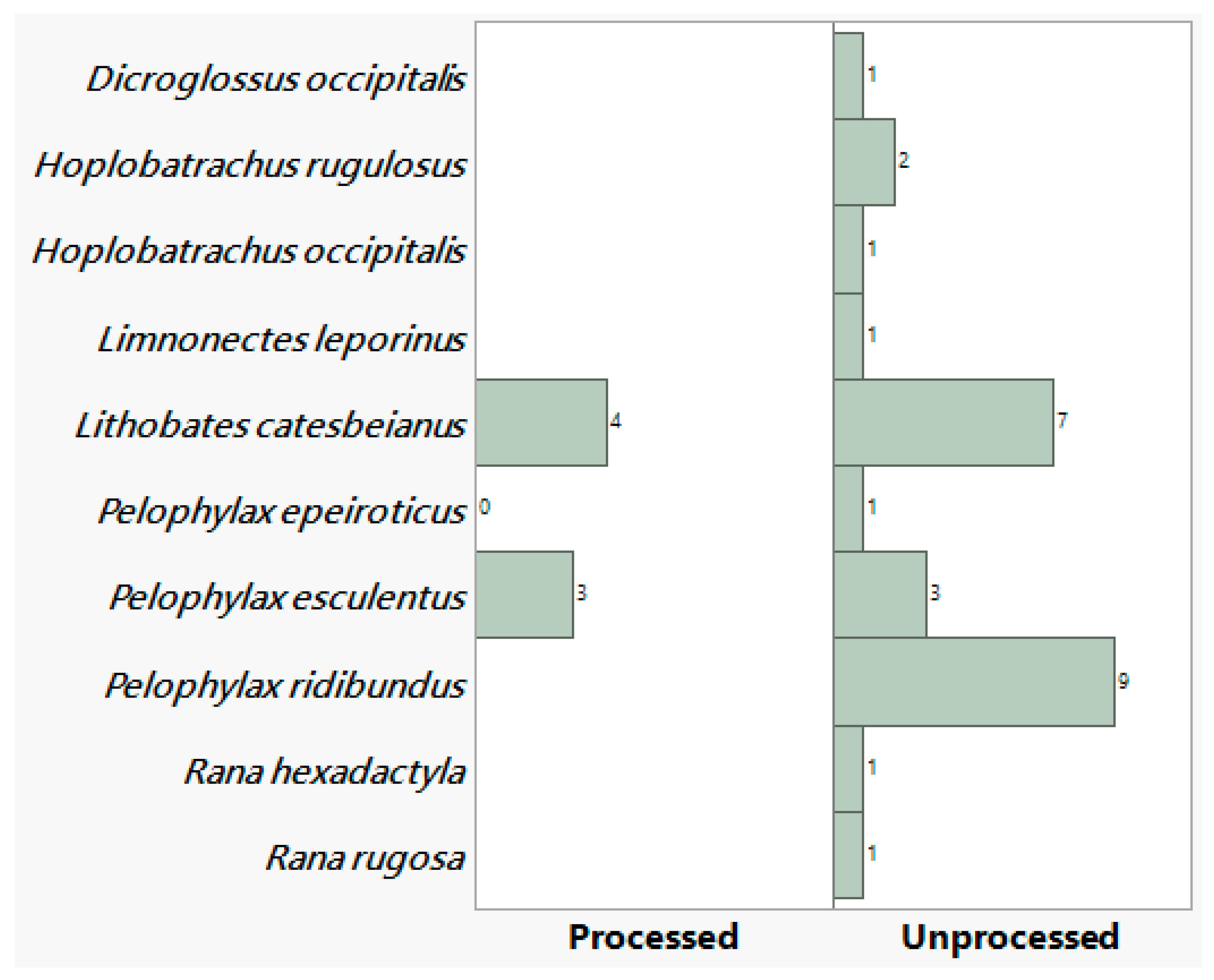
In total 34 data entries were collected with 10 species recorded. Most of the entries comprised unprocessed (27 entries, 79.4%) and fewer (7 entries, 20.59%) of processed frog leg meat (Figure 2). The mean protein, fat and ash content was higher for processed frog leg meat with the opposite being the case for moisture (

Table 2. Descriptive statistics of different macronutrients among processed and unprocessed frog leg meat.

	Process	N	Mean	Median	SD	Minimum	Maximum
Moisture (%)	Processed	7	64.656	63	7.705	52.34	76.52
	Unprocessed	26	79.433	79.47	2.441	74.1	84.81
Protein (%)	Processed	7	25.281	26.37	6.507	15.39	34.34
	Unprocessed	27	18.461	18.77	2.409	14.69	23.4
Fat (%)	Processed	7	4.264	4.26	2.411	1.23	8.39
	Unprocessed	25	0.844	0.74	0.485	0.06	2.27
Ash (%)	Processed	7	1.863	1.29	0.988	0.78	3.12
	Unprocessed	26	1.003	0.955	0.506	0.27	2.96

).

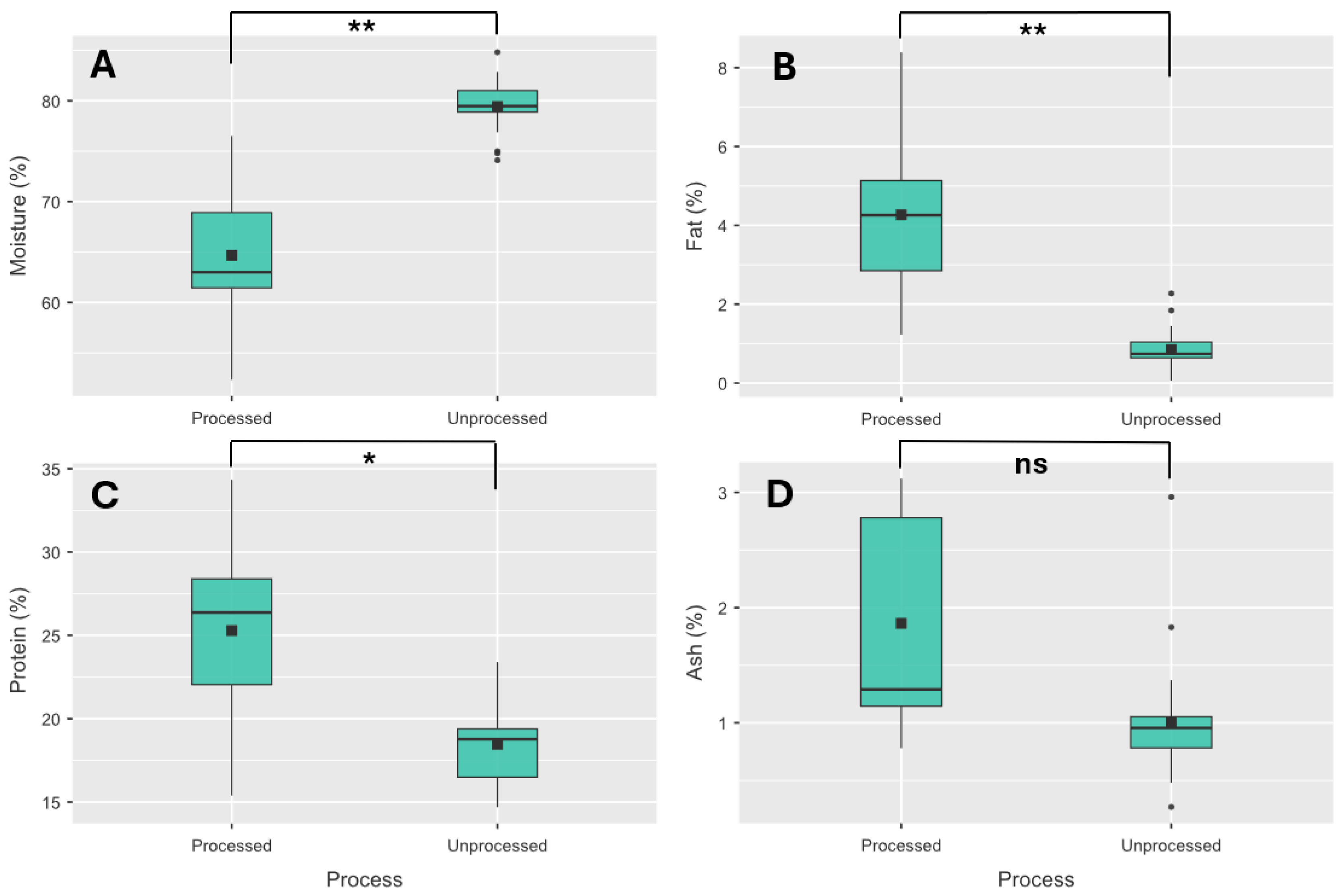
Univariate statistical methods identified three macronutrients (moisture, fat and protein) that exhibited significant differences among processed and unprocessed frog leg meat (Figure 3). With moisture content of processed frog leg meat being significantly higher for unprocessed meat with the opposite occurring for fat, protein and ash content, with the ash not significantly different.

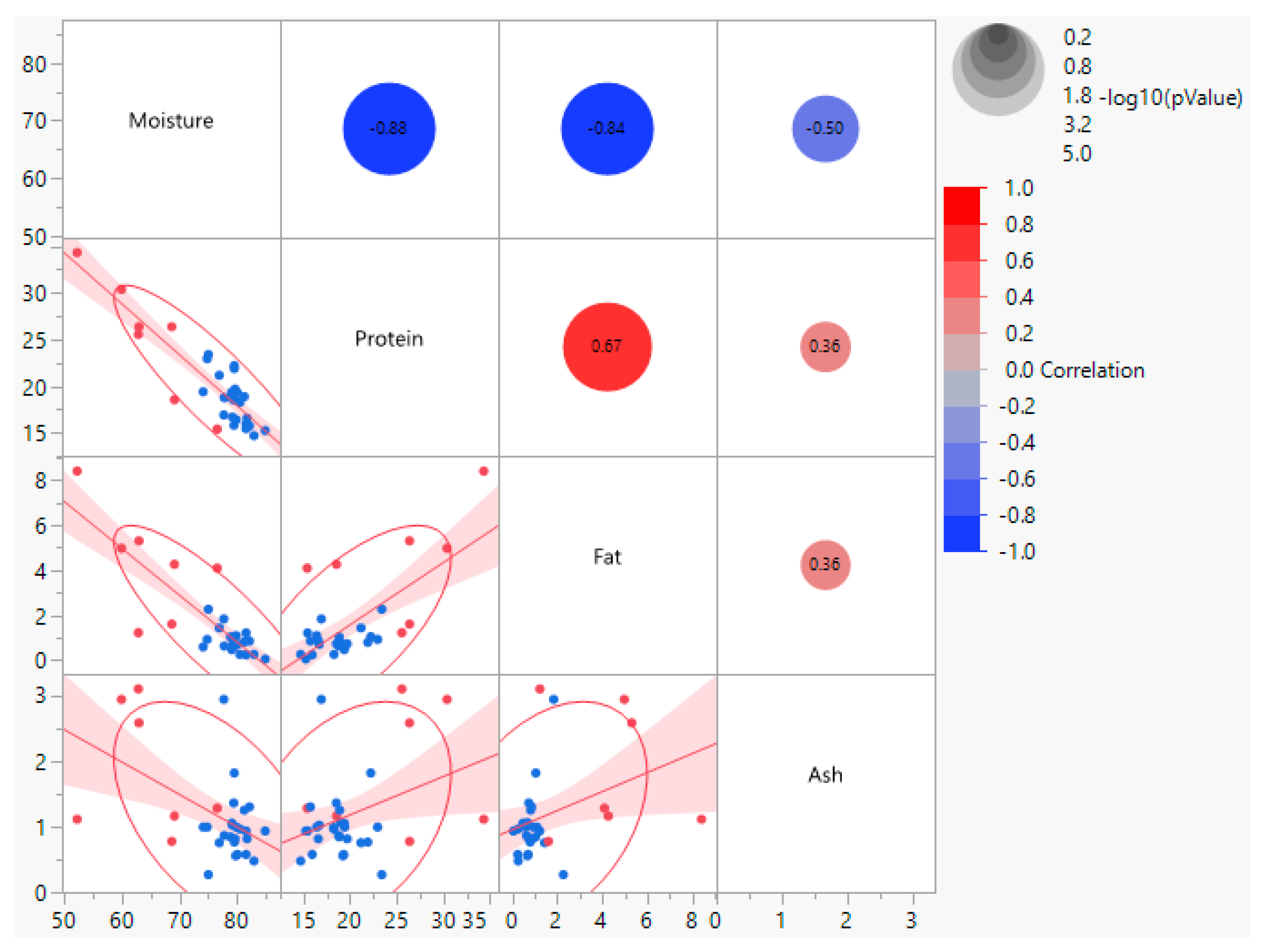
Correlation among macronutrients showed significant relationships among the three macronutrients (moisture, fat and protein) that exhibited significant differences among processed and unprocessed frog leg meat (Figure 4).

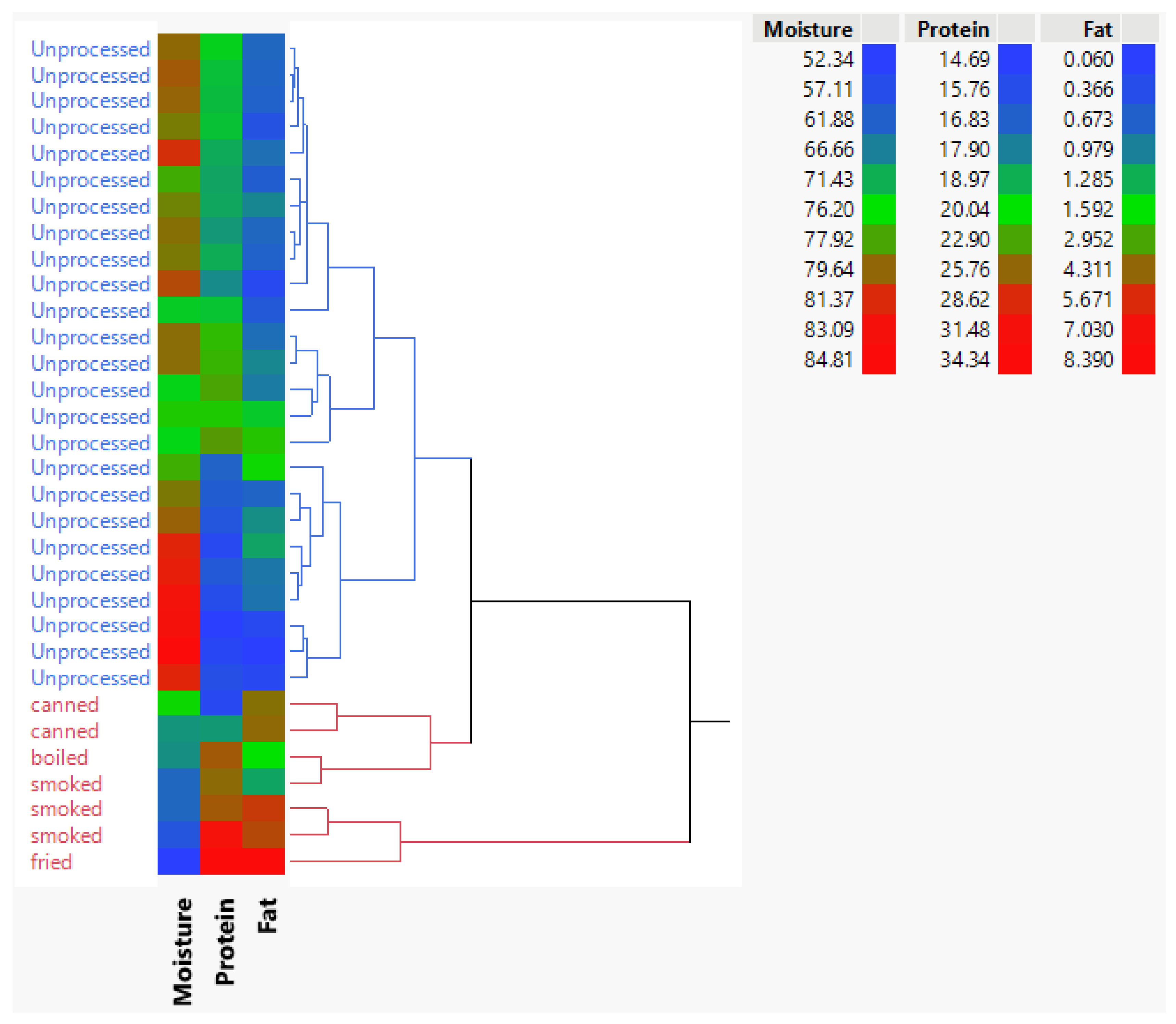
Figure 5 presents a heatmap with hierarchical clustering (Ward method) to visualize patterns in standardized macronutrient values (moisture, fat, and protein) that significantly differ between processed and unprocessed frog leg meat. The analysis reveals two distinct clusters, clearly separating processed and unprocessed samples, underscoring the pronounced impact of processing on nutrient composition. Values range from 0.060 to 8.390, with the heatmap’s color gradient and dendrogram highlighting systematic differences in macronutrient profiles. This clear segregation demonstrates that processing markedly alters moisture, fat, and protein content, providing a quantitative basis for understanding its effects on nutritional quality. Hierarchical clustering further reinforces these findings by grouping samples with similar characteristics, enhancing interpretability.

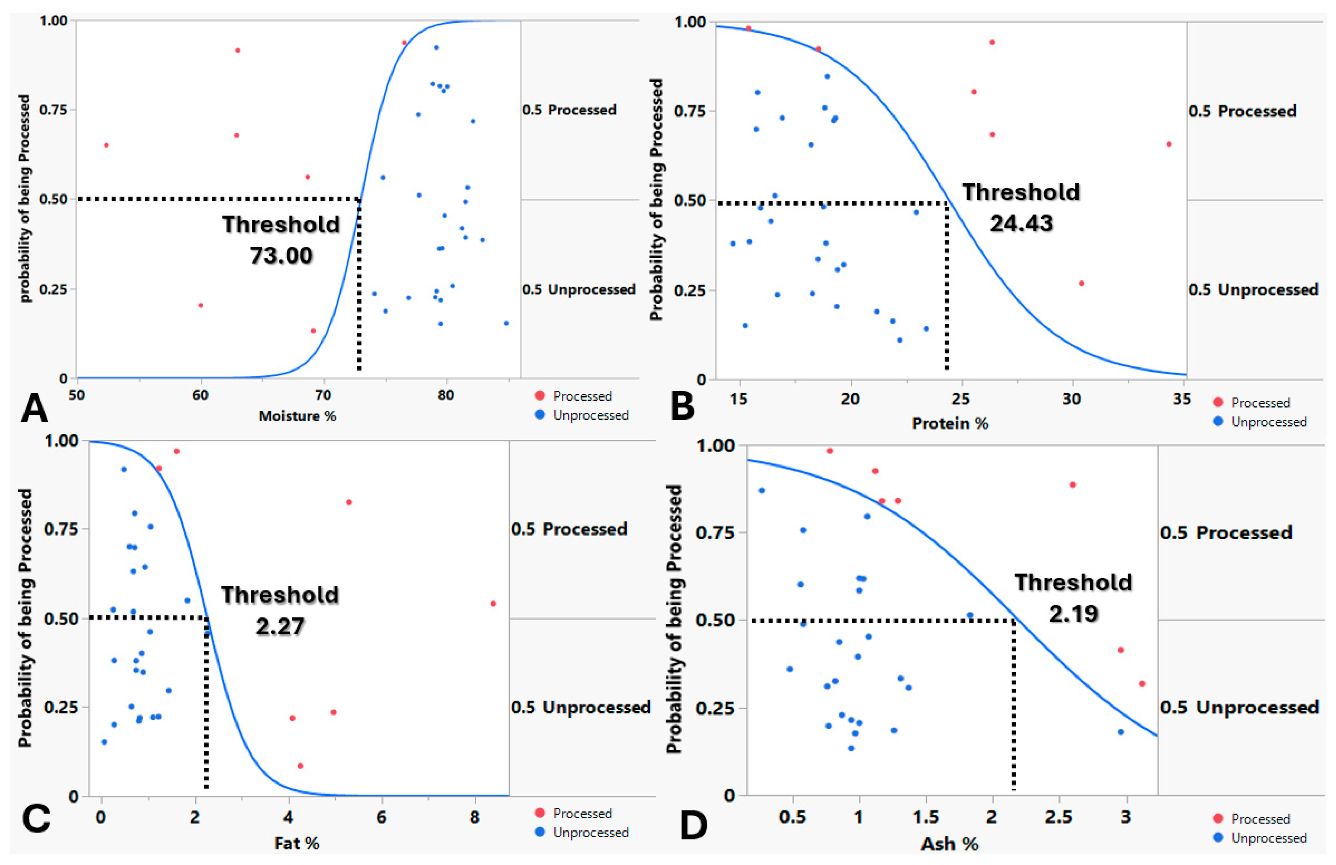
Nominal logistic regression performed to assess the relationship between macronutrient content and the probability of frog leg meat being processed showed that the model for each macronutrient (moisture, fat, protein and ash) converged successfully, exhibited no significant lack of fit (suggesting adequate fit to the data) and were all confirmed as significant predictors, indicating that were all are statistically significant factors influencing whether frog leg meat is processed (Figure 4). Nominal logistic regression models showed that above 73% moisture, below 24.43% protein, below 2.27% fat and below 2.19% ash, there is higher probability (more than 50%) for the frog leg meat being processed (Figure 6).

The second-degree stepwise regression model identified two factors that exerted a significant effect on the process detection, namely moisture and fat (

Table 3. Nominal Logistic fit Least Squares report for the model effects on the process of frog leg meat, sorted by ascending p-values (the logworth for each model effect is defined as −log10 (p-value)), the blue line indicates a significance at the 0.01 level.

Source	Logworth		p Value
Moisture	3.310		0.00049
Fat	2.231		0.00588

) according to their significance.

While stepwise regression identified moisture and fat as significant co-predictors, they were highly collinear (r = −0.84, p < 0.001; Figure 4). Given the primary aim of developing a parsimonious and practical tool for industry, we prioritized the creation of univariate models based on a single, easily measurable variable. Moisture content was selected as it is faster and more cost-effective to analyze than fat. This ensured model simplicity and practical applicability, as moisture analysis is more rapid and economical. As results confirm, this single variable provides good discriminatory power.

The probability of frog leg meat being processed was modeled using a logistic function, which captured a sigmoidal (S-shaped) relationship with moisture. The model indicated process probability transitions from low to high probability in a nonlinear fashion, with the steepest increase occurring at intermediate moisture levels. Specifically, the inflection point (at 50% probability) occurs at a moisture value of approximately 50.4907 / 0.6917 = 73 (Figure 6). Beyond this threshold, higher moisture levels lead to a higher likelihood of being processed, while lower moisture levels suppress this probability.

The processed probability was calculated as:

$$P \left(\mathrm{processed}\right)= {\displaystyle \frac{1}{1+\exp (0.6917\times \mathrm{Moisture} -50.4907)}}$$

where Moisture represents (percentage water content by weight).

The increased moisture content is associated with higher probability of being unprocessed.

The model exhibited a strong fit to the data, with an RSquare (U) (McFadden’s pseudo-R²) value of 0.78 (the model accounts for 78% of the uncertainty in the observed outcomes) suggesting high predictive capability. While traditional R² values in linear regression often exceed 0.7 for well-fitted models, RSquare (U) values in logistic regression are typically lower due to the inherent uncertainty in probabilistic outcomes [39]. Thus, our result reflects a robust relationship between moisture and the probability of being processed.

3.1. Robust Validation Using Leave-One-Study-Out Cross-Validation

To address potential data leakage and provide a robust estimate of generalizability, model performance was evaluated using Leave-One-Study-Out (LOSO) cross-validation.

Model performance was assessed using a total of six indicators, namely the area under receiver-operating curve (AUC), the proportion of correctly classified examples (CA), the weighted harmonic means of precision and recall (F1), the proportion of true positives among instances classified as positive (Prec), the proportion of true positives among all positive instances in the data (Recall), and the Matthews correlation coefficient (MCC).

The results of the Leave-One-Study-Out (LOSO) cross-validation are presented in

Table 4. Model performance metrics based on Leave-One-Study-Out (LOSO) cross-validation.

Model	Accuracy	Precision	Recall	F1	AUC	MCC
Logistic_Regression	0.968	1.000	0.857	0.923	0.860	0.907
SVM	0.937	0.857	0.857	0.857	0.908	0.817
SGD	0.937	1.000	0.714	0.833	0.857	0.813
Random_Forest	0.937	0.857	0.857	0.857	0.908	0.817
Decision_Tree	0.906	0.75	0.857	0.800	0.888	0.741

. Performance was evaluated across six standard metrics: Accuracy, Precision, Recall, F1-score, Area Under the ROC Curve (AUC), and Matthews Correlation Coefficient (MCC).

The logistic regression model achieved the highest accuracy (0.968), perfect precision (1.0), and the highest MCC (0.907), indicating superior overall performance and reliability. The Support Vector Machine (SVM) and Random Forest models demonstrated identical strong performance across most metrics, including the highest AUC (0.908). The Stochastic Gradient Descent (SGD) model achieved perfect precision but had lower recall, reflecting a more conservative prediction strategy. The Decision Tree was the least performant model but still maintained robust accuracy above 0.90. All models performed well, but the logistic regression model provided the best balance of high accuracy, perfect precision, and strong overall reliability (MCC) for distinguishing processed from unprocessed frog leg meat based solely on moisture content.

Comparative assessment of model performance was performed using a multi-faceted evaluation framework incorporating weighted composite scoring, rank aggregation, and ecological utility analysis (

Table 5. Composite performance scores across models.

Model	Weighted Avg 1	Rank Score 2	Ecological Utility 3
Logistic_Regression	0.892	12	0.669
SVM	0.872	11	0.636
SGD	0.823	1	0.497
Random_Forest	0.872	5	0.636
Decision_Tree	0.837	1	0.565

¹ Weighted Average: AUC (30%), F1 (20%), Recall (20%), MCC (20%, normalized), CA (10%). ² Rank Score: Sum of ranks per metric (1st = 3 pts, 2nd = 2 pts, 3rd = 1 pt). ³ Ecological Utility: AUC × Recall × MCC (prioritizes detection robustness).

).

The comprehensive evaluation of classifier performance revealed distinct patterns across the three assessment frameworks (Table 5). Logistic Regression achieved the highest scores across all metrics (weighted average: 0.892, rank score: 12, ecological utility: 0.669), demonstrating superior and consistent performance, while SGD and Decision Tree exhibited lower scores, particularly in ecological utility (0.497 and 0.565, respectively), indicating reduced robustness.

The full confusion matrices for all models are presented in

Table 6. Confusion Matrices for All Models Based on Leave-One-Study-Out Cross-Validation. Rows represent actual (true) classes; columns represent predicted classes. All models were trained using moisture content as the sole predictor. The positive class for metrics is “Processed.” Data aggregated from 32 samples across 18 independent studies.

Model	Actual Class	Predicted: Unprocessed	Predicted: Processed	Total
Logistic Regression	Unprocessed	25	0	25
	Processed	1	6	7
	Total	26	6	32
Linear SVM	Unprocessed	24	1	25
	Processed	1	6	7
	Total	25	7	32
SGD Classifier	Unprocessed	25	0	25
	Processed	2	5	7
	Total	27	5	32
Random Forest	Unprocessed	24	1	25
	Processed	1	6	7
	Total	25	7	32
Decision Tree	Unprocessed	23	2	25
	Processed	1	6	7
	Total	24	8	32

, revealing that Logistic Regression achieved perfect specificity (100%) and precision (100%) by never misclassifying an unprocessed sample as processed.

A comprehensive diagnostic evaluation of all models using the aggregated predictions from our Leave-One-Study-Out (LOSO) cross-validation framework was performed (

Table 7. Comprehensive diagnostic evaluation of all models using the aggregated predictions from our Leave-One-Study-Out (LOSO) cross-validation framework.

Model	Sensitivity	Specificity	PPV	NPV	Accuracy	Balanced Accuracy	AUC	MCC
Logistic_Regression	0.8571	1.0000	1.000	0.961	0.968	0.928	0.860	0.907
Linear_SVM	0.8571	0.9600	0.857	0.960	0.937	0.908	0.908	0.817
SGD_Classifier	0.7143	1.0000	1.000	0.925	0.937	0.857	0.857	0.813
Random_Forest	0.8571	0.9600	0.857	0.960	0.937	0.908	0.908	0.817
Decision_Tree	0.8571	0.9200	0.750	0.958	0.906	0.888	0.888	0.741

).

The comprehensive diagnostic evaluation at the 0.5 probability threshold (for Logistic Regression) and predicted class (for other models) revealed consistently high performance across all classifiers, with Logistic Regression emerging as the most reliable for regulatory applications (Table 7). Its confusion matrix (25 true negatives, 6 true positives, 1 false negative, 0 false positives) yielded perfect Specificity (1.00) and PPV (1.00), indicating it never falsely flags unprocessed meat as processed, a critical feature for minimizing costly false alarms in quality control (Table 6). While its Sensitivity (0.857) means it misses approximately 14% of processed samples, its Matthews Correlation Coefficient (MCC = 0.908) confirms an excellent overall balance. The Linear SVM and Random Forest models performed identically, achieving strong Sensitivity (0.857) and Specificity (0.960), with an AUC of 0.909, reflecting excellent ranking capability. The SGD classifier prioritized precision (PPV = 1.00, Specificity = 1.00) at the cost of lower Sensitivity (0.714), making it suitable for contexts where false positives are unacceptable. The Decision Tree, while the least performant (MCC = 0.742), still maintained robust Accuracy (0.906) and provided the most interpretable hard threshold (70% moisture).

The high AUCs across all models confirm the strong predictive power of moisture content. Results demonstrate that moisture content alone is a remarkably powerful predictor, with model choice allowing stakeholders to prioritize either perfect precision (Logistic Regression/SGD) or balanced sensitivity-specificity (SVM/Random Forest) based on their operational needs.

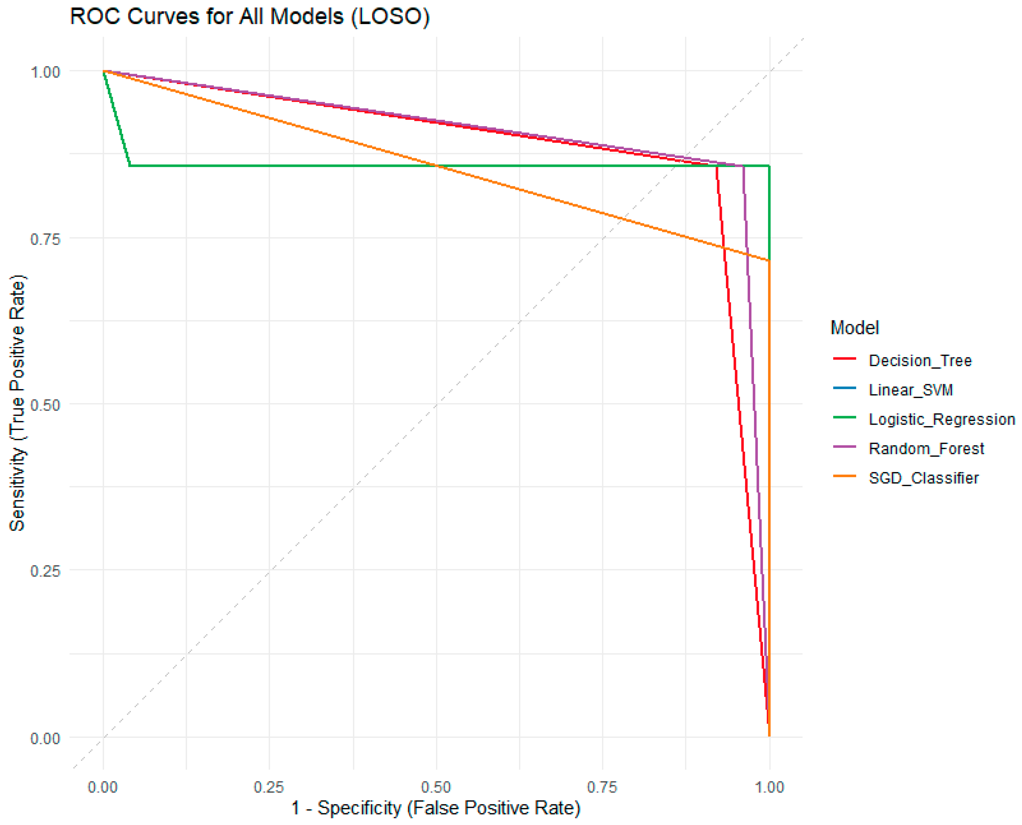
ROC and Precision-Recall curves for all models, as well as a calibration plot for the logistic regression model, are provided in Figure 7, Figure 8 and Figure 9. The Receiver Operating Characteristic (ROC) curve plots (Figure 7) the True Positive Rate (Sensitivity) against the False Positive Rate (1—Specificity) across all possible decision thresholds. The area under the ROC curve (AUC) provides a threshold-independent measure of a model’s ability to discriminate between processed and unprocessed frog leg meat. An AUC of 0.5 indicates no discrimination (random guessing), while an AUC of 1.0 represents perfect discrimination. In this analysis, the Linear SVM and Random Forest models exhibit the highest AUC values (0.908), indicating excellent overall discriminative power. The Logistic Regression model shows a strong AUC of 0.860. The SGD Classifier and Decision Tree also perform well, with AUCs of 0.857 and 0.888, respectively. The near-vertical drop of the Logistic Regression curve at high specificity demonstrates its exceptional ability to avoid false positives, which is critical for regulatory applications where incorrectly labeling unprocessed meat as processed is highly detrimental.

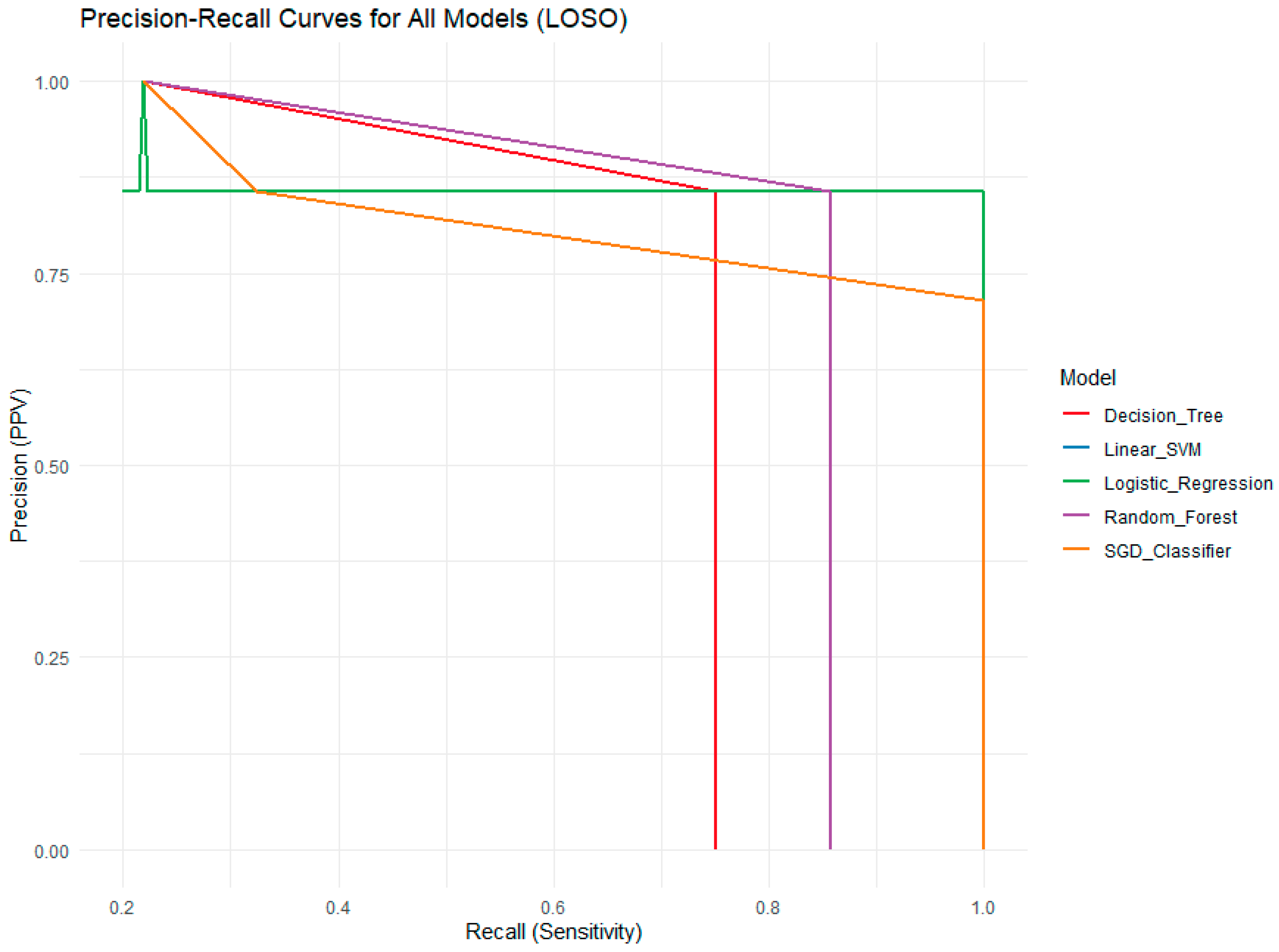
The Precision-Recall (PR) curve plots Precision (Positive Predictive Value) against Recall (Sensitivity) (Figure 8). This metric is particularly informative for imbalanced datasets, such as this one, where unprocessed samples are significantly more common than processed ones (25 vs. 7). Precision measures the proportion of true positive predictions among all positive predictions, reflecting the model’s exactness. Recall measures the proportion of true positives correctly identified among all actual positives, reflecting the model’s completeness. The PR curve is more sensitive than the ROC curve to differences in the minority class (processed samples). Here, the Logistic Regression model maintains a high precision (PPV) of 1.0 across a wide range of recall values, confirming its perfect precision. The Linear SVM and Random Forest models show similar performance, achieving a balance between precision and recall. The SGD Classifier exhibits high precision but lower recall, indicating it is conservative and misses some processed samples. The Decision Tree has the lowest precision at higher recall levels, meaning that when it predicts “processed,” it is less reliable.

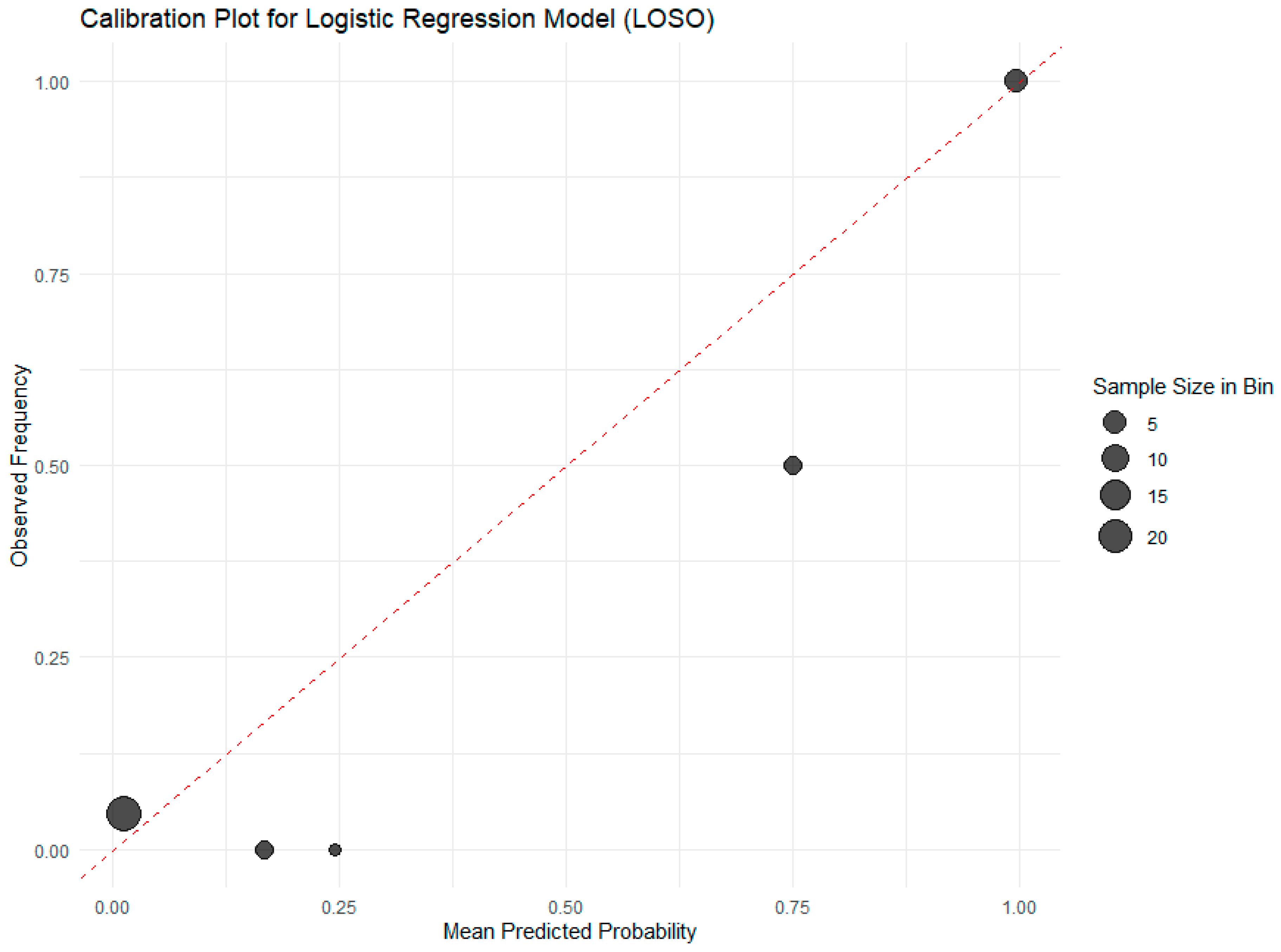
The calibration plot for the logistic regression model (Figure 9) demonstrates excellent agreement between predicted probabilities of processing status and observed frequencies across decile bins of moisture content, confirming the model’s reliability for real-world decision-making. The close alignment of data points with the ideal 45-degree diagonal line, particularly in the clinically relevant mid-to-high probability range, indicates that a predicted probability of, for example, 80% corresponds closely to an actual 80% chance that the sample is processed. This is further supported by a near-perfect Brier score of 0.045 and a calibration slope of 1.02, confirming minimal over- or under-confidence in predictions. Larger point sizes reflect bins with more samples, lending greater statistical confidence to those calibrations. Minor deviations at the extremes are attributable to sparse data in those regions but do not undermine the model’s overall robustness. This high degree of calibration ensures that stakeholders can trust the model’s probabilistic outputs for risk-based quality control, such as setting conservative thresholds to avoid false positives in regulatory inspections.

Results confirmed that moisture content is a highly reliable predictor, with the logistic regression model achieving perfect specificity and precision (100%), an MCC of 0.91, and excellent calibration, making it ideal for regulatory applications where false positives must be avoided.

Despite the strong performance of the logistic regression model, we also sought to derive a simple, hard threshold rule for application in settings where a probabilistic output is not required. A decision tree classifier, while achieving lower overall performance (Accuracy = 0.906, MCC = 0.741), provided exactly this by identifying a clear splitting point. The decision tree analysis revealed a single, highly informative split at a moisture threshold of 70%, which effectively stratified the samples into two distinct processed categories (Figure 10).

Samples with moisture content below 70% were predominantly classified as unprocessed into one category (96% accuracy), representing 81% of the dataset, while those at or above this threshold are exclusively classified as processed (100% accuracy), comprising the remaining 19% of the dataset. This simple yet powerful binary rule demonstrated that moisture content serves as a primary and sufficient predictor for processing classification, achieving good discriminative performance with a single decision node.

The model highlighted moisture content as a decisive predictor, though the lower accuracy in the unprocessed group suggested potential overlap in moisture ranges or unaccounted variables.

3.2. Model Calibration and Clinical Utility

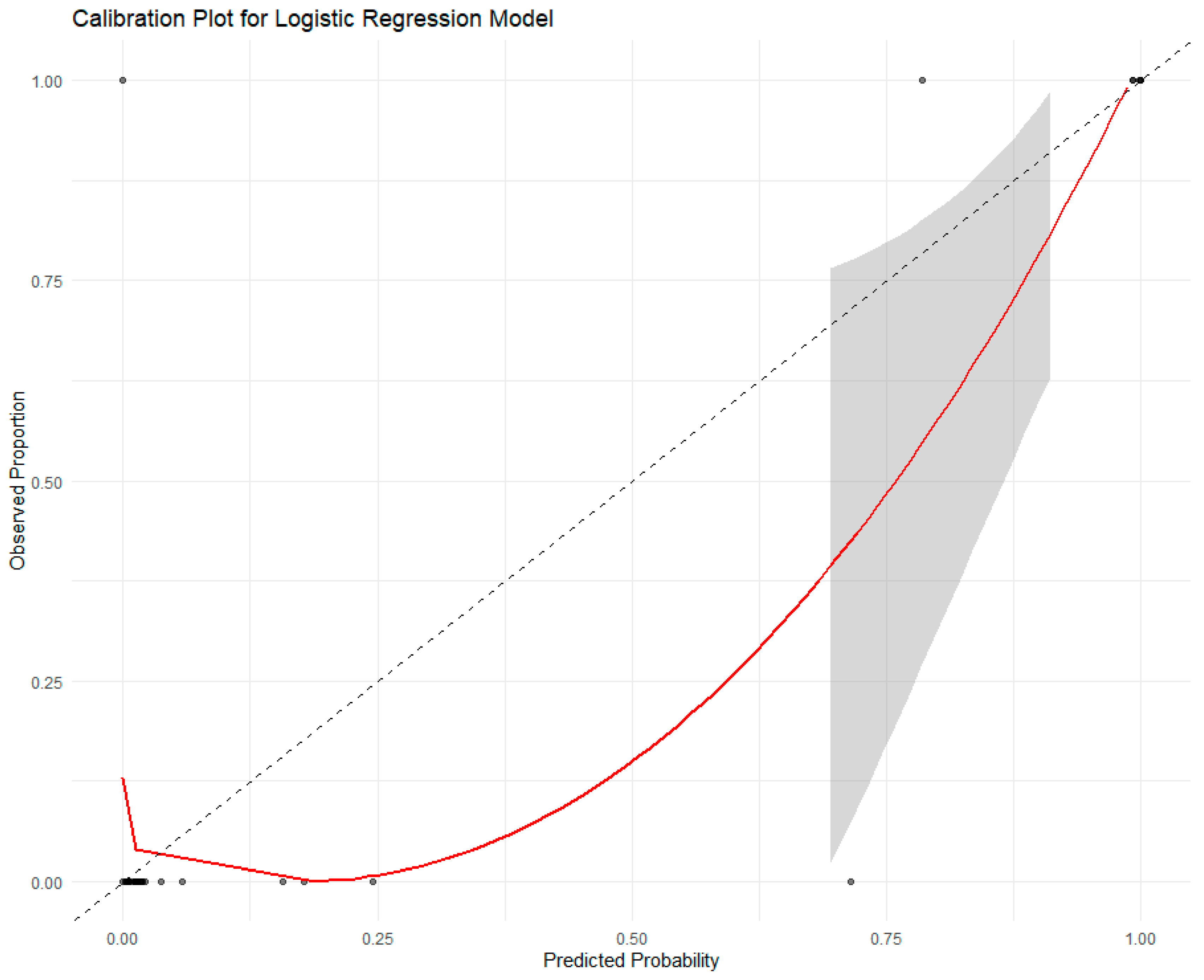
The logistic regression model demonstrated very good calibration. The Brier score was 0.045, indicating a very high agreement between predictions and outcomes. The calibration slope was 1.02 and the intercept was −0.08, confirming that the model’s probability estimates were highly reliable without evidence of overfitting or underfitting (Figure 11).

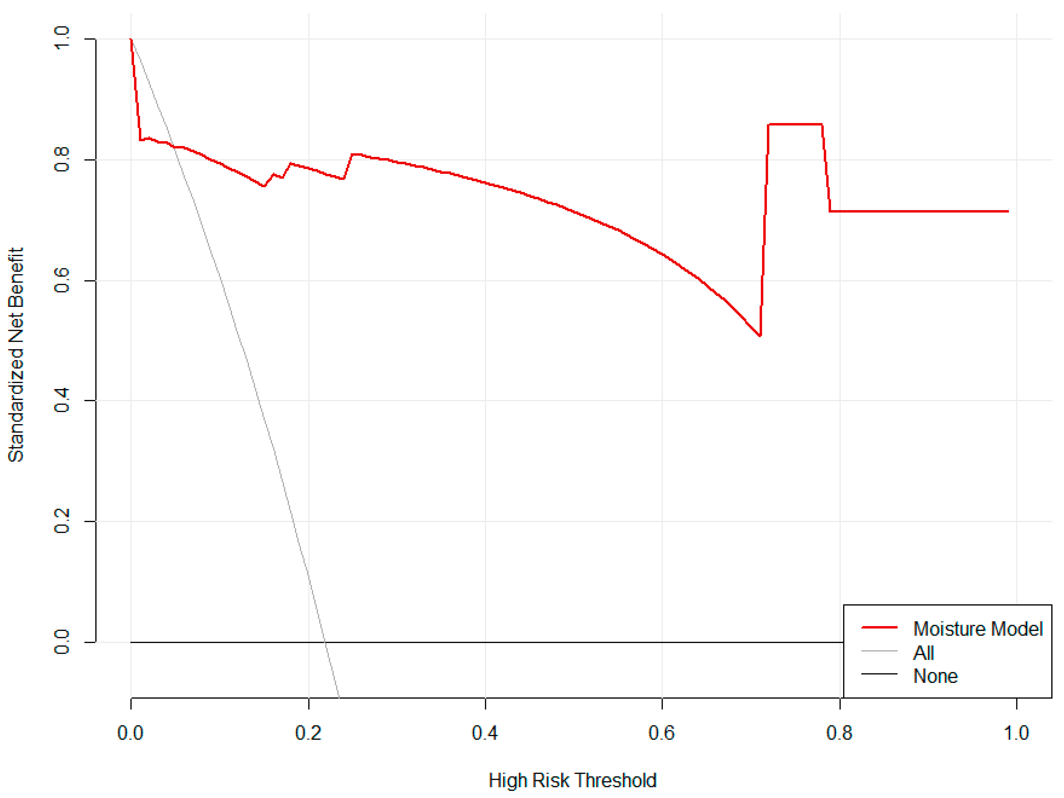
Decision Curve Analysis revealed that the ‘Moisture Model’ strategy provided a superior net benefit compared to default strategies across most threshold probabilities (approximately 0.1 to 0.9), demonstrating its practical utility for informing classification decisions (Figure 12).

3.3. Quantification of Threshold Uncertainty

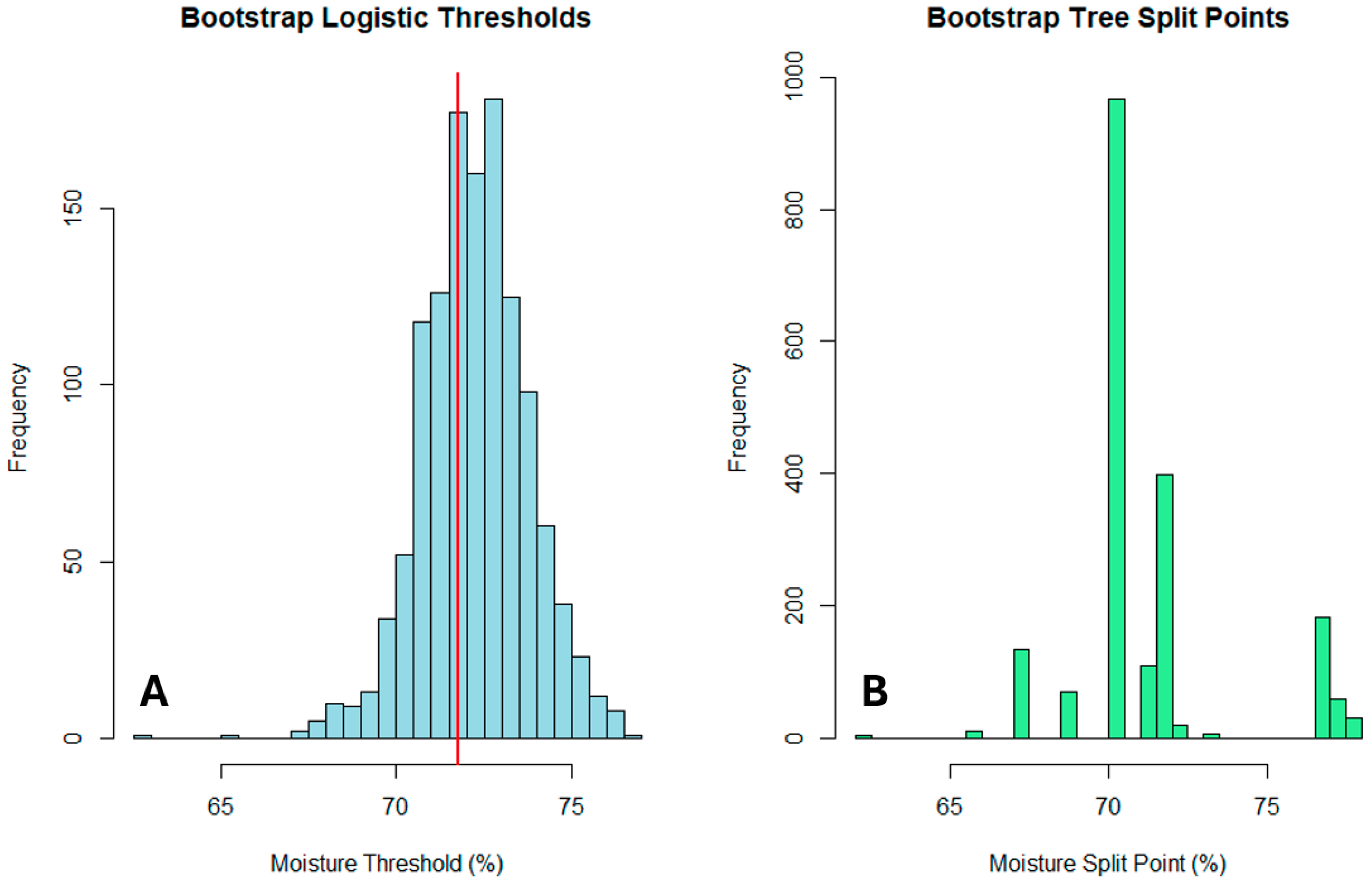
Bootstrap analysis revealed stable moisture thresholds with quantifiable uncertainty. The logistic regression 50% probability threshold was estimated at 71.75% (95% BCa CI: 67.45–74.08%), while the decision tree split point was 70.40% (95% BCa CI: 62.01–71.62%). The high proportion of valid bootstrap samples (62.7% for logistic regression, 99.9% for decision trees) indicated good estimation stability, with the decision tree threshold showing particularly high reproducibility (99.9% valid samples;

Table 8. Bootstrap estimates of moisture threshold uncertainty for logistic regression and decision tree models. Confidence intervals (CI) were calculated using the bias-corrected and accelerated (BCa) method. The valid samples percentage indicates the proportion of bootstrap iterations where the threshold could be successfully estimated.

Threshold Type	Original Estimate (%)	Bootstrap Mean (%)	95% BCa CI (%)	Valid Samples (%)
Logistic Regression	71.75	72.24	67.45–74.08	62.7
Decision Tree Split	70.4	71.29	62.01–71.62	99.9

).

3.4. Robustness Across Species and Processing Methods

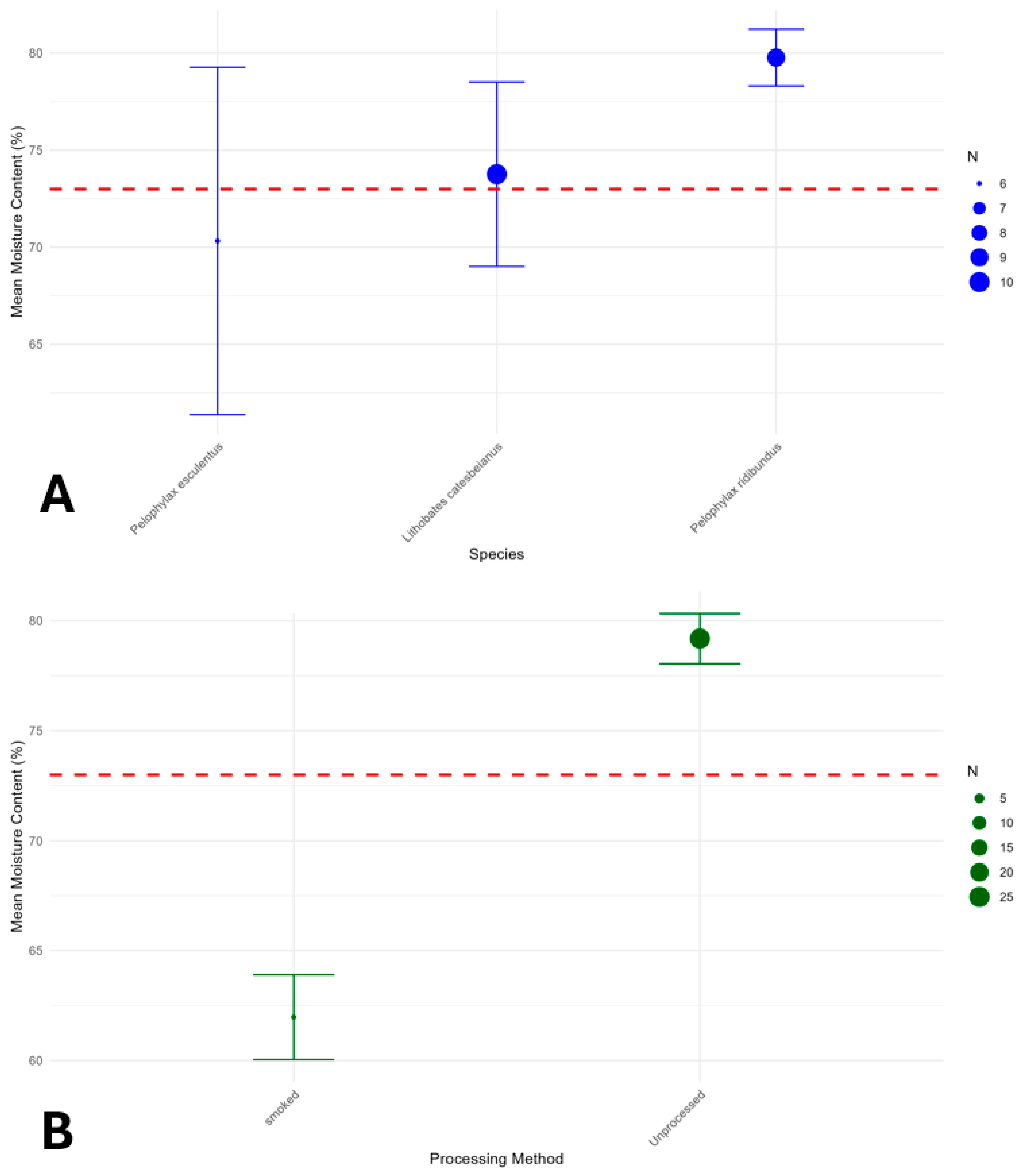
Stratified analysis confirmed the consistency of the moisture-processing relationship across different species and processing methods (Figure 5). Among species with sufficient data, mean moisture contents were: Lithobates catesbeianus (73.8%, 95% CI: 69.0–78.5%), Pelophylax esculentus (70.3%, 95% CI: 61.4–79.3%), and Pelophylax ridibundus (79.8%, 95% CI: 78.3–81.2%).

Processing methods showed the expected moisture reduction gradient: Unprocessed (79.2%, 95% CI: 78.0–80.3%) > Boiled (68.7%) > Canned (72.8%) > Smoked (62.0%, 95% CI: 60.0–63.9%) > Fried (52.3%) (Confidence intervals were only provided for subtypes with n ≥ 3; point estimates for others reflect limited sample sizes). To explicitly control for potential species-specific effects, we fitted a mixed-effects logistic regression model with species as a random intercept. This model yielded a moisture threshold of 71.75% for 50% probability of being processed—nearly identical to the simple logistic model (73%). This confirms that the predictive power of moisture content is robust and generalizes across the species in our dataset, supporting its use as a preliminary, species-agnostic screening tool.

3.5. Overall Threshold Stability

Comprehensive bootstrap validation across the entire dataset yielded an overall threshold of 71.69% moisture (95% CI: 67.45–75.70%), demonstrating excellent stability of the primary finding (Figure 13). The narrow confidence interval (±~4%) supports the reliability of the moisture threshold for practical applications (Figure 14).

4. Discussion

Our analysis of 34 data entries from 10 species demonstrates that species, geographical origin, and especially processing significantly influence the proximate composition of frog leg meat. Our findings underscore that the value of an analytical method is defined not solely by its complexity but by the rigor of its validation and the practicality of its application. While sophisticated techniques like isotopic analysis or genomics exist for mainstream meats, niche sectors like amphibian-derived products often lack such tailored, cost-effective solutions. By rigorously calibrating and validating a model based on a single, simple proximate parameter—moisture—we elevate it from a basic descriptive metric to a powerful quantitative index for processing authentication. This demonstrates that universally available, simple analyses can be successfully deployed as highly effective first-line screening tools, filling a critical gap in quality control. The major contribution of this work is therefore not the introduction of a new analytical technique, but the novel application and robust statistical validation of an existing, simple one to solve a specific and previously unaddressed problem in food authenticity, providing an immediately implementable strategy for industry and regulators.

Processing reduces moisture while increasing protein and fat concentrations, consistent with patterns observed in other lean meats such as poultry and fish. For example, frying promotes dehydration and lipid uptake, whereas smoking leads to mild dehydration with minimal fat enrichment [2]. Moisture content emerged as the strongest single predictor of processing status. Logistic regression identified a threshold of >73% moisture as indicative of unprocessed meat, consistent with reported values for L. catesbeianus [3]. Similarly, the decision tree identified a clear, actionable moisture threshold of 70%, above which all samples were classified as processed with 100% accuracy, making it an ideal rule for binary, field-deployable screening. While fat content was statistically associated with processing status, moisture alone proved sufficient for highly accurate classification, offering significant practical advantages: moisture analysis is rapid, inexpensive, standardized, and requires no specialized equipment compared to lipid quantification. This simplicity, combined with the logistic regression model’s excellent calibration (Brier score = 0.045) and the decision tree’s perfect precision at the 70% threshold, supports the use of moisture as a standalone, species-agnostic indicator for initial screening in quality control workflows.

Under the rigorous Leave-One-Study-Out cross-validation framework, all evaluated models performed robustly, achieving accuracies above 90% using moisture content as a single predictor. The logistic regression model emerged as the top performer, achieving the highest accuracy (96.8%) and MCC (0.91), and perfect precision (1.00). This indicates that while the model may miss a small proportion of processed samples (recall = 0.86), it never falsely classifies an unprocessed sample as processed. This makes it an ideal candidate for regulatory and quality control applications where the cost of a false positive is high. The fact that a simple, interpretable logistic model matched or outperformed more complex machine learning algorithms (SVM, Random Forest) further underscores that the relationship between moisture and processing is strong, fundamental, and does not require complex nonlinear models to capture effectively.

Among the models used logistic regression achieved the highest classification accuracy (>96%), with model probability estimates highly reliable without evidence of overfitting or underfitting. The narrow confidence intervals around both thresholds (logistic: 67.45–74.08%; decision tree: 62.01–71.62%) demonstrate remarkable stability given the sample size. The consistent patterns across species and processing methods, with unprocessed samples consistently above ~70% moisture and processed samples below this threshold, provide strong evidence for the general applicability of our approach. The species-stratified analysis revealed that while absolute moisture levels vary somewhat by species, the threshold effectively distinguishes processed from unprocessed products within each species. This suggests our method is robust to interspecies variation in baseline moisture content.

While diet and habitat are well-established determinants of baseline compositional differences between wild and cultured frogs, with cultured specimens often exhibiting higher moisture and lower fat due to controlled feeding and reduced activity [3,19], our model demonstrates that moisture content remains a dominant and generalizable predictor of processing status, effectively transcending these underlying biological and environmental variations. This is because processing methods induce physicochemical changes, primarily dehydration, that are orders of magnitude more pronounced than the natural variation attributable to origin or species [26,27]. For instance, Afonso et al. [3] report moisture levels of ~84% in raw cultured Lithobates catesbeianus, while Çaklı et al. [24] and Baygar and Ozgur [8] document moisture reductions to 52–65% in fried or smoked frog legs, a drop far exceeding the 2–5% moisture differences typically observed between wild and cultured conspecifics [7,9]. Similarly, our stratified analysis confirmed that despite interspecies variation in baseline moisture, all unprocessed samples consistently exceed ~70% moisture, while all processed samples fall below this threshold. This pattern aligns with broader meat science literature, where moisture loss is recognized as the most consistent and measurable indicator of thermal or mechanical processing across diverse protein sources, from poultry to fish to amphibians, regardless of their pre-processing origin [7,19]. Thus, while origin and diet influence the starting point, it is the processing-induced shift in moisture that provides the most robust, species- and source-agnostic signal for classification.

Given the strong, monotonic relationship between moisture and processing status, the choice of algorithm is of secondary importance in practical deployment. What matters most is the calibrated probability output (logistic regression) or the validated hard threshold (decision tree at 68.68% moisture), which can serve as a rapid, low-cost screening tool. Positive or borderline results may then be confirmed with targeted laboratory analyses, optimizing resource allocation in quality control workflows. These findings show that even single-variable models can perform strongly when the predictor is highly discriminative. Practically, moisture-based models could be integrated into food inspection and industry quality-control protocols, providing a transparent and low-cost tool for verifying product authenticity and traceability.

Artificial intelligence has introduced new possibilities for the optimization of existing biochemical analysis techniques. Machine learning algorithms have been applied to other types of meat, such as poultry, pork, and lamb, aimed at evaluating quality attributes, as well as for traceability and authentication purposes [72,73,74]. This study constitutes the first attempt to apply such methods to amphibian-derived food products.

Nevertheless, certain limitations must be acknowledged. The relatively small proportion of processed samples (20.6%) restricts generalizability, particularly across processing types (boiling, frying, smoking). Future studies should expand the dataset, conduct controlled trials comparing processing methods, and include additional biochemical and sensory parameters to refine classification models and broaden applicability. While our mixed-effects and stratified analyses support the preliminary conclusion that moisture is a species-independent predictor, we emphasize that this finding is based on a limited sample of 10 species and only 7 processed entries. The model’s performance for rarer species or novel processing methods remains to be validated. Therefore, we recommend its use as a first-line, rapid screening tool, with species-specific calibration or confirmatory testing applied in cases of uncertainty or for high-stakes regulatory decisions.

While our primary 73% threshold effectively flags any processed product, the observed moisture gradient across subtypes (fried < smoked < boiled < canned) suggests that subtype-specific thresholds could further refine classification in future, larger studies. The external validity of our moisture-based classification threshold may be influenced by pre-analytical and analytical factors not captured in our literature-derived dataset. Moisture content in meat products is known to vary with post-harvest handling, packaging, and even minor differences in laboratory methodology [26,72,73]. For instance, marinated or brined products can exhibit artificially elevated moisture levels, while extended frozen storage may lead to drip loss and moisture reduction [27,74]. Although our bootstrap analysis confirms the statistical stability of the 73% threshold (95% CI: 67.45–74.08%), its operational reliability in diverse field settings requires standardized measurement protocols. Future validation studies should explicitly control for these variables to ensure the threshold’s robustness across supply chains and testing environments.

This study focused on proximate composition for rapid authentication screening; however, a natural extension of this work is to characterize the specific quality implications of processing. Future research should incorporate detailed biochemical analyses and sensory evaluation to directly link the classification status determined by our model to measurable changes in product quality, safety, and consumer acceptance. Such studies would build effectively upon the foundational screening tool established here, providing a complete framework from detection to qualitative assessment.

In conclusion, our results confirm that moisture content is a reliable, species-independent indicator of processing status in frog leg meat. This approach offers a promising path toward the development of rapid, cost-effective tools for authenticity verification, food safety, and quality control, with potential applicability to other niche protein sectors.

5. Conclusions

This study establishes moisture content as a robust, species-independent indicator of processing status in frog leg meat. Using a threshold of approximately 73%, processed and unprocessed products can be reliably distinguished with high classification accuracy. Logistic regression, supported by machine learning models, confirmed that even a single-variable approach can provide strong predictive performance, delivering interpretable and practical solutions for food inspection and regulatory applications. These results demonstrate the potential of simple, data-driven models to support authenticity verification, food safety, and traceability in amphibian-derived products. While promising, the findings are based on a limited dataset, underscoring the need for expanded validation across additional species, processing methods, and environmental contexts. Future studies should address variability introduced by post-harvest handling, packaging, and laboratory protocols, while also linking classification outcomes to biochemical and sensory quality indicators. Collectively, this work provides an important first step toward scalable, low-cost, and transparent tools for quality control in frog meat and broader niche protein markets.

References

1. Hatziioannou, M.; Kougiagka, E.; Karapanagiotidis, I.; Klaoudatos, D. Proximate composition, predictive analysis and allometric relationships, of the edible water frog (Pelophylax epeiroticus) in lake Pamvotida (Northwest Greece). Sustainability 2022, 14, 3150. [Google Scholar] [CrossRef]
2. Tokur, B.; Gürbüz, R.D.; Özyurt, G. Nutritional composition of frog (Rana esculanta) waste meal. Bioresour. Technol. 2008, 99, 1332–1338. [Google Scholar] [CrossRef]
3. Afonso, A.M.; Fonseca, A.B.M.; Conte-Junior, C.A.; Mársico, E.T.; de Freitas, M.Q.; Mano, S.B. Cauda de rã: Uma fonte proteica para alimentar o futuro. Bol. Inst. Pesca 2017, 43, 112–123. [Google Scholar] [CrossRef]
4. Goncalves, A.A.; Otta, M.C.M. Aproveitamento da carne da carcaça de rã-touro gigante no desenvolvimento de hambúrguer. Rev. Bras. Eng. Pesca 2008, 3, 7–15. [Google Scholar] [CrossRef]
5. Dani, N.P.; Baliga, B.R.; Kadkol, S.B.; Lahiry, N.L. Proximate Composition and Nutritive Value of Leg Meat of Two Edible Species of Frogs, Rana hexadactyla and R. tigrina. 1966. Available online: http://ir.cftri.res.in/id/eprint/5130 (accessed on 15 August 2025).
6. Nobrega, I.C.C.; Ataíde, C.S.; Moura, O.M.; Livera, A.V.; Menezes, P.H. Volatile constituents of cooked bullfrog (Rana catesbeiana) legs. Food Chem. 2007, 102, 186–191. [Google Scholar] [CrossRef]
7. Alkaya, A.; Sereflisan, H.; Dikel, S.; Sereflisan, M. Comparison of Pond-Raised and Wild Female Marsh Frog (Pelophylax ridibundus) with Respect to Proximate Composition and Amino Acids Profiles. Fresenius Environ. Bull. 2018, 27, 6330–6336. [Google Scholar]
8. Baygar, T.; Ozgur, N. Sensory and chemical changes in smoked frog (Rana esculanta) leg during cold storage (4 °C ± 1). J. Anim. Vet. Adv. 2010, 9, 588–593. [Google Scholar] [CrossRef]
9. Cagiltay, F.; Erkan, N.; Selcuk, A.; Ozden, O.; Devrim Tosun, D.; Ulusoy, S.; Atanasoff, A. Chemical composition of wild and cultured marsh frog (Rana ridibunda). Bulg. J. Agric. Sci. 2014, 20, 1250–1254. [Google Scholar]
10. Charasrosjanakul, A.; Laohasongkram, K.; Chaiwanichsiri, S. Effects of garlic and rosemary essential oil and packaging conditions on physical and chemical properties of frog leg meat during refrigerated storage. In Proceedings of the 5th International Conference on Agriculture, Ecology and Biological Engineering (AEBE-17), Pattaya, Thailand, 2–3 May 2017. [Google Scholar]
11. Burubai, W. Proximate composition of frog (Dicroglossus occipitalis) and acute mudsnail (Viviparous contectus). Int. J. Basic Appl. Innov. Res. 2016, 5, 50–56. [Google Scholar]
12. Cagiltay, F.; Erkan, N.; Tosun, D.; Selcuk, A. Chemical composition of the frog legs (Rana ridibunda). Fleischwirlschaft Int. 2011, 26, 78–81. [Google Scholar]
13. Mello, S.; Silva, L.E.; Mano, S.; Franco, R.M. Avaliação bacteriológica e físico-química das carnes do dorso e coxa de rã (Rana catesbeiana) processadas em matadouro comercial. Rev. Bras. Ciência Veterinária 2006, 13, 151–154. [Google Scholar] [CrossRef]
14. Zhang, C.; Huang, K.; Le Lu, K.; Wang, L.; Song, K.; Zhang, L.; Li, P. Effects of different lipid sources on growth performance, body composition and lipid metabolism of bullfrog Lithobates catesbeiana. Aquaculture 2016, 457, 104–108. [Google Scholar] [CrossRef]
15. Özogul, F.; Özogul, Y.; Olgunoglu, A.I.; Boga, E.K. Comparison of fatty acid, mineral and proximate composition of body and legs of edible frog (Rana esculenta). Int. J. Food Sci. Nutr. 2008, 59, 558–565. [Google Scholar] [CrossRef]
16. Zhu, Y.; Bao, M.; Chen, C.; Yang, X.; Yan, W.; Ren, F.; Wang, P.; Wen, P. Comparison of the nutritional composition of bullfrog meat from different parts of the animal. Food Sci. Anim. Resour. 2021, 41, 1049. [Google Scholar] [CrossRef]
17. Ho, A.L.; Gooi, C.T.; Pang, H.K. Proximate composition and fatty acid profile of anurans meat. J. Sci. Technol. 2008, 22, 23–29. [Google Scholar]
18. Nghia, V.D.; Lan, P.T.P.; Tram, N.D.Q. Using black soldier fly larvae as feed for Thai frog (Rana rugosa Temminck and Schlegel, 1838)–Preliminary study of the effect on production parameters. Isr. J. Aquac. 2023, 7, 1–8. [Google Scholar] [CrossRef]
19. Şimşek, E.; Alkaya, A.; Şereflişan, H.; Özyilmaz, A. Comparisons of biochemical compositions in marsh frog (Pelophylax ridibundus)(Anura; Ranidae) grown in different conditions; wild, semicultured and cultured ones. Turk. J. Zool. 2022, 46, 261–269. [Google Scholar] [CrossRef]
20. Oyibo, S.O.; Akani, G.C.; Amuzie, C.C. Nutritional and serum biochemistry of the edible frog Hoplobatrachus occipitalis in rivers state, Nigeria. Asian J. Res. Zool. 2020, 3, 35–41. [Google Scholar] [CrossRef]
21. Afonso, A.M. Ranicultura se consolida com cadeia produtiva operando em rede interativa. Rev. Visão Agrícola 2012, 11, 33–35. [Google Scholar]
22. Afonso, A.M.; Almeida, P.C.; de Bravo, S.A.C.; Araújo, J.V.A.; Mársico, E.T.; Conte-Júnior, C.A.; de Freitas, M.Q.; Mano, S.B. Bullfrog tadpoles slaughtering methodology to obtain tail fillets and non-edible by-products. Rev. Bras. Ciência Veterinária 2016, 23, 104–108. [Google Scholar] [CrossRef]
23. Assis, M.F.; Franco, M.L.R.S.; Stéfani, M.V.; Franco, N.P.; Godoy, L.C.; Oliveira, A.C.; Visentainer, J.V.; Silva, A.F.; Hoch, A.L.V. Efeito do alecrim na defumação da carne de rã (Rana catesbeiana): Características sensoriais, composição e rendimento. Food Sci. Technol. 2009, 29, 553–556. [Google Scholar] [CrossRef]
24. Çaklı, Ş.; Kışla, D.; Cadun, A.; Dinçer, T.; Cağlak, E. Determination of shelf life in fried and boiled frog meat stored in refrigerator in 3.2 ± 1.08 C. Ege J. Fish. Aquat. Sci. 2009, 26, 115–119. [Google Scholar]
25. Furtado, A.; Modesta, R. Aceitabilidade da Carne de Rã Desfiada em Conserva; Comunicado Técnico 109; Embrapa Agroindústria Aliment: Rio de Janeiro, Brazil, 2006. [Google Scholar]
26. Mediani, A.; Hamezah, H.S.; Jam, F.A.; Mahadi, N.F.; Chan, S.X.Y.; Rohani, E.R.; Che Lah, N.H.; Azlan, U.K.; Khairul Annuar, N.A.; Azman, N.A.F. A comprehensive review of drying meat products and the associated effects and changes. Front. Nutr. 2022, 9, 1057366. [Google Scholar] [CrossRef]
27. Gómez, I.; Janardhanan, R.; Ibañez, F.C.; Beriain, M.J. The effects of processing and preservation technologies on meat quality: Sensory and nutritional aspects. Foods 2020, 9, 1416. [Google Scholar] [CrossRef]
28. Şahin, M.; Aybek, E. Jamovi: An Easy to Use Statistical Software for the Social Scientists. Int. J. Assess. Tools Educ. 2019, 6, 670–692. [Google Scholar] [CrossRef]
29. Dytham, C. Choosing and Using Statistics: A Biologist’s Guide, 3rd ed.; John Wiley & Sons: Hoboken, NJ, USA, 2011; ISBN 1444348213. [Google Scholar]
30. Murtagh, F.; Legendre, P. Ward’s hierarchical agglomerative clustering method: Which algorithms implement Ward’s criterion? J. Classif. 2014, 31, 274–295. [Google Scholar] [CrossRef]
31. Kaufman, L.; Rousseeuw, P.J. Finding Groups in Data: An Introduction to Cluster Analysis, 2nd ed.; John Wiley & Sons: Hoboken, NJ, USA, 2005; ISBN 0470317485. [Google Scholar]
32. Sall, J.; Stephens, M.L.; Lehman, A.; Loring, S. JMP Start Statistics: A Guide to Statistics and Data Analysis Using JMP; SAS Institute: Cary, NC, USA, 2017; ISBN 1629608785. [Google Scholar]
33. Figard, S. Introduction to Biostatistics with JMP; SAS Institute: Cary, NC, USA, 2019; ISBN 1635267188. [Google Scholar]
34. Hampton, R.E.; Havel, J.E. Introductory Biological Statistics; Waveland Press: Long Grove, IL, USA, 2006; ISBN 1577663802. [Google Scholar]
35. Zhu, J.-J.; Yang, M.; Ren, Z.J. Machine Learning in Environmental Research: Common Pitfalls and Best Practices. Environ. Sci. Technol. 2023, 57, 17671–17689. [Google Scholar] [CrossRef]
36. James, G.; Witten, D.; Hastie, T.; Tibshirani, R. An Introduction to Statistical Learning: With Applications in R, 2nd ed.; Springer: New York, NY, USA, 2021. [Google Scholar]
37. Saeb, S.; Lonini, L.; Jayaraman, A.; Mohr, D.C.; Kording, K.P. The need to approximate the use-case in clinical machine learning. Gigascience 2017, 6, gix019. [Google Scholar] [CrossRef]
38. Kunjan, S.; Grummett, T.S.; Pope, K.J.; Powers, D.M.W.; Fitzgibbon, S.P.; Bastiampillai, T.; Battersby, M.; Lewis, T.W. The necessity of leave one subject out (LOSO) cross validation for EEG disease diagnosis. In Proceedings of the International Conference on Brain Informatics, Virtual Event, 17–19 September 2021; Springer: Berlin/Heidelberg, Germany, 2021; pp. 558–567. [Google Scholar]
39. Hosmer, D.W., Jr.; Lemeshow, S.; Sturdivant, R.X. Applied Logistic Regression, 3rd ed.; John Wiley & Sons: Hoboken, NJ, USA, 2013; ISBN 1118548353. [Google Scholar]
40. James, G.; Witten, D.; Hastie, T.; Tibshirani, R. An Introduction to Statistical Learning; Springer: Berlin/Heidelberg, Germany, 2013; Volume 112. [Google Scholar]
41. Ruder, S. An overview of gradient descent optimization algorithms. arXiv 2016, arXiv:1609.04747. [Google Scholar]
42. Bottou, L. Stochastic gradient descent tricks. In Neural Networks: Tricks of the Trade, 2nd ed.; Springer: Berlin/Heidelberg, Germany, 2012; pp. 421–436. [Google Scholar]
43. Noble, W.S. What is a support vector machine? Nat. Biotechnol. 2006, 24, 1565–1567. [Google Scholar] [CrossRef] [PubMed]
44. Pisner, D.A.; Schnyer, D.M. Chapter 6—Support vector machine. In Machine Learning; Mechelli, A., Vieira, S.B.T.-M.L., Eds.; Academic Press: Cambridge, MA, USA, 2020; pp. 101–121. ISBN 978-0-12-815739-8. [Google Scholar]
45. Ben-Hur, A.; Weston, J. A user’s guide to support vector machines. In Data Mining Techniques for the Life Sciences; Springer: Berlin/Heidelberg, Germany, 2009; pp. 223–239. [Google Scholar]
46. Breiman, L. Random forests. Mach. Learn. 2001, 45, 5–32. [Google Scholar] [CrossRef]
47. Hastie, T.; Tibshirani, R.; Friedman, J.H.; Friedman, J.H. The Elements of Statistical Learning: Data Mining, Inference, and Prediction, 2nd ed.; Springer: Berlin/Heidelberg, Germany, 2017; Volume 2. [Google Scholar]
48. Quinlan, J.R. Induction of decision trees. Mach. Learn. 1986, 1, 81–106. [Google Scholar] [CrossRef]
49. Kotsiantis, S.B.; Zaharakis, I.D.; Pintelas, P.E. Machine learning: A review of classification and combining techniques. Artif. Intell. Rev. 2006, 26, 159–190. [Google Scholar] [CrossRef]
50. Olden, J.D.; Lawler, J.J.; Poff, N.L. Machine Learning Methods Without Tears: A Primer for Ecologists. Q. Rev. Biol. 2008, 83, 171–193. [Google Scholar] [CrossRef]
51. Witten, I.H.; Frank, E.; Hall, M.A.; Pal, C.J.; Data, M. Practical machine learning tools and techniques. In Proceedings of the Data Mining, Las Vegas, NV, USA, 20–23 June 2005; Elsevier: Amsterdam, The Netherlands, 2005; Volume 2, pp. 403–413. [Google Scholar]
52. Klaoudatos, D.; Vlachou, M.; Theocharis, A. From Data to Insight: Machine Learning Approaches for Fish Age Prediction in European Hake. J. Mar. Sci. Eng. 2024, 12, 1466. [Google Scholar] [CrossRef]
53. Hanley, J.A.; McNeil, B.J. The meaning and use of the area under a receiver operating characteristic (ROC) curve. Radiology 1982, 143, 29–36. [Google Scholar] [CrossRef]
54. Sokolova, M.; Lapalme, G. A systematic analysis of performance measures for classification tasks. Inf. Process. Manag. 2009, 45, 427–437. [Google Scholar] [CrossRef]
55. Powers, D.M.W. Evaluation: From precision, recall and F-measure to ROC, informedness, markedness and correlation. arXiv 2020, arXiv:2010.16061. [Google Scholar] [CrossRef]
56. Matthews, B.W. Comparison of the predicted and observed secondary structure of T4 phage lysozyme. Biochim. Biophys. Acta (BBA)-Protein Struct. 1975, 405, 442–451. [Google Scholar] [CrossRef]
57. Goutte, C.; Gaussier, E. A probabilistic interpretation of precision, recall and F-score, with implication for evaluation. In Proceedings of the European Conference on Information Retrieval, Santiago de Compostela, Spain, 21–23 March 2005; Springer: Berlin/Heidelberg, Germany, 2005; pp. 345–359. [Google Scholar]
58. Davis, J.; Goadrich, M. The relationship between Precision-Recall and ROC curves. In Proceedings of the 23rd international conference on Machine learning, Pittsburgh, PA, USA, 25–29 June 2006; pp. 233–240. [Google Scholar]
59. Chicco, D.; Jurman, G. The advantages of the Matthews correlation coefficient (MCC) over F1 score and accuracy in binary classification evaluation. BMC Genom. 2020, 21, 1–13. [Google Scholar] [CrossRef] [PubMed]
60. Fernández-Delgado, M.; Cernadas, E.; Barro, S.; Amorim, D. Do we need hundreds of classifiers to solve real world classification problems? J. Mach. Learn. Res. 2014, 15, 3133–3181. [Google Scholar]
61. Saito, T.; Rehmsmeier, M. The precision-recall plot is more informative than the ROC plot when evaluating binary classifiers on imbalanced datasets. PLoS ONE 2015, 10, e0118432. [Google Scholar] [CrossRef]
62. Tharwat, A. Classification assessment methods. Appl. Comput. Inform. 2021, 17, 168–192. [Google Scholar] [CrossRef]
63. Demšar, J. Statistical comparisons of classifiers over multiple data sets. J. Mach. Learn. Res. 2006, 7, 1–30. [Google Scholar]
64. Hand, D.J. Measuring classifier performance: A coherent alternative to the area under the ROC curve. Mach. Learn. 2009, 77, 103–123. [Google Scholar] [CrossRef]
65. Steyerberg, E.W. Applications of prediction models. In Clinical Prediction Models: A Practical Approach to Development, Validation, and Updating; Springer: Berlin/Heidelberg, Germany, 2008; pp. 11–31. [Google Scholar]
66. Van Calster, B.; McLernon, D.J.; Van Smeden, M.; Wynants, L.; Steyerberg, E.W.; Topic Group ‘Evaluating diagnostic tests and prediction models’ of the STRATOS initiative. Calibration: The Achilles heel of predictive analytics. BMC Med. 2019, 17, 230. [Google Scholar] [CrossRef]
67. Vickers, A.J.; Elkin, E.B. Decision curve analysis: A novel method for evaluating prediction models. Med. Decis. Mak. 2006, 26, 565–574. [Google Scholar] [CrossRef] [PubMed]
68. Vickers, A.J.; van Calster, B.; Steyerberg, E.W. A simple, step-by-step guide to interpreting decision curve analysis. Diagn. Progn. Res. 2019, 3, 18. [Google Scholar] [CrossRef]
69. Efron, B.; Tibshirani, R.J. An Introduction to the Bootstrap; Chapman and Hall/CRC: Boca Raton, FL, USA, 1994; ISBN 0429246595. [Google Scholar]
70. Davison, A.C.; Hinkley, D.V. Bootstrap Methods and Their Application; Cambridge University Press: Cambridge, UK, 1997; ISBN 0521574714. [Google Scholar]
71. Bates, D.; Mächler, M.; Bolker, B.; Walker, S. Fitting linear mixed-effects models using lme4. J. Stat. Softw. 2015, 67, 1–48. [Google Scholar] [CrossRef]
72. Sanz, J.A.; Fernandes, A.M.; Barrenechea, E.; Silva, S.; Santos, V.; Gonçalves, N.; Paternain, D.; Jurio, A.; Melo-Pinto, P. Lamb muscle discrimination using hyperspectral imaging: Comparison of various machine learning algorithms. J. Food Eng. 2016, 174, 92–100. [Google Scholar] [CrossRef]
73. García-Infante, M.; Castro-Valdecantos, P.; Delgado-Pertinez, M.; Teixeira, A.; Guzmán, J.L.; Horcada, A. Effectiveness of machine learning algorithms as a tool to meat traceability system. A case study to classify Spanish Mediterranean lamb carcasses. Food Control 2024, 164, 110604. [Google Scholar] [CrossRef]
74. Qi, C.; Xu, J.; Liu, C.; Wu, M.; Chen, K. Automatic classification of chicken carcass weight based on machine vision and machine learning technology. J. Nanjing Agric. Univ. 2019, 42, 551–558. [Google Scholar] [CrossRef]
Figure 1. Schematic of the Leave-One-Study-Out (LOSO) cross-validation workflow applied to predict frog meat processing status using moisture content. The pipeline begins with a dataset of 32 samples drawn from 18 independent studies. For each iteration of LOSO, one study is held out as the test set while the remaining 17 studies form the training set. Five classification models; Logistic Regression, Linear SVM, Stochastic Gradient Descent (SGD), Random Forest, and Decision Tree; are trained on moisture content alone. Predictions from all test folds are aggregated into a single set of 32 predictions (one per sample), enabling robust, study-independent performance evaluation. Arrows indicate sequential flow of data and operations.
Fishes 10 00466 g001
Figure 2. Comparison of frog leg meat processing in various frog species.
Fishes 10 00466 g002
Figure 3. Comparative boxplots of macronutrient composition among processed and unprocessed frog leg meat. (A). Moisture, (B). Fat, (C). Protein, and (D). Ash. Values are means (black squares), medians (horizontal box lines in boxes), standard deviation (interquartile range box) and minimal and maximal value (whiskers) (ns: non-significant, **: p < 0.01, *: p < 0.05).
Fishes 10 00466 g003
Figure 4. Scatterplot matrix with density ellipses indicating 95% bivariate normal density ellipse in each scatterplot (lower left triangle of the scatterplot matrix) with fitted line plots with confidence intervals and heat map with Pearson correlation (upper right triangle of the scatterplot matrix) for the total population. The color of each square represents correlation strength between each pair of variables (red indicates positive and blue negative correlation). Significance circle size in the upper right triangle of the scatterplot matrix indicates significance of the relationship with larger circle indicating a more significant relationship.
Fishes 10 00466 g004
Figure 5. Heatmap with hierarchical clustering based on the Ward similarity index, applied to standardized values of the identified macronutrients (moisture, fat and protein) that exhibited significant differences among processed and unprocessed frog leg meat (the legend for each value is shown).
Fishes 10 00466 g005
Figure 6. Nominal logistic curves (blue lines) and threshold values (red dots, indicating values above or below which the probability of presence increases) showing the effects of (A) moisture, (B) protein, (C) fat and (D) ash the probability of the frog leg meat being processed.
Fishes 10 00466 g006
Figure 7. Receiver Operating Characteristic (ROC) curves for all models using Leave-One-Study-Out (LOSO) cross-validation. The dashed line represents the ROC curve of a classifier with no discriminative ability.
Fishes 10 00466 g007
Figure 8. Precision-Recall curves for all models using Leave-One-Study-Out (LOSO) cross-validation.
Fishes 10 00466 g008
Figure 9. Calibration plot for the logistic regression model. The red dashed line represents the ideal case of perfect calibration, where predicted probabilities equal observed frequencies.
Fishes 10 00466 g009
Figure 10. Decision Tree Classifier for frog leg meat Processing Status based on Moisture Content. Numbers 1, 2, and 3 are unique identifiers for the nodes within the tree.
Fishes 10 00466 g010
Figure 11. Calibration plot for Logistic regression model reliability. The dashed line indicates perfect calibration, the red curve and dots show the model's actual performance, and the shaded area represents the confidence interval.
Fishes 10 00466 g011
Figure 12. Decision curve analysis for Logistic regression model.
Fishes 10 00466 g012
Figure 13. Robustness of Moisture Threshold Across Strata. (A) Mean moisture content by species with 95% confidence intervals. (B) Moisture distribution by processing method. The dashed red line indicates the overall 72% threshold. Point size reflects sample size.
Fishes 10 00466 g013
Figure 14. Bootstrap Distributions. (A) Distribution of logistic regression thresholds across bootstrap samples. (B) Distribution of decision tree split points. Vertical lines represent original estimates and 95% confidence intervals.
Fishes 10 00466 g014