Article

Modeling Skipjack Tuna Purse Seine Fishery Distribution in the Western and Central Pacific Ocean Under ENSO Scenarios: An Integrated MGWR-BME Framework

1
College of Marine Living Resource Sciences and Management, Shanghai Ocean University, Shanghai 201306, China
2
National Engineering Research Center for Oceanic Fisheries, Shanghai Ocean University, Shanghai 201306, China
3
Key Laboratory of Sustainable Exploitation of Oceanic Fisheries Resources, Ministry of Education, Shanghai 201306, China
4
Key Laboratory of Oceanic Fisheries Exploration, Ministry of Agriculture and Rural Affairs, Shanghai 201306, China
5
Scientific Observing and Experimental Station of Oceanic Fishery Resources, Ministry of Agriculture and Rural Affairs, Shanghai 201306, China
*
Author to whom correspondence should be addressed.
Fishes 2025, 10(9), 450; https://doi.org/10.3390/fishes10090450
Submission received: 2 August 2025 / Revised: 21 August 2025 / Accepted: 29 August 2025 / Published: 4 September 2025
(This article belongs to the Special Issue Modeling Approach for Fish Stock Assessment)

Abstract

The Western and Central Pacific Ocean (WCPO), the key global purse seine fishing ground for skipjack tuna (Katsuwonus pelamis), sees frequent ENSO events. These events drastically alter marine ecosystems and fishery resource patterns, complicating fisheries management—given skipjack tuna’s high mobility and sensitivity to marine environmental changes. To address this, the study proposes an improved spatial prediction framework that incorporates the MGWR model to capture environmental changes. The spatial regression results generated by the MGWR model are incorporated as the mean-field input for the BME model. Additionally, the interannual standard deviation of skipjack tuna resources is fed into the BME model as a measure of spatial uncertainty. The results indicate that the mean field and uncertainty field exhibit a strong correlation, with an R2 of 0.54, an RMSE of 583.32, an MAE of 377.22, and an ME of 334.77. Compared to the single prediction models BME and MGWR, the MGWR-BME integrated framework has improved R2 by 12%, 30%, and 13% in the 2021–2023 predictions, respectively. Additionally, its prediction performance for distinguishing El Niño, La Niña, and normal years has significantly improved, with R2 increasing from 0.6 to 0.67 in 2021, from 0.34 to 0.62 in 2022, and from 0.30 to 0.40 in 2023. According to the evaluation results based on Kernel Density Estimation (KDE) curves, the model performs well in fitting low values but shows weaker performance in fitting high values. By applying this approach, we have clarified the multiscale driving mechanisms through which marine environmental heterogeneity affects the distribution of skipjack tuna under ENSO conditions. This insight enables fishery managers to more accurately predict the dynamic changes in skipjack tuna fishing grounds under different climatic scenarios, thereby providing a reliable scientific basis for formulating rational fishing quotas, optimizing fishing operation layouts, and implementing targeted conservation measures—ultimately contributing to the balanced development of fishery resource utilization and ecological protection.
Key Contribution: The study proposes an improved prediction framework that elucidates the multiscale driving mechanisms through which marine environmental heterogeneity influences skipjack tuna distribution under ENSO conditions.

1. Introduction

The skipjack tuna (Katsuwonus pelamis) is widely distributed in the Pacific, Atlantic, and Indian Oceans, playing a pivotal role in the global tuna fisheries sector. Among these regions, the Western and Central Pacific Ocean (WCPO) stands out as the primary fishing ground for skipjack tuna operations [1]. Purse seine fishing serves as the predominant method for catching skipjack tuna, with the purse seine skipjack tuna catch in the WCPO accounting for approximately 81% of the total global skipjack production in 2021 [2]. Skipjack tuna is a highly migratory species inhabiting the epipelagic and mesopelagic zones of the open ocean [3]. This species exhibits high sensitivity to temperature and primary productivity [4] and typically aggregates near oceanic salinity fronts [5]. Its spatial distribution is strongly influenced by oceanographic dynamics, particularly the convergence of warm and cold water masses and coastal upwelling processes. Environmental changes significantly impact the habitat preferences of skipjack tuna [6], leading to regional, complex, dynamic, and fluctuating characteristics in its spatiotemporal distribution. The skipjack tuna resources in the Western and Central Pacific Ocean exhibit significant interannual fluctuations. Key drivers of these oscillations include the El Niño-Southern Oscillation (ENSO), surface environmental factors (such as sea surface temperature and salinity), water column characteristics at different depths, as well as other influences like ocean circulation patterns, all of which are important contributors to skipjack tuna population dynamics [7].
Fisheries models investigating the relationship between fishery resources and their environment have undergone three generations of technological evolution, yet all exhibit limitations that have driven the development of a novel integrated framework. The first-generation models, including the Generalized Linear Model (GLM) [8] and Generalized Additive Model (GAM) [9,10], characterized the environment-catch relationship through statistical correlations. These were combined with the Habitat Suitability Index (HIS) [11] for spatial prediction. Subsequently introduced, the Maximum Entropy Model [12] demonstrated enhanced nonlinear fitting capability in habitat suitability prediction by maximizing the uncertainty of species distribution. However, such models struggle to capture spatial heterogeneity and exhibit limited capacity for characterizing nonlinear environmental relationships. Consequently, second-generation spatial regression techniques were introduced, including Geographically Weighted Regression (GWR) [13] and its multiscale extension (MGWR). By incorporating spatial variation into regression coefficients, these methods achieved regional differentiation in characterizing environmental factors and significantly improved prediction accuracy. However, their reliance on local data can lead to sharply increased prediction variance in data-sparse regions. Third-generation machine learning [14] and deep learning approaches can capture complex environmental interactions. However, these “black-box” models lack ecological interpretability, are prone to overfitting in small-sample scenarios, and struggle to incorporate expert knowledge. Notably, BME models based on prior knowledge have not been applied to fishery resource forecasting.
This study integrates model-predicted data with prior knowledge while accounting for uncertainties through the Bayesian Maximum Entropy (BME) framework. The BME model has demonstrated superior predictive performance across multiple disciplines, having been successfully applied to the fusion and inversion of multi-source remote sensing data. Notable applications include satellite aerosol data fusion [15], sea surface chlorophyll-a concentration prediction [16], soil organic matter estimation [17], spatial risk assessment in clinical medicine [18], and atmospheric pollutant concentration forecasting [19]. However, none of these research subjects possess the mobility characteristics exhibited by skipjack tuna resources, which display high environmentally driven mobility. To address this, we incorporated the Multiscale Geographically Weighted Regression (MGWR) model that accounts for spatial heterogeneity in environmental factors. This integration effectively captures the highly mobile nature of the resources while compensating for the traditional BME model’s limitations in characterizing heterogeneity. The study ultimately establishes an interpretable “environmental driver-spatial response” mapping relationship that clarifies the formation mechanisms underlying interannual fluctuations of skipjack tuna resources in the WCPO region (Figure 1).
For skipjack tuna caught by purse seine fisheries, the diverse fishing methods (including associated schools, floating object aggregations, FADs, and free schools) introduce significant randomness to catch per unit effort (CPUE) due to multiple confounding factors [20]. Existing research demonstrates that traditional CPUE standardization methods have considerable limitations in such complex scenarios, with standardized CPUE often failing to accurately reflect true abundance changes [21]. Therefore, this study directly employs catch as a proxy for resource abundance, as catch demonstrates greater robustness in characterizing large-scale spatial patterns of fishery resources.
The main purpose of our experiment is to develop an integrated BME-based modeling framework that incorporates environmental drivers, prior knowledge, and spatial uncertainties to predict purse-seine skipjack tuna fisheries dynamics and establish a universal habitat suitability assessment framework for dynamic marine environments. Additionally, the impact of ENSO events is also taken into account.

2. Materials and Methods

2.1. Study Area and Period

The Western and Central Pacific Ocean (WCPO) is the primary resource area for skipjack tuna and the main fishing ground globally (Figure 2). Therefore, this study focuses on the WCPO region. Secondly, the equatorial Pacific has four major current systems: the North Equatorial Current, North Equatorial Counter Current, South Equatorial Current North, and South Equatorial Current South, which significantly influence the marine system in the WCPO area. Studies indicate that these current systems exhibit significant circulation variations under different conditions, profoundly affecting sea surface temperature patterns in this region. Consequently, the equatorial Pacific was selected for habitat analysis due to its complex environmental dynamics.
The study area spans 130° E to 150° W longitude and 10° S to 10° N latitude. The temporal scope covers annual data from 2004 to 2023.

2.2. Data Sources

2.2.1. Fisheries Data

The purse seine fishery production statistics for skipjack tuna in the Western and Central Pacific Ocean were obtained from the Western and Central Pacific Fisheries Commission (WCPFC), with a spatial resolution of 1° × 1°. The dataset includes annual and monthly records of fishing longitude, fishing latitude, fishing days, and species-specific catch volumes. For the purposes of this study, purse seine skipjack catch data within the study area from 2004 to 2023 were extracted. Data from 2004 to 2020 were used for model construction, while data from 2021 to 2023 were reserved for predictive performance validation.

2.2.2. Environmental Data

The biological characteristics of skipjack tuna indicate that critical life processes, including spawning and foraging, are intrinsically linked to marine environmental conditions. Consequently, environmental variability significantly impacts both stock status and spatial distribution patterns of this species. Corresponding oceanographic data were obtained synchronously with fishery records (sources detailed in Table 1). Multiple depth-stratified parameters were analyzed: temperature at 5 m, 55 m, and 105 m (T5, T55, T105) and sea surface salinity (sss); zonal and meridional current velocities at 55 m (V55, U55); Sea Level Anomaly (SLA); Mixed Layer Depth (MLD); and Chlorophyll-a Concentration (CHL). These environmental covariates collectively influence skipjack tuna resource dynamics.
The ENSO index was represented by the sea surface temperature anomaly (SSTA) in the Niño 3.4 region, with data obtained from the Climate Prediction Center of the National Oceanic and Atmospheric Administration (NOAA) (https://origin.cpc.ncep.noaa.gov/ (accessed on 10 November 2024)). The Climate Prediction Center (CPC) of the United States defines the occurrence of an El Niño/La Niña event when the 3-month running mean of the sea surface temperature anomaly index in the NINO3.4 region (ININO3.4) has an absolute value exceeding 0.5 °C for at least 5 consecutive months. A year is considered an El Niño year when ININO3.4 ≥ 0.5 °C, and a La Niña year when ININO3.4 ≤ −0.5 °C.
The presence of multicollinearity increases model complexity, potentially leading to overfitting and reduced generalization performance. In this study, we assessed collinearity using the Variance Inflation Factor (VIF) and retained only environmental variables with VIF < 7.5 for subsequent analysis (Table 2).

2.3. Data Preprocessing

Due to the high mobility of skipjack tuna (Katsuwonus pelamis) populations, their distribution exhibits large-scale seasonal migrations across oceanic regions in response to thermal gradients [22]. To address spatial heterogeneity in catch data and enhance model stability, we applied Gaussian kernel density estimation (KDE) to perform annual spatial smoothing of skipjack tuna purse seine catch data (2004–2023) across the Western and Central Pacific Ocean (WCPO). The original dataset consisted of point-referenced observations, including geographic coordinates (longitude/latitude), annual skipjack tuna catch yields, and concurrent environmental measurements. To achieve consistent spatial coverage, we established a standardized 1° × 1° grid system and processed all data on an annual basis.
Kernel Density Estimation (KDE) is a nonparametric approach for estimating probability density functions from observed data. Unlike parametric methods, KDE does not require a priori assumptions about underlying distributions and directly approximates the empirical density function from sample data [23]. The general form of a kernel estimator is given by the following:
K x = 1 2 π exp x 2 2
where x is the input value, K x represents the value of the Gaussian kernel function.
f ^ ( x ) = 1 n h i = 1 n K x x i h
here, f ^ ( x ) is the estimated probability density function at point x, n is the sample size, K x denotes the kernel function, and h represents the bandwidth.
Through Gaussian-weighted smoothing, the smoothed catch data and corresponding environmental factors for all grid points in each year were ultimately obtained. This method effectively reduces the influence of outliers on model results while ensuring spatial continuity.
The WCPO region features dense island distributions and complex EEZ boundaries, leading to data gaps in some 1° grid cells. With skipjack tuna’s daily swimming capacity reaching 50–100 km, the spatial smoothing within 1° grids (approximately 110 km) aligns with their natural movement range without obscuring genuine resource hotspots.

2.4. Hotspot Analysis

This study introduces hotspot analysis to identify spatially clustered patterns (i.e., hot spots and cold spots) with statistical significance in the historical skipjack tuna catch data from the Western and Central Pacific Ocean (WCPO). These identified patterns were subsequently incorporated as hard data inputs in the Bayesian Maximum Entropy (BME) model. The Getis-Ord Gi spatial statistic* method was employed for hotspot detection. The method evaluates spatial correlations between each feature and its neighboring features by quantifying local spatial autocorrelation [24], thereby identifying whether statistically significant clustering of high–high or low–low features occurs in space [25]. The essence of hotspot analysis lies in appropriately defining adjacency relationships between spatial units and their mutual influence intensity (i.e., constructing a spatial weights matrix). This study used the fixed distance band method to define neighborhood structures, assigning all grid cells within a specified distance threshold as neighbors for each target grid cell. The distance threshold parameter was determined based on the spatial scale of the study area, grid resolution, and the potential movement range of skipjack tuna. Spatial weights were calculated using binary contiguity weights to accurately characterize the interdependence between spatial units.
After defining the spatial weight matrix, the Getis-Ord Gi* statistic was calculated for each grid cell. This statistic is expressed as a Z-score, where a high positive Z-score indicates that both the target cell and its neighboring cells exhibit high catch values, forming a statistically significant high-high cluster (hot spots). Conversely, a low negative Z-score indicates that the target cell and its surrounding cells show low catch values, forming a statistically significant low-low cluster (cold spots).

2.5. Multi-Scale Geographically Weighted Regression

The Multiscale Geographically Weighted Regression (MGWR) is an extension of geographically weighted regression (GWR), designed to address spatial heterogeneity issues. The GWR model incorporates a spatial weight matrix, allowing regression coefficients to vary across spatial locations and thereby capture local characteristics of spatial data. However, the GWR model assumes all variables operate at the same spatial scale, which often does not hold true in practical applications. The MGWR model overcomes this limitation by introducing distinct bandwidths for each explanatory variable, enabling different variables to operate at varying spatial scales. This approach more accurately reflects the multiscale characteristics of spatial data. The model formulation is expressed as follows:
y i = β 0 ( b 0 ) u i , v i + k = 1 p β k ( b k ) u i , v i x i k + ε i
where y i is the dependent variable at the i -th observation point, x i k is the k -th explanatory variable at the i -th observation point, β k ( b k ) u i , v i represents the spatial regression coefficient for the k-th variable, estimated based on its specific bandwidth b k , u i , v i are the spatial coordinates of the i-th observation point, ε i is the error term.
In the MGWR model, each explanatory variable is associated with a unique spatial scale, characterized by its own optimal bandwidth b k . Accordingly, the regression coefficients are conditional on these variable-specific bandwidths and are denoted as β k ( b k ) u i , v i . This formulation allows for multiscale modeling of spatial heterogeneity, in contrast to traditional GWR where all variables share a common bandwidth [26].
The Multiscale Geographically Weighted Regression (MGWR) model effectively addresses the limitations of conventional Geographically Weighted Regression (GWR) in handling spatial multiscale effects by assigning independent optimal bandwidths to each explanatory variable. Compared to the single-bandwidth setting of GWR models, MGWR can more accurately characterize the differential spatial influence patterns of various environmental factors on skipjack tuna catch, thereby significantly enhancing the model’s explanatory power and predictive accuracy.
This study utilized historical catch data and environmental variables as inputs to calculate the coefficient of variation for each environmental factor at each grid point. Subsequently, environmental data from 2021, 2022, and 2023 were incorporated into the same formula to generate skipjack tuna catch predictions for 2021–2023 based on the MGWR model. Taking 2021 as an example, we input the historical catch data and environmental data from 2004 to 2020 into Formula (1), and we will obtain the coefficient of variation, optimal bandwidth, and error for each environmental factor. Subsequently, we input the 2021 environmental data into the model formula, and then we can obtain the predicted catch data for 2021. These results served both as the output of the MGWR experiments and as soft data input for the BME model.

2.6. Bayesian Maximum Entropy (BME)

2.6.1. Spatiotemporal Random Field Model

The theoretical foundation of the Bayesian Maximum Entropy (BME) model is built upon the concept of a spatiotemporal random field (STRF). This model extends the traditional statistical framework of spatial random fields (SRF) to the spatiotemporal domain, treating natural processes as fields composed of random variables defined at various locations in space and moments in time. For clarity of notation, an uppercase letter X denotes the STRF (i.e., a given natural process), a lowercase letter x represents a random variable within the STRF, and a lowercase Greek letter x denotes a specific realization (i.e., an observed value) of the random variable X . Each point X in the STRF comprises a spatial component s and a temporal component t, such that X p = X ( s , t ) .
When realizations of random variables are observed at m spatiotemporal locations, and their values are denoted as the set χ = [ χ 1 χ m ] T , the probability of observing this set of values can be fully characterized by the multivariate joint probability distribution of X p over those locations, as expressed in the following equation:
P X χ = P r o b χ 1 < x 1 < χ 1 + d χ 1 , , χ m < x m < χ m + d χ m =   f X χ d χ
here, f X χ denotes the multivariate probability density function (PDF) of the STRF at the set of spatiotemporal points [ p 1 p m ] T . In general, both P X χ and f X ( χ ) can have highly complex forms, making them difficult to fully characterize analytically. Therefore, in practical applications, the expected value of the STRF, denoted as m x = E [ X ( p ) ] , is often used to represent the overall spatiotemporal trend and structural pattern of the natural process. The spatiotemporal dependence within the STRF is typically described by its covariance function: c x p , p = E X p m x p [ X p m x ( p ) ] [27].

2.6.2. Hard Data and Soft Data

In BME, data can be categorized into two types based on their accuracy: sufficiently precise hard data and relatively imprecise soft data. Specifically, hard data refers to observational data with negligible errors and high accuracy, while soft data encompasses a wide range of types. In this study, the soft data used are estimates derived from other models.
If there are mmm spatiotemporal points in the STRF, with m h hard data points and m s soft data points, then the data vector can be expressed as χ d a t a = [ χ h a r d , χ s o f t ] , where χ d a t a = [ χ 1 χ m ] T , χ h a r d = [ χ 1 χ m h ] T , χ s o f t = [ χ m k + 1 χ m ] T , representing all data, hard data, and soft data, respectively. Common types of soft data include interval data, probability data, and functional data.
Interval-type soft data can be expressed in the following form, where l and u represent the lower and upper bounds of the interval, respectively.
χ s o f t = χ m h + 1 χ m T ;   χ i I i = l i ,   u i ,   i = m h + 1 m
Probability-type soft data can be expressed in the following form, where F ( ξ ) is the cumulative distribution function (CDF).
χ s o f t = χ m h + 1 χ m T ; P χ i < ξ i = F i ξ i ,   i = m h + 1 m
Functional-type soft data take various forms, with a general expression as shown in Formula (7), where Ψ represents a known model, function, or expression, etc.
χ s o f t = χ m h + 1 χ m T ;   Ψ i χ i = Ψ i , i = m h + 1 m
Prior knowledge in the BME model essentially represents the existing understanding of the studied system and is used to constrain the model so that it does not deviate from physical reality. In fisheries, prior knowledge is reflected in the spatial autocorrelation of catch, for example, informing the model that ‘catch values at nearby locations are usually similar’.

2.6.3. Basic Framework of BME

BME refers to all the information and data collected when solving a problem as the knowledge base (K). According to their nature, K can be divided into two main categories: general knowledge (G) and specific knowledge (S), so that K = G ∪ S. General knowledge includes common sense, physical laws, scientific theories, etc., while specific knowledge S mainly consists of the hard data and soft data described in the previous section.
The BME framework is mainly divided into three stages: the Prior stage, the Meta-prior stage, and the Posterior stage.
In the Prior stage, the principle of maximum entropy is used to find the prior probability density function (prior pdf) f G that contains the maximum amount of information from the general knowledge G and best approximates reality. In the Meta-prior stage, the collected specific knowledge S is expressed in a suitable form. In the Posterior stage, f G and S are combined and updated within the framework of operational Bayesian conditionalization to obtain the posterior probability density function (posterior pdf) f K based on the knowledge set K.
Let χ m a p = [ χ d a t a , χ k ] , where χ d a t a = [ χ h a r d , χ s o f t ] represents the set composed of hard data realizations χ h a r d = [ χ 1 χ m h ] T at points [ p 1 p m h ] T and soft data realizations χ s o f t = [ χ m h + 1 χ m ] T at points [ p m h + 1 p m ] T . χ k denotes the predicted value at an estimation point p k . Moreover, f G ( χ m a p ) is the prior probability density function (pdf) of χ m a p based on general knowledge G, and f k ( χ k ) is the posterior pdf of χ k based on the full knowledge set K.
The first objective of BME is to find the f G ( χ m a p ) that maximizes the entropy function H ( f G ( χ m a p ) ) . This maximum value corresponds to the maximum entropy under certain conditions, known as the constraints. The general form of the constraints is as follows:
g ¯ α p m a p = g α χ m a p f G χ m a p d χ m a p ,     α = 1 , , N C
where g α χ m a p is a known function of χ m a p based on the general knowledge G , N C is the total number of constraints, and g ¯ α p m a p is the expected value of the constraint corresponding to the location p m a p .
Using the method of Lagrange multipliers, f G ( χ m a p ) can be expressed in the following general form:
f G χ m a p = e μ 0 + μ T g
Let g = { g α , α = 1 , , N C } denote the vector of constraint functions, and μ = { μ α , α = 1 , , N C } represent the coefficients associated with these constraints, known as Lagrange multipliers. The term μ 0 corresponds to the constant associated with the normalization constraint, g 0 χ m a p = 1 . Substituting Equation (9) into Equation (8) and solving the resulting system of equations yields μ 0 and μ . By substituting these back into Equation (9), the following exact analytical form of f G χ m a p can be obtained:
f G χ m a p = 1 A exp α = 1 N C μ α g α χ m a p
where A = e x p ( α = 1 N C μ α g α χ m a p ) d χ m a p serves to normalize f G χ m a p .
According to the operational Bayesian conditionalization formula, f G χ m a p can be updated to the posterior probability density function f k ( χ k ) based on the full knowledge set K:
f k χ k = f G χ k     χ d a t a ) = f G (   χ k , χ d a t a ) f G ( χ d a t a )
This study employs probability-type soft data. The posterior pdf f k ( χ k ) based on this soft data is expressed as follows:
f k χ k = f G (   χ k , χ d a t a ) d χ s o f t f G (   χ d a t a ) f s (   χ s o f t ) d χ s o f t
Based on the above definitions, it is evident that soft data plays a crucial role. Generally, the greater the uncertainty in the soft data, the greater the uncertainty in the posterior pdf f k χ k . Therefore, special attention must be paid when selecting and representing soft data [28].

2.7. Model Evaluation Metrics

2.7.1. Common Evaluation Metrics

Coefficient of determination (R2), root mean square error (RMSE), mean absolute error (MAE), and mean error (ME) are commonly used to evaluate model performance [29]:
R 2 = 1 i = 1 n y i y ^ i 2 i = 1 n y i y ¯ i 2
R M S E = 1 n i = 1 n y i y ^ i 2
M A E = 1 n i = 1 n y i y ^ i
M E = 1 n i = 1 n y i y ^ i
where y i represents the observed (true) value, y ^ i denotes the predicted value, y ¯ i is the mean of the observed values, and n is the sample size.

2.7.2. KDE Curve

This study employs Kernel Density Estimation (KDE) based on the Epanechnikov kernel function to evaluate model prediction results. The Epanechnikov kernel function is defined as follows:
K h v x i = 3 4 σ 1 v x i σ 2   ,     i f   | v x i | 2 σ 2 0 ,                                                         o t h t h e r w i s e
where K h denotes the kernel function with bandwidth h, X i is the iii-th data point, and σ represents the bandwidth or smoothing parameter of the Kernel function [30].

3. Results

3.1. Hotspot Characteristics of Purse Seine Skipjack Tuna Catches

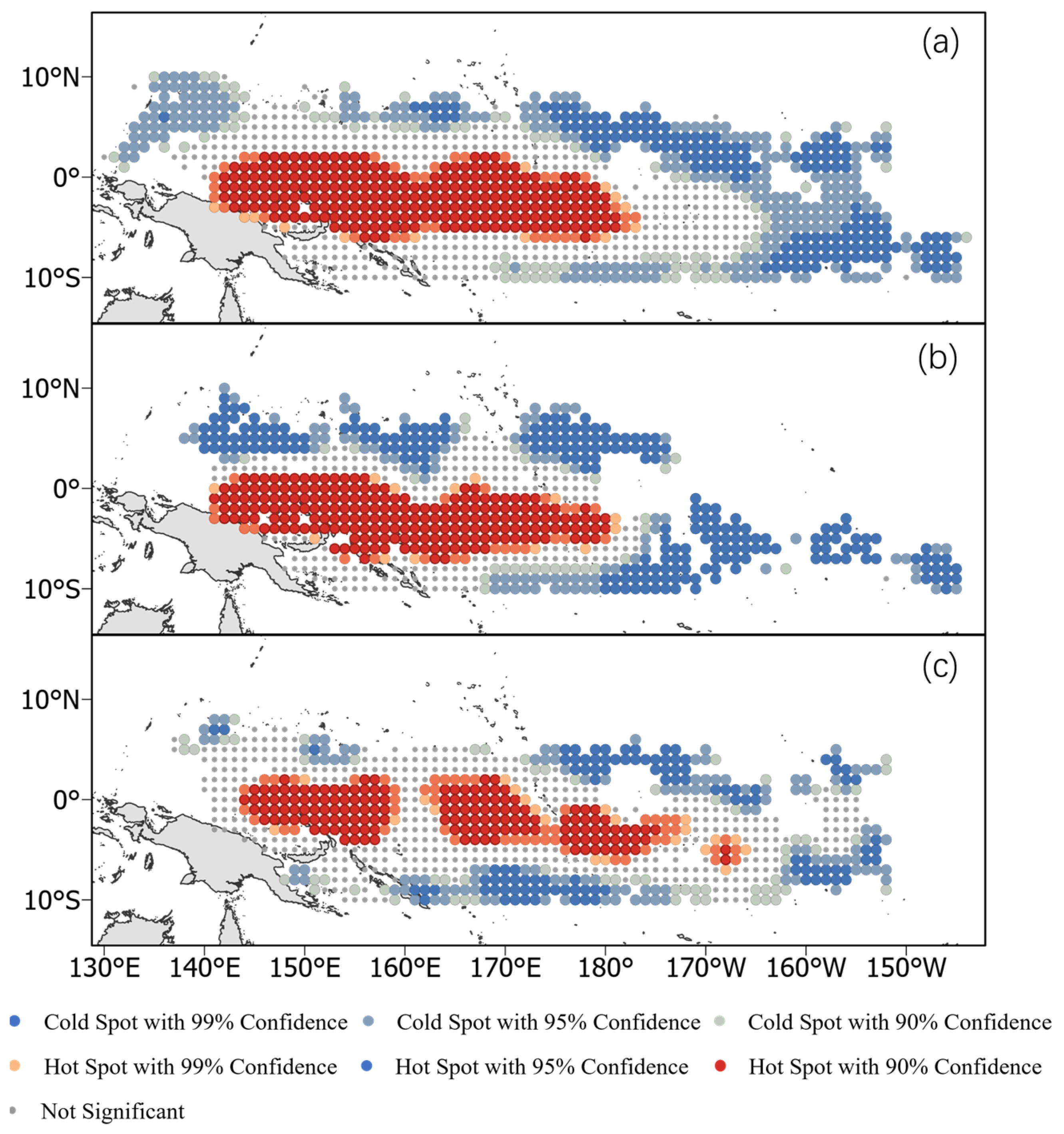
In this study, hotspot analyses were conducted on skipjack tuna catch data from 2004 to 2020, including the overall average as well as aggregated La Niña years (2008, 2011, 2016) and El Niño years (2006, 2009, 2015, 2018). The analyses aimed to identify spatial clusters of statistically significant high values (hotspots) and low values (cold spots). The features are classified into hotspots (high-value clusters), coldspots (low-value clusters), or non-significant clusters based on Gi* statistics (Figure 3).
The confidence intervals of the Gi* statistic were classified into different significance levels: 99% statistical significance, 95% statistical significance, 90% statistical significance, and no statistical significance. If a feature exhibits a high z-score and a small p-value, it indicates a spatial cluster of high values. Conversely, a low (negative) z-score with a large p-value suggests a spatial cluster of low values. The higher (or lower) the z-score, the more intense the clustering. A z-score close to zero implies no significant spatial clustering pattern.
In this study, 5% of the fishery catch data from 2021 to 2023, located in cold and hot spots with absolute Z-values greater than 2.56 and exhibiting the highest clustering density, were selected as hard data for subsequent Bayesian Maximum Entropy (BME) analysis.
It can be observed that most hotspots are concentrated in the central equatorial region, while the majority of cold spots are distributed along the peripheral areas. The spatial distribution of high catch values during the long-term historical period (2004–2020) and La Niña years is primarily concentrated in the western Pacific. In contrast, during El Niño years, the distribution of high catch values shifts significantly eastward. Notably, around the equator near 170° E, skipjack tuna catches during El Niño years are substantially higher than in surrounding areas, showing a marked difference from both the historical average and La Niña years.

3.2. Construction of Soft Data Based on the MGWR Model

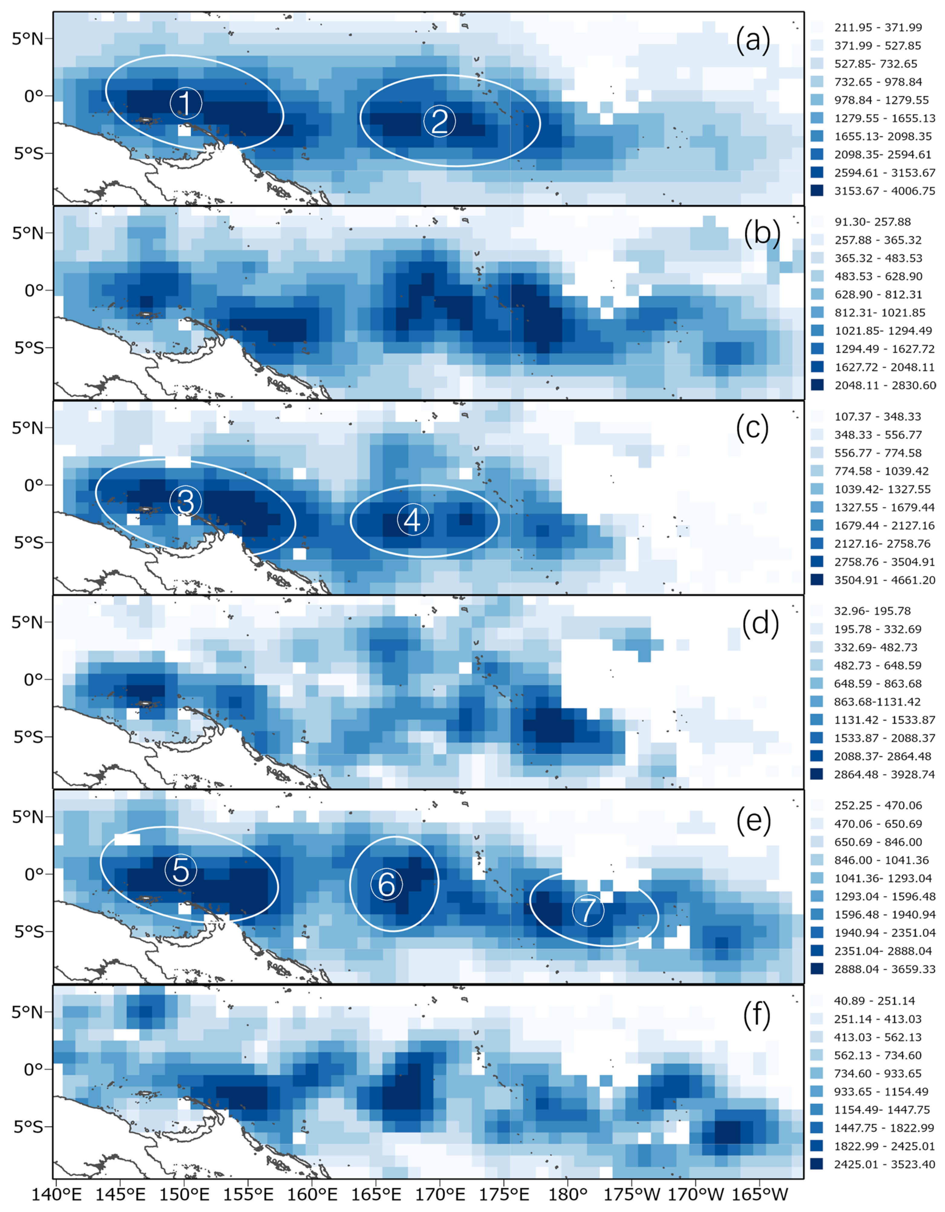
The smoothed annual average, La Niña year, and El Niño year catch data were spatially aggregated to obtain the mean and standard deviation of skipjack tuna catch within each grid cell, as shown in Figure 4.
Standard deviation is a fundamental concept in statistics, used to measure the degree of dispersion within a dataset, that is, the magnitude of variability in the data distribution [31]. In this study, the standard deviation at each grid point represents the interannual variability of skipjack tuna catch at that location, serving as the source of soft data for input into the BME model.
The spatial distributions of the annual mean catch and interannual standard deviation (std) of skipjack tuna, as shown in Figure 4, exhibit significant spatial heterogeneity, reflecting the complex spatiotemporal dynamics of skipjack tuna resources. High catch values are primarily concentrated in equatorial regions of the western Pacific, particularly in areas labeled ① through ⑥. These zones not only record high catch volumes but are also focal areas for intensive fishing activities. In contrast, low catch values are mainly observed in the eastern Pacific, where catch volumes are substantially lower than those in the western Pacific hotspots. Across the entire Pacific basin, a clear west-to-east decreasing trend in catch is evident. However, during El Niño years, certain areas in the eastern Pacific, such as region ⑦, show a slight rebound in catch, deviating from the overall declining trend.
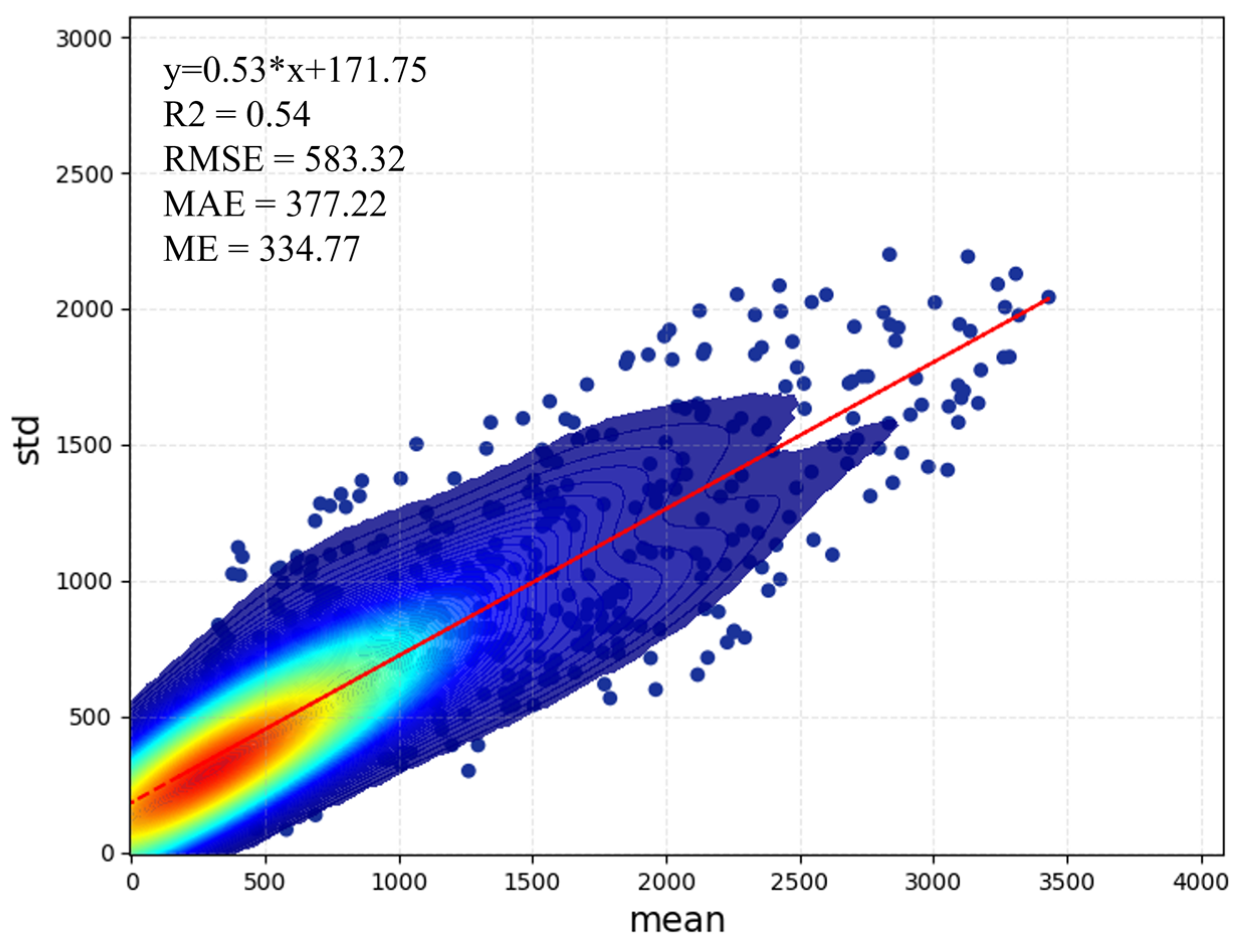
High standard deviation (std) values are primarily concentrated in regions with high catch values, while relatively stable low std values are mainly found in areas with low catch. In conjunction with Figure 3, this pattern indicates that hotspot regions are characterized by both high catch and high uncertainty, whereas cold spot regions exhibit both low catch and low uncertainty. Quantitatively, a strong correlation was observed between the mean field and the uncertainty field, with R2 of 0.54 (Figure 5).
Overall, there is a clear positive spatial correlation between the mean catch and its standard deviation (std), highlighting the high spatial heterogeneity in the distribution of skipjack tuna resources. This spatial heterogeneity underscores the importance of incorporating std as a measure of uncertainty in the BME model framework.

3.3. Comparison of Spatial Predictions from Different Models with Actual Distributions

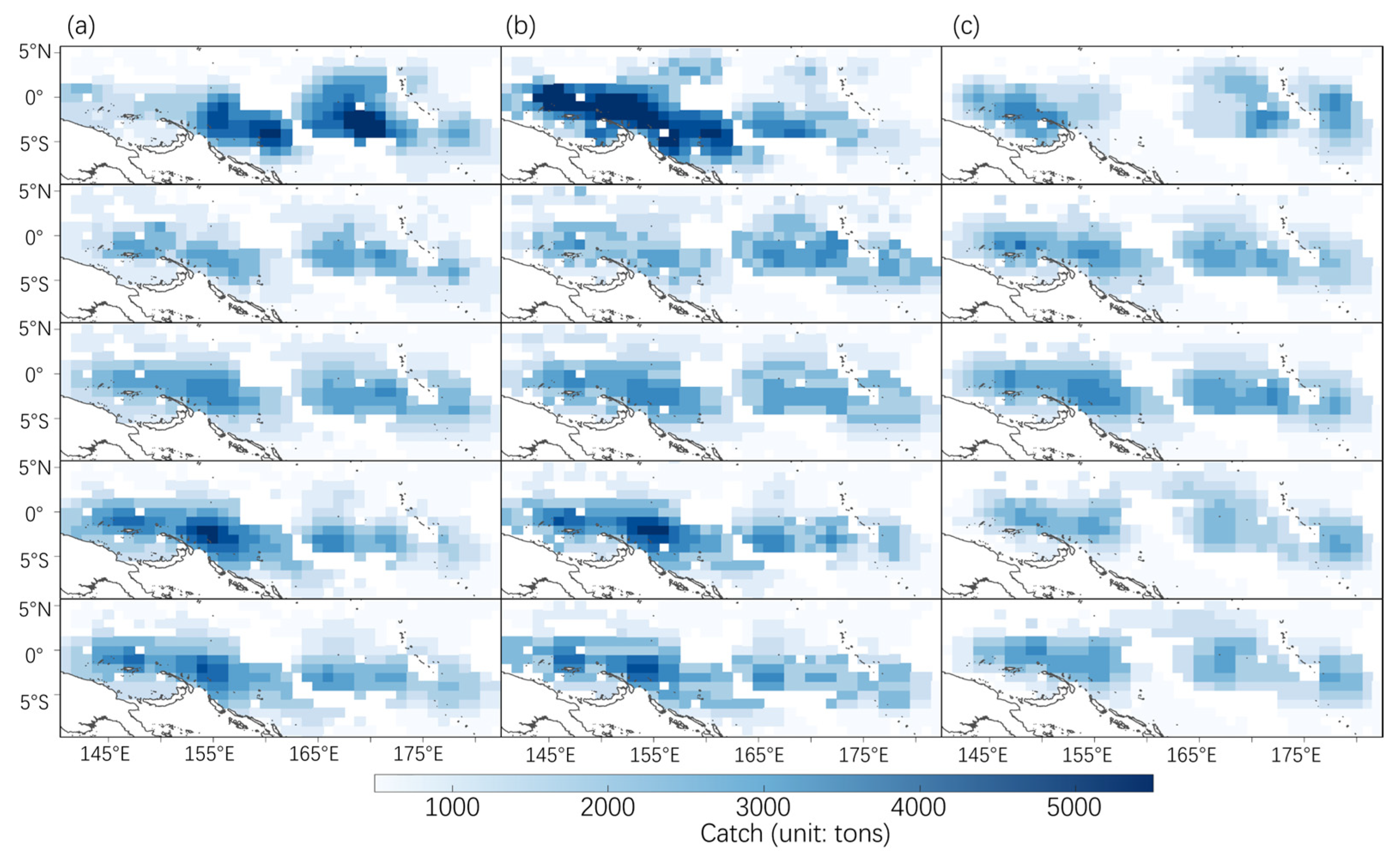
Spatial visualizations of observed versus predicted values for 2021–2023 are presented.
Figure 6 demonstrates that the catch yields in 2022 were relatively higher compared to 2021 and 2023, with high-yield areas shifting westward in the Pacific Ocean. Conversely, 2023 exhibited lower catch yields overall, with high-yield zones displaced eastward. The modeled spatial distributions of skipjack tuna catches generally aligned with observed patterns, though all models systematically underestimated high-catch regions. Notably, models incorporating ENSO types (TypeEnso) showed improved capability in capturing portions of these high-yield areas compared to other model configurations.

3.4. Model Performance Comparison

The predicted mean values are directly obtained from the MGWR model, while the prediction uncertainty is characterized by the interannual standard deviation of historical catch data. The resulting probabilistic prediction is formulated as a Gaussian distribution, N ( y ^ ,   σ ) , and used as input to the Bayesian Maximum Entropy (BME) framework to achieve an integrated prediction of skipjack tuna catch (Table 3). TypeEnso is a climate classification based on ENSO events, used to distinguish between El Niño, La Niña, and normal years. In this study, TypeEnso represents the ENSO type of different years, with 2021 and 2022 being La Niña years and 2023 being an El Niño year.
This study compared the prediction performance of different models (BME, MGWR, MGWR + TypeEnso, BME + MGWR, and BME + MGWR + TypeEnso) during 2021–2023. The R2 results showed annual variations in model performance. The BME + MGWR + TypeEnso model achieved the highest R2 values in both 2021 (0.67) and 2022 (0.62), demonstrating its strongest explanatory power during these two years. Although its R2 value decreased in 2023, it still outperformed other models.
In terms of RMSE, the BME model consistently exhibited higher values across all three years, indicating greater prediction errors. In contrast, the BME + MGWR + TypeEnso model demonstrated the lowest RMSE values in both 2021 (796.69) and 2022 (960.35), reflecting its superior prediction accuracy during these two years. For 2023, the MGWR + TypeEnso model achieved the minimum RMSE value of 784.74.
The MAE results showed similar patterns to the RMSE, with the BME model consistently yielding higher MAE values across all three years. The BME + MGWR + TypeEnso model achieved the lowest MAE values in both 2021 (557.44) and 2022 (753.39). In 2023, the BME + MGWR + TypeEnso model still maintained relatively low MAE values (591.11).
The ME values reflect the average prediction bias. Results show that all models exhibited both positive and negative ME values across the three years. Overall, the BME + MGWR + TypeEnso model demonstrated relatively smaller ME values, indicating lower prediction bias.
Integrating all evaluation metrics, the BME + MGWR + TypeEnso model demonstrated optimal overall performance in both 2021 and 2022. Although its performance slightly declined in 2023, it remained superior to other comparative models. These results indicate that the combined incorporation of BME, MGWR, and TypeEnso factors can effectively enhance the model’s predictive capability.
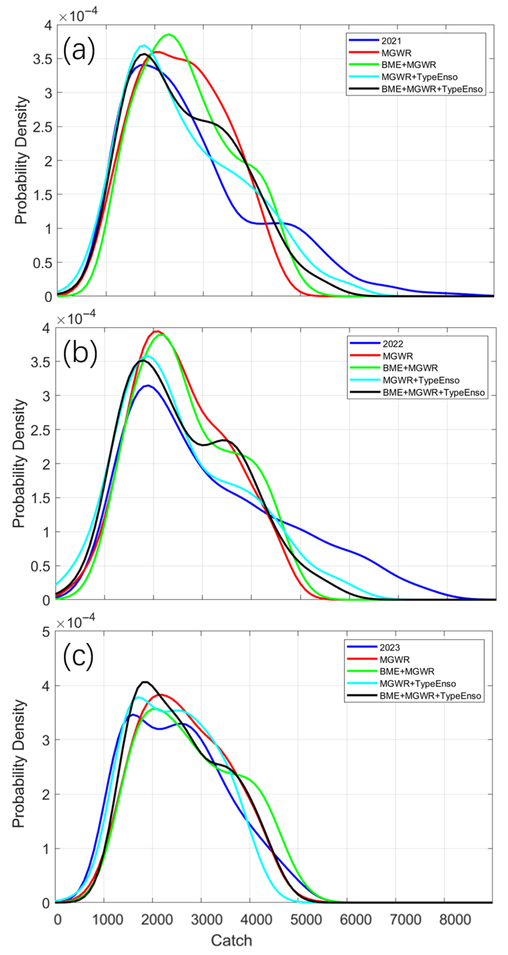
To evaluate the performance of the MGWR and MGWR-BME models in predicting skipjack tuna purse-seine catch from 2021 to 2023, this study employed Kernel Density Estimation (KDE) to visualize the distribution characteristics of both observed and predicted data. KDE is a non-parametric statistical method used to estimate the probability density function of a random variable, which clearly reveals the concentration and distribution pattern of the data [32]. The results are shown in Figure 7.
In Figure 7a, both the MGWR and MGWR-BME models, based on the historical average data from 2004 to 2020, successfully capture the main peak position. However, the MGWR prediction tends to be positively biased, with the peak slightly right-shifted, indicating an overestimation in high catch areas. The MGWR-BME model effectively corrects this bias, with its density curve more closely aligned with the observed distribution, especially showing better performance in the low-catch region. When La Niña years are used as prior knowledge, both models show improved agreement with the observed distribution, suggesting that La Niña conditions more accurately reflect the fishing environment in 2021.
Figure 7b shows that the MGWR model, based on the 2004–2020 historical average, produces a right-shifted distribution, while the MGWR-BME model corrects the tail deviation and better captures the bimodal structure seen in the observed data. Using La Niña years as prior knowledge results in both models more closely matching the observed distribution, particularly in peak location and density magnitude, further confirming the importance of distinguishing ENSO phases in prediction.
In Figure 7c, both MGWR and MGWR-BME models exhibit right-shifted peaks, with the MGWR-BME curve appearing slightly flattened, indicating underestimation of peak density. It shows limited improvement in MGWR predictions when using El Niño years as prior knowledge. However, the integrated MGWR-BME model demonstrates a clearer peak and better fit in the low-value region.
Overall, the MGWR-BME model consistently outperforms the standalone MGWR model across all years, demonstrating improved fitting accuracy. Incorporating different climate types (e.g., La Niña and El Niño) as prior knowledge can further enhance model performance, particularly during extreme climate years when environmental variability is more pronounced.

4. Discussion

4.1. Uncertainty Characterization Under Different Climatic Conditions

Combining Figure 3 and Figure 4, it can be observed that under different climatic conditions, the spatial distribution of uncertainty (standard deviation), spatial patterns (mean values), and hotspot regions exhibit significant differences. Based on the long-term historical averages from 2004 to 2020, high skipjack tuna catch values are mainly concentrated west of 180° longitude. During La Niña years, owing to the presence of warmer water environments and resource aggregation in the central and western Pacific (especially west of 180°) [33], skipjack tuna catches significantly surpass the average levels. Conversely, during El Niño years, elevated sea surface temperatures and the expansion of the warm pool in the central and western Pacific cause skipjack tuna to shift towards the edges of the warm pool, leading to an eastward displacement of fishing grounds and a decline in resource abundance [34]. This pronounced climate-driven effect not only intensifies the interannual variability of skipjack tuna distribution but also amplifies its spatial heterogeneity.
The spatial distribution characteristics of the mean catch and standard deviation (interannual variability uncertainty) of skipjack tuna in the central and western Pacific indicate significant spatial aggregation and interannual variability of the resource (Figure 4). High catch zones are primarily located in the core area of the warm pool west of 180°, where the sea surface temperature consistently ranges between 28 °C and 30 °C throughout the year [35], providing an optimal habitat for skipjack tuna. Notably, these high-yield regions spatially coincide with areas of elevated catch standard deviation, suggesting a strong correlation (R2 = 0.54) between resource abundance and interannual variability [36]. Ocean currents and upwelling near the equatorial region play a crucial role in shaping the distribution of skipjack tuna. Upwelling brings abundant prey organisms, which facilitate the reproduction and growth of skipjack tuna. However, these oceanographic processes exhibit significant variability in the equatorial region, resulting in pronounced interannual fluctuations of skipjack tuna resources [37,38]. In contrast, sea surface temperature and salinity north of the equator tend to be more stable, lacking the pronounced seasonal and interannual variability observed near the equator [39]. The equatorial Pacific region exhibits particularly prominent interannual variability features, characterized by clusters of high standard deviation values, underscoring the critical regulatory role of climate variability on fishery resource distribution [40]. Key environmental parameters in this region, such as chlorophyll concentration and thermocline depth, show high sensitivity to the Niño 3.4 index. This close coupling directly influences interannual fluctuations in catch by altering skipjack tuna aggregation behavior.
In regions with favorable environmental conditions, skipjack tuna resources tend to aggregate densely, resulting in pronounced catch peaks within specific areas. Concurrently, influenced by the interannual variability of environmental factors, these regions exhibit substantial spatiotemporal fluctuations in resource abundance, leading to zones of high standard deviation. It is noteworthy that the spatial distribution of environmental factors in the central and western Pacific itself displays significant heterogeneity [41]. This uneven distribution drives skipjack tuna to concentrate in certain habitats. Moreover, the interannual variability of environmental factors further amplifies the fluctuations in resource distribution, ultimately causing a spatial overlap between high-catch zones and areas of elevated standard deviation.
Based on these findings, this study developed catch distribution models under varying climatic conditions, providing new evidence for understanding the regulatory role of mesoscale oceanic processes on fishery resources. Notably, the pronounced uncertainty characteristics in the equatorial Pacific region highlight its critical role as a key component in the climate–fishery coupled system.

4.2. Analysis of Spatial Variability in Skipjack Tuna Catch Under Different Climate Types

This study found that models constructed based on different climate types can significantly improve predictive performance. During the early phase of the 2021 La Niña event, due to minimal variations in environmental factors, predictions based on historical La Niña data did not show a marked advantage. However, by 2022, the model’s R2 increased by approximately 50%. This discrepancy in predictive accuracy primarily arises from the differentiated impacts of ENSO events on the marine environment. During La Niña events, enhanced upwelling of cold water in the eastern Pacific leads to increased nutrient input and significantly improves primary productivity, an environmental shift characterized by high interannual repeatability [42]. The MGWR model, through geographically weighted regression, effectively captures this spatial consistency, with its local linear properties well reflecting the relatively stable environment–fishery relationships during La Niña periods.
However, El Niño events exhibit more complex oceanic response mechanisms, including pronounced typological differences between the Eastern Pacific (EP) and Central Pacific (CP) variants [11,43]. These differences not only affect sea surface temperature distributions but also significantly alter upwelling intensity, nutrient availability, and primary productivity patterns, leading to a marked increase in spatial heterogeneity of the marine environment. Notably, the strong El Niño event in 2023 caused an anomalous eastward expansion of the Western Pacific Warm Pool, substantially disrupting the traditional distribution patterns of skipjack tuna. Consequently, predictions based on historical El Niño year data still exhibited considerable deviations.
Based on the kernel density estimation (KDE) curves in Figure 6, the distribution characteristics of observed and predicted values were visualized. The models demonstrated better fitting performance in low-value regions of skipjack tuna in the central-west Pacific, while their fit was comparatively poorer in high-value regions. The results indicate that modeling based solely on historical data struggles to fully capture the complex climate-environment interactions. Although the MGWR model incorporates some environmental factors, its representation remains limited and cannot completely reveal the impact of environmental changes on catch variability. Additionally, some potential influencing factors and interactions among environmental variables are not considered in the model. In this context, introducing a composite categorical factor—climate type, which can significantly improve the model’s predictive performance.

4.3. Application of the Integrated MGWR-BME Method in Skipjack Tuna Prediction

The distribution of fishery resources exhibits a complex pattern characterized by mean field features superimposed with random fluctuations. Its high mobility and spatiotemporal variability pose significant challenges for accurate modeling [44]. The BME method focuses on quantifying uncertainty in fishery resource assessment. Its dynamic data fusion mechanism, based on Bayesian inference and the probability distribution selection guided by the maximum entropy principle [45], enables the model to adapt to the non-normality and spatiotemporal variability inherent in fishery data. However, for fisheries as a dynamic resource, using the mean catch directly in the BME model is inappropriate. Therefore, this study employs the MGWR model to characterize the mean state of resource distribution. By incorporating geographically weighted parameters, MGWR effectively captures the spatial heterogeneity of environmental influences, accurately reflecting regional differences in the environment–catch relationships across different marine areas. Compared with traditional global regression models such as GWR and GAM, MGWR more flexibly represents the spatial variations in environment–catch relationships, providing higher-precision [46] soft data support.
MGWR demonstrates three key advantages: First, its multiscale modeling capability enables accurate identification of characteristic operational scales for different driving variables, effectively preventing local adaptability deficiencies or overfitting issues caused by uniform bandwidth. Second, by generating spatially explicit varying coefficient surfaces, it quantitatively reveals spatial differentiation patterns in environmental factor influence intensity, providing scientific support for precision fisheries management. Third, the model’s adaptive smoothing mechanism automatically adjusts local weighting ranges according to variable spatial heterogeneity levels, ensuring more robust regression results.
Traditional BME models are based on a deterministic framework, which limits their applicability in studying highly dynamic marine resources. In contrast, integrating MGWR with BME effectively overcomes the challenges faced by conventional BME methods in this field. The spatial regression results generated by MGWR provide a reliable source of soft data for BME, while the maximum entropy optimization process of BME further enhances the robustness of model predictions [47]. The study found that when predicting based on different climate types, the BME model improved the MGWR model’s performance by 14% in 2021, 2% in 2022, and 8% in 2023. This synergistic effect was well demonstrated in skipjack tuna predictions, where the model not only accurately identified high-yield areas near the equatorial upwelling zones but also reasonably captured the gradient features of low-yield offshore regions.
The integration of MGWR and BME leverages the complementary strengths of both methods, establishing a more robust and flexible spatial data analysis framework. This study is the first to develop an integrated BME-MGWR model based on prior knowledge and environmental variables, which effectively predicts the distribution of skipjack tuna resources in the central and western Pacific.
However, the current approach still has certain limitations. The limited observations of environmental factors and the complexity of their interactions constrain the model’s ability to fully capture the dynamic changes in the resources. In particular, climate types are a composite of multiple environmental factors, and their influence mechanisms remain to be thoroughly elucidated [48]. Meanwhile, the highly mobile nature of fishery resources makes it difficult to apply traditional time series analysis methods directly. To reduce the risk of data noise, this study employs temporal averaging, which, while improving model stability, inevitably sacrifices some temporal dynamic information.

5. Conclusions

This study proposes an improved spatial prediction framework (BME-MGWR) to enhance the forecasting capability of skipjack tuna (Katsuwonus pelamis) resource distribution in the western and central Pacific Ocean under complex climatic conditions. The results reveal a significant correlation between skipjack catch and standard deviation, which provides scientific evidence for understanding the spatial heterogeneity of fishery resources. The framework employs the MGWR model to capture the multiscale variation characteristics of environmental factors while integrating prior knowledge and spatial uncertainty through the BME model. Compared with single-model approaches, the proposed framework demonstrates superior prediction accuracy and applicability, particularly in distinguishing different climate regimes. While fishermen’s empirical knowledge can identify historically productive fishing grounds, our model provides pre-adaptive capacity under climate variability by elucidating the relationship between ENSO and resource distribution patterns. Then, the model still exhibits considerable prediction bias in high-catch areas, which may be attributed to the complexity of environmental or biological interactions. The BME-MGWR framework effectively integrates multiscale environmental variability and spatial uncertainty, providing novel methodological support for predicting fishery dynamics under climate change. The accurate prediction of high-catch and low-catch areas in this study can provide a scientific decision-making basis for fishery managers, effectively reducing unnecessary consumption of human and material resources. It offers flexible ideas for addressing the risk of species endangerment, thereby laying a solid foundation for the sustainable development of fisheries. Nevertheless, the exclusion of dynamic anthropogenic factors such as fishing pressure may limit the model’s long-term prediction accuracy. Future research could incorporate machine learning or deep learning techniques to improve high-catch area predictions while accounting for human activities. Overall, this study offers an important scientific basis and practical guidance for sustainable fisheries management under climate change, demonstrating significant theoretical value and application potential.

Author Contributions

Conceptualization, Y.W. and X.Y.; methodology, Y.W.; software, M.L.; validation, M.L.; formal analysis, X.Y.; investigation, Y.W.; resources, X.Y.; data curation, M.L.; writing—original draft preparation, Y.W.; writing—review and editing, J.Z.; visualization, Y.W.; supervision, X.Y.; project administration, X.Y.; funding acquisition, J.Z. All authors have read and agreed to the published version of the manuscript.

Funding

This research was funded by the National Key R&D Programs of China (2024YFD2400603).

Institutional Review Board Statement

Not applicable.

Informed Consent Statement

Informed consent was obtained from all subjects involved in the study.

Data Availability Statement

The data presented in this study are openly available in WCPFC’s official database/reporting system at https://www.wcpfc.int/ (accessed on 10 November 2024).

Acknowledgments

This project was funded in part by the National Key Research and Development Program of China. We thank all our colleagues from the Research Laboratory for their work in data collection.

Conflicts of Interest

The authors declare no conflicts of interest.

References

  1. Collette, B.N. FAO Species Catalogue; FAO: Rome, Italy, 1983; Volume 2, Scombrids of the world. An annotated and illustrated catalogue of tunas, mackerels, bonitos and related species known to date.
  2. Sarkka, S.; Hartikainen, J. On Gaussian optimal smoothing of non-linear state space models. IEEE Trans. Autom. Control 2010, 18, 1938–1941. [Google Scholar] [CrossRef]
  3. Hilborn, R. Modeling the Stability of Fish Schools: Exchange of Individual Fish between Schools of Skipjack Tuna (Katsuwonus pelamis). Can. J. Fish. Aquat. Sci. 1991, 48, 1081–1091. [Google Scholar] [CrossRef]
  4. Lehodey, P.; Bertignac, M.; Hampton, J.; Lewis, A.; Picaut, J. El Nino Southern Oscillation and tuna in the western Pacific. Nature 1997, 389, 715–718. [Google Scholar] [CrossRef]
  5. Picaut, J.; Ioualalen, M.; Menkes, C.; Delcroix, T.; McPhaden, M.J. Mechanism of the zonal displacements of the Pacific warm pool: Implications for ENSO. Science 1996, 274, 1486–1489. [Google Scholar] [CrossRef]
  6. Mugo, R.; Saitoh, S.-I.; Nihira, A.; Kuroyama, T. Habitat characteristics of skipjack tuna (Katsuwonus pelamis) in the western North Pacific: A remote sensing perspective. Fish. Oceanogr. 2010, 19, 382–396. [Google Scholar] [CrossRef]
  7. Wang, Y.; Yang, X.M.; Zhu, J.F. Oscillation mode analysis on time series of the abundance of unassociated school Katsuwonus pelamis in the Western and Central Pacific Ocean. Mar. Fish. 2024, 46, 266–274. (In Chinese) [Google Scholar] [CrossRef]
  8. Alfatinah, A.; Chu, H.-J.; Tatas, S.R.; Patra, S.R. Fishing Area Prediction Using Scene-Based Ensemble Models. J. Mar. Sci. Eng. 2023, 11, 1398. [Google Scholar] [CrossRef]
  9. Puspita, A.R.; Syamsuddin, M.L.; Subiyanto; Syamsudin, F.; Purba, P.N. Predictive Modeling of Eastern Little Tuna (Euthynnus affinis) Catches in the Makassar Strait Using the Generalized Additive Model. J. Mar. Sci. Eng. 2023, 11, 165. [Google Scholar] [CrossRef]
  10. Hidayat, R.; Zainuddin, M.; Mallawa, A.; Mustapha, M.A.; Putri, A.R.S. Estimating potential fishing zones for Skipjack Tuna (Katsuwonus pelamis) Abundance in Southern Makassar Strait. IOP Conf. Ser. Earth Environ. Sci. 2020, 564, 012082. [Google Scholar] [CrossRef]
  11. Yen, K.-W.; Wang, G.; Lu, H.-J. Evaluating habitat suitability and relative abundance of skipjack (Katsuwonus pelamis) in the Western and Central Pacific during various El Nino events. Ocean Coast. Manag. 2017, 139, 153–160. [Google Scholar] [CrossRef]
  12. Silva, C.; Leiva, F.; Lastra, J. Predicting the current and future suitable habitat distributions of the anchovy (Engraulis ringens) using the Maxent model in the coastal areas off central-northern Chile. Fish. Oceanogr. 2019, 28, 171–182. [Google Scholar] [CrossRef]
  13. Wang, W. Quantifying the spatial nonstationary response of environmental factors on purse seine tuna vessel fishing. Heliyon 2024, 10, e33298. [Google Scholar] [CrossRef]
  14. Liu, L. An integrative machine learning approach to understanding South Pacific Ocean albacore tuna habitat features. ICES J. Mar. Sci. 2025, 82, fsaf003. [Google Scholar] [CrossRef]
  15. Zhu, H. Improving XCO2 retrieval under high aerosol loads with fused satellite aerosol Data: Advancing understanding of anthropogenic emissions. ISPRS J. Photogramm. Remote Sens. 2025, 223, 146–158. [Google Scholar] [CrossRef]
  16. He, J.; Christakos, G.; Wu, J.; Li, M.; Leng, J. Spatiotemporal BME characterization and mapping of sea surface chlorophyll in Chesapeake Bay (USA) using auxiliary sea surface temperature data. Sci. Total Environ. 2021, 794, 148670. [Google Scholar] [CrossRef]
  17. Zhang, C.; Yang, Y. Can the spatial prediction of soil organic matter be improved by incorporating multiple regression confidence intervals as soft data into BME method? CATENA 2019, 178, 322–334. [Google Scholar] [CrossRef]
  18. Wang, F.; Liu, X.; Bergquist, R.; Lv, X.; Liu, Y.; Gao, F.; Li, C.; Zhang, Z. Bayesian maximum entropy-based prediction of the spatiotemporal risk of schistosomiasis in Anhui Province, China. BMC Infect. Dis. 2021, 21, 1171. [Google Scholar] [CrossRef]
  19. Ghazipour, F.; Mahjouri, N. A multi-model data fusion methodology for seasonal drought forecasting under uncertainty: Application of Bayesian maximum entropy. J. Environ. Manag. 2022, 304, 114245. [Google Scholar] [CrossRef]
  20. Arrizabalaga, H.; Dufour, F.; Kell, L. Global habitat preferences of commercially valuable tuna. Elsevier 2015, 113, 102–112. [Google Scholar] [CrossRef]
  21. Langley, A.; Hampton, J.; Ogura, M. Stock assessment of skipjack tuna in the western and central Pacific Ocean. In Proceedings of the First Meeting of the Scientific Committee of the Western and Central Pacific Fisheries Commission, Working Paper, New Caledonia, France, 8–19 August 2005; Volume 4, p. 68. [Google Scholar]
  22. Anderson, G.; Lal, M.; Stockwell, B.; Hampton, J.; Smith, N.; Nicol, S.; Rico, C. No Population Genetic Structure of Skipjack Tuna (Katsuwonus pelamis) in the Tropical Western and Central Pacific Assessed Using Single Nucleotide Polymorphisms. Front. Mar. Sci. 2022, 7, 570760. [Google Scholar] [CrossRef]
  23. Wang, P.; Deng, H.; Wang, Y.M.; Liu, Y.; Zhang, Y. Kernel Density Estimation Based Gaussian and Non-Gaussian Random Vibration Data Induction for High-Speed Train Equipment. IEEE Access 2020, 8, 90914–90923. [Google Scholar] [CrossRef]
  24. Souris, M.; Demoraes, F. Improvement of Spatial Autocorrelation, Kernel Estimation, and Modeling Methods by Spatial Standardization on Distance. ISPRS Int. J. Geo Inf. 2019, 8, 199. [Google Scholar] [CrossRef]
  25. Singh, P.P.; Sabnani, C.S.; Kapse, V.S. Hotspot Analysis of Structure Fires in Urban Agglomeration: A Case of Nagpur City, India. Fire 2021, 4, 38. [Google Scholar] [CrossRef]
  26. Xinming, Z.; Xiaoning, S.; Pei, L.; Ronghai, H.U. Spatial downscaling of land surface temperature with the multi-scale geographically weighted regression. Natl. Remote Sens. Bull. 2021, 25, 1749–1766. [Google Scholar] [CrossRef]
  27. Christakos, G. Spatiotemporal information systems in soil and environmental sciences. Geoderma 1998, 85, 141–179. [Google Scholar] [CrossRef]
  28. Zhang, C.T. Research on Key Issues and Applications of Spatiotemporal Prediction Using Bayesian Maximum Entropy Method. Ph.D. Thesis, Huazhong Agricultural University, Wuhan, China, 2017. (In Chinese). [Google Scholar]
  29. Farooq, N.; Patterson, A.J.; Walsh, S.R.; Prytherch, D.R.; Justin, T.A.; Tang, T.Y. R2: A useful measure of model performance when predicting a dichotomous outcome. Stat. Med. 1999, 18, 375–384. [Google Scholar] [CrossRef]
  30. Moraes, C.P.A.; Fantinato, D.G.; Neves, A. Epanechnikov kernel for PDF estimation applied to equalization and blind source separation. Signal Process. 2021, 189, 108251. [Google Scholar] [CrossRef]
  31. Streiner, D.L. Maintaining standards: Differences between the standard deviation and standard error, and when to use each. Can. J. Psychiatry 1996, 41, 498–502. [Google Scholar] [CrossRef] [PubMed]
  32. Dai, J.; Liu, Y.; Chen, J.; Liu, X. Fast feature selection for interval-valued data through kernel density estimation entropy. Int. J. Mach. Learn. Cybern. 2020, 11, 2607–2624. [Google Scholar] [CrossRef]
  33. Hartoko, A.; Suradi, W.S.; Ghofar, A. Impact of climate variability on skipjack tuna (Katsuwonus pelamis) catches in the Indonesian Fisheries Management Area (FMA) 715. In IOP Conference Series: Earth and Environmental Science; IOP Publishing: London, UK, 2021; Volume 800, p. 012003. [Google Scholar] [CrossRef]
  34. Hartoko, A.; Saputra, S.W.; Ghofar, A.; Nugraha, E. Impact of El Niño Southern Oscillation (ENSO), variability on skipjack tuna (Katsuwonus pelamis) catches in the fisheries management area (FMA) 715, Indonesia. AACL Bioflux 2021, 14, 1685–1694. [Google Scholar]
  35. Hu, K.W.; Zhu, G.P.; Wang, X.F.; Xu, L.X. Spatio-temporal distribution of skipjack tuna(Katsuwonus pelamis) abundance and its relationship with sea surface temperature in Western and Central Pacific Ocean. Mar. Fish. 2022, 33, 417–422. (In Chinese) [Google Scholar] [CrossRef]
  36. Druon, J.-N.; Chassot, E.; Murua, H.; Lopez, J. Skipjack Tuna Availability for Purse Seine Fisheries Is Driven by Suitable Feeding Habitat Dynamics in the Atlantic and Indian Oceans. Front. Mar. Sci. 2017, 4, 315. [Google Scholar] [CrossRef]
  37. Chen, Y.Y.; Chen, X.J.; Guo, L.X.; Fang, Z. Fishing ground forecasting on Katsuwonus pelamis based on different climatic conditions in western and central Pacific Ocean. J. Shanghai Ocean. Univ. 2019, 28, 145–153. (In Chinese) [Google Scholar]
  38. Wang, J.T.; Chen, X.J. Changes and Prediction of the Fishing Ground Gravity of Skipjack (Katsuwonus pelamis) in Western-Central Pacific. Period. Ocean. Univ. China 2013, 43, 44–48. (In Chinese) [Google Scholar]
  39. Ma, Y.C. Influence of environmental factors on CPUE of three different fishing methods in skipjack tuna fisheries. South China Fish. Sci. 2023, 19, 11–20. (In Chinese) [Google Scholar]
  40. Lehodey, P. Climate variability, fish, and fisheries. J. Clim. 2006, 19, 5009–5030. [Google Scholar] [CrossRef]
  41. Tseng, C.-T.; Sun, C.-L.; Yeh, S.-Z.; Chen, S.-C.; Su, W.-C. Spatio-temporal distributions of tuna species and potential habitats in the Western and Central Pacific Ocean derived from multi-satellite data. Int. J. Remote Sens. 2010, 31, 4543–4558. [Google Scholar] [CrossRef]
  42. Geng, T.; Jia, F.; Cai, W.; Wu, L.; Gan, B.; Jing, Z.; Li, S.; McPhaden, M.J. Increased occurrences of consecutive La Nina events under global warming. Nature 2023, 619, 774–781. [Google Scholar] [CrossRef] [PubMed]
  43. Liu, Y.; Donat, M.G.; England, M.H.; Alexander, L.V.; Hirsch, A.L.; Delgado-Torres, C. Enhanced multi-year predictability after El Nino and La Nina events. Nat. Commun. 2023, 14, 6387. [Google Scholar] [CrossRef] [PubMed]
  44. Kim, J.; Na, H.; Park, Y.-G.; Kim, Y.H. Potential predictability of skipjack tuna (Katsuwonus pelamis) catches in the Western Central Pacific. Sci. Rep. 2020, 10, 3193. [Google Scholar] [CrossRef]
  45. D’Or, D.; Bogaert, P. Spatial prediction of categorical variables with the Bayesian Maximum Entropy approach: The Ooypolder case study. Eur. J. Soil Sci. 2004, 55, 763–775. [Google Scholar] [CrossRef]
  46. Zheng, H.H.; Yang, X.M.; Zhu, J.F. Environmental impact mechanism of skipjack tuna fishery in Western and Central Pacific Ocean based on Multi-scale Geographical Weighted Regression Model (MGWR). South China Fish. Sci. 2023, 19, 1–10. (In Chinese) [Google Scholar]
  47. Hanigan, I.C.; Yu, W.; Yuen, C.; Gopi, K.; Knibbs, L.D.; Cowie, C.T.; Jalaludin, B.; Cope, H.M.; Riley, M.L. Heyworth Deep ensemble machine learning with Bayesian blending improved accuracy and precision of modelled ground-level ozone for region with sparse monitoring: Australia, 2005–2018. Environ. Model. Softw. 2025, 187, 106378. [Google Scholar] [CrossRef]
  48. Liu, Z.; Li, J.; Zhang, J.; Chen, Z.; Zhang, K. Climate Variability and Fish Community Dynamics: Impacts of La Niña Events on the Continental Shelf of the Northern South China Sea. J. Mar. Sci. Eng. 2025, 13, 474. [Google Scholar] [CrossRef]
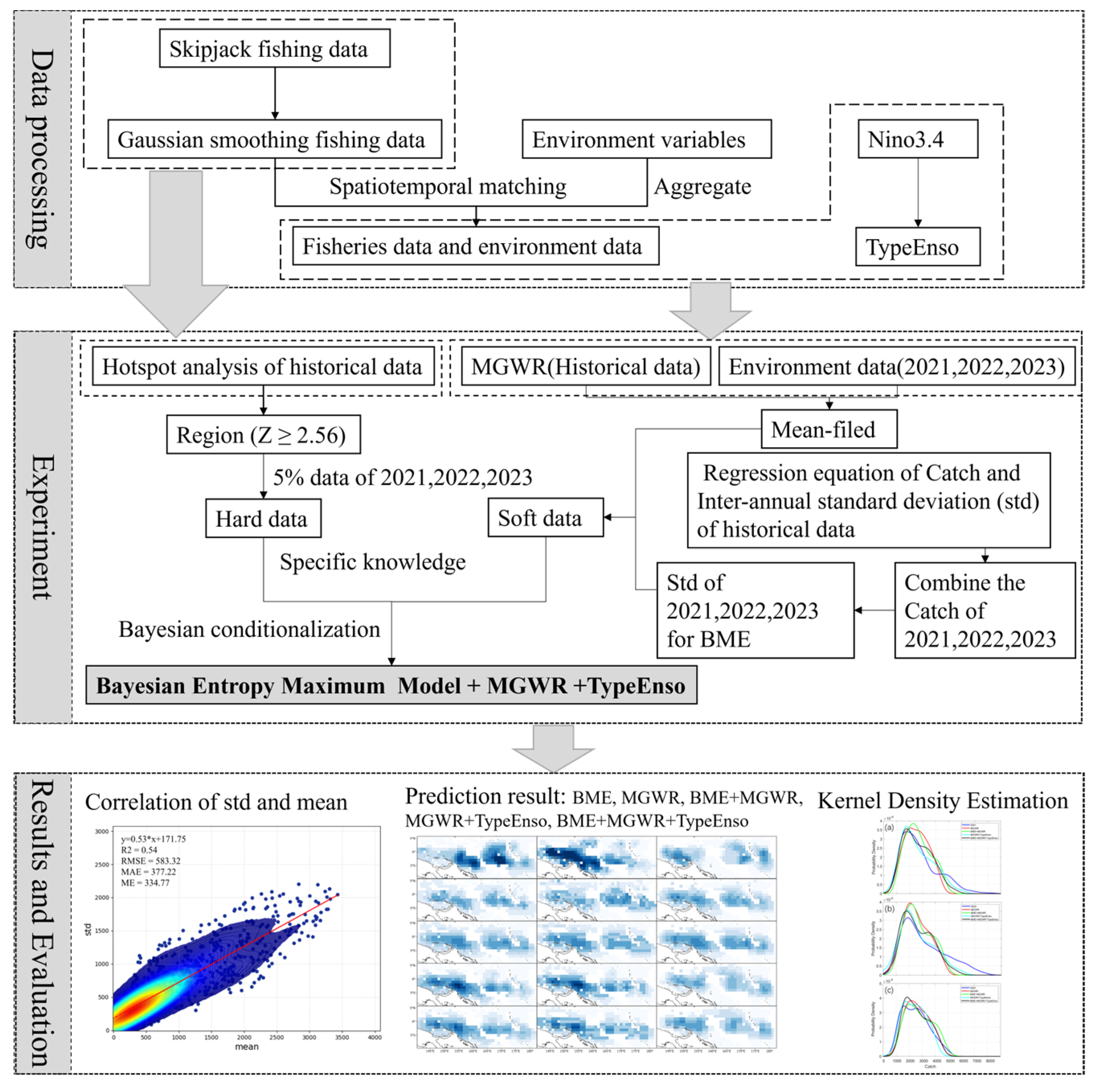
Figure 1. An illustration of the workflow implemented in this study.
Fishes 10 00450 g001
Figure 2. The warm pool-cold tongue ecosystem in the Western and Central Pacific Ocean (the red box indicates the study area).
Fishes 10 00450 g002
Figure 3. Hotspot analysis of annual mean skipjack tuna catch in the Western and Central Pacific Ocean: (a) 2004–2020 overall average; (b) aggregated La Niña years; (c) aggregated El Niño years.
Fishes 10 00450 g003
Figure 4. Spatial distribution of aggregated purse seine skipjack tuna catch in the Western and Central Pacific Ocean (Unit: tons): (a) annual mean Catch (2004–2020); (b) standard deviation of annual catch (2004–2020); (c) annual mean catch during La Niña years; (d) standard deviation of annual catch during La Niña years; (e) annual mean catch during El Niño years; (f) standard deviation of annual catch during El Niño years.
Fishes 10 00450 g004
Figure 5. The correlation of std and the mean.
Fishes 10 00450 g005
Figure 6. Spatial distribution maps of skipjack tuna catch in the Western and Central Pacific Ocean. (a) 2021; (b) 2022; (c) 2023. (Row 1: Smoothed spatial distribution for 2021–2023; Row 2: MGWR results; Row 3: BME + MGWR results; Row 4: MGWR+TypeEnso results; Row 5: BME + MGWR + TypeEnso results).
Fishes 10 00450 g006
Figure 7. Kernel density estimation (KDE) characteristic curves of observed versus predicted purse seine skipjack tuna catches for 2021–2023: (a) 2021; (b) 2022; (c) 2023.
Fishes 10 00450 g007
Table 1. Environmental variables and data sources.
VariableUnitSource
SLAmhttp://marine.copernicus.eu/ accessed on 1 March 2023
MLDmhttp://www.science.oregonstate.edu/
CHLMg/m2/day
T5, T55, T105°Chttp://www.argo.org.cn/
SSSPSS-78
V55, U55m/shttps://cfs.ncep.noaa.gov/
Table 2. Variance inflation factors (VIF) of environmental variables.
VariableVIF
SLA1.12
MLD4.00
CHL1.70
SSS4.01
T56.97
T555.18
T1053.65
V551.24
U551.37
Table 3. Predicted results of MGWR and MGWR-BME models for the years 2021–2023.
ModelR2RMSEMAEME
2021BME0.091627.461104.43983.29
MGWR0.53946.83687.49240.95
MGWR + TypeEnso0.441037.98786.54157.48
BME + MGWR0.60870.75577.61300.51
BME + MGWR + TypeEnso0.67796.69557.44216.84
2022BME0.061895.521319.41256.32
MGWR0.231404.941070.65534.37
MGWR + TypeEnso0.61988.82753.82552.3
BME + MGWR0.341297.51857.42717.34
BME + MGWR + TypeEnso0.62960.35753.39525.07
2023BME0.031169.36874.85686.49
MGWR0.26835.46667.97−126.97
MGWR + TypeEnso0.37784.74616.9892.81
BME + MGWR0.30804.77622.56124.11
BME + MGWR + TypeEnso0.40777.99591.11146.21
Disclaimer/Publisher’s Note: The statements, opinions and data contained in all publications are solely those of the individual author(s) and contributor(s) and not of MDPI and/or the editor(s). MDPI and/or the editor(s) disclaim responsibility for any injury to people or property resulting from any ideas, methods, instructions or products referred to in the content.