Article

Spatial Heterogeneity-Based Explainable Machine Learning Methods—Modeling the Relationship Between Yellowfin Tuna Fishery Resources and the Environment in the Pacific Ocean

1
College of Marine Living Resource Sciences and Management, Shanghai Ocean University, Shanghai 201306, China
2
National Engineering Research Center for Oceanic Fisheries, Shanghai Ocean University, Shanghai 201306, China
3
Key Laboratory of Sustainable Exploitation of Oceanic Fisheries Resources, Ministry of Education, Shanghai 201306, China
4
Key Laboratory of Oceanic Fisheries Exploration, Ministry of Agriculture and Rural Affairs, Shanghai 201306, China
5
Scientific Observing and Experimental Station of Oceanic Fishery Resources, Ministry of Agriculture and Rural Affairs, Shanghai 201306, China
*
Author to whom correspondence should be addressed.
Fishes 2025, 10(8), 417; https://doi.org/10.3390/fishes10080417
Submission received: 7 July 2025 / Revised: 8 August 2025 / Accepted: 16 August 2025 / Published: 19 August 2025
(This article belongs to the Section Environment and Climate Change)

Abstract

Yellowfin tuna (Thunnus albacares) constitutes a critical global fishery resource, and its distribution pattern is correlated to varying degrees with the marine environment. This study utilized longline fishing data from the Western and Central Pacific Fisheries Commission (WCPFC) and the Inter-American Tropical Tuna Commission (IATTC) spanning 2004 to 2020, categorized by quarter and combined with surface and 0–200 m depth environmental variables. Geographical random forests (GRF) were employed to examine spatially non-stationary relationships between yellowfin tuna resources and environmental factors. Additionally, by integrating GRF with GeoShapley explainable methods, we quantitatively evaluated the mechanistic impacts of environmental drivers on tuna distribution across spatial scales. The findings indicated that (1) the GRF model demonstrated superior performance throughout all four quarters, with the goodness of fit on the 20% test set (R2 = 0.72–0.85) consistently surpassing that of conventional random forest (RF) (R2 = 0.68–0.79) and extreme gradient boosting random forest (XGBRF) (R2 = 0.68–0.80). Moreover, in most cases, it had a lower RMSE and MAE, while effectively addressing spatial heterogeneity issues in yellowfin tuna fishery resources across most regions. (2) GeoShapley spatial explainable analysis revealed distinct environmental drivers, showing that the sea surface temperature and temperature at 105 m depth significantly influenced yellowfin tuna resources across all quarters, following a “high-value promotion, low-value inhibition” pattern, with salinity and dissolved oxygen at 105 m depth in Q2–Q3 and mixed-layer depth in Q3 also demonstrating notable effects. (3) Significant spatiotemporal heterogeneity was observed. The main spatial effects and temperature–depth–locality interactions remained significant throughout the year; mixed-layer depth–locality interactions were prominent in Q1, Q3, and Q4, dissolved oxygen–locality interactions in Q2 and Q4, and 105 m salinity–locality interactions exclusively in Q2. This study used geographical random forests (GRF) to integrate spatial statistics and machine learning to model the relationship between Pacific yellowfin tuna fishery resources and environmental factors. This approach demonstrates potential in improving spatial predictions of heterogeneous tuna resources and may help to identify key environmental drivers influencing their distribution. These findings provide essential insights for the formulation of science-based management strategies for Pacific yellowfin tuna fisheries.
Key Contribution: Compared with traditional machine learning and explainable methods used in the field of fishery resources, this study introduces machine learning methods that consider spatial heterogeneity and explainable methods based on spatial effects, providing new insights for fishery resource management.

1. Introduction

The yellowfin tuna (Thunnus albacares) is a highly migratory species [1], primarily inhabiting pelagic waters of tropical and subtropical zones worldwide [2]. As a dominant target species in longline fisheries [3], its Pacific catch contributes substantially to global yields [4], occupying a pivotal position in tuna fisheries. The Pacific Ocean exhibits complex spatial heterogeneity, presenting unique challenges for the modeling of yellowfin tuna fishery resources. Spanning over 15,000 km from east to west, the region encompasses diverse marine environmental systems, including the Equatorial Upwelling Zone and the Western Pacific Warm Pool [5]. This environmental gradient results in significant variations in habitat conditions, while ocean current systems and climate oscillations (such as ENSO) further introduce dynamic interactions among these environmental factors [6]. The distribution of yellowfin tuna resources appears to be influenced by environmental factors. Against the backdrop of global climate instability leading to drastic changes in the marine environment [7], it is important to gain a deeper understanding of how environmental factors affect Pacific yellowfin tuna fishery resources.
In previous studies on the relationship between fishery resources and the environment, commonly used tools include statistical models, such as generalized linear models (GLMs), generalized additive models (GAMs), and habitat suitability index (HSI) models [8,9,10], and models that account for spatial heterogeneity, such as geographically weighted regression (GWR), multiscale geographically weighted regression (MGWR), and geographically weighted principal component analysis (GWPCA) [11,12,13]. In recent years, with the development of artificial intelligence in fisheries, machine learning methods [14,15] have also been applied to explore the relationships between fishery resources and the environment. Statistical models frequently neglect the influence of complex structures on the prediction object, including spatiotemporal correlation [16] and interaction effects [17]. Traditional spatial methods such as GWR rely on the local stationary assumption, making it difficult to capture the cross-regional environment–resource dynamic associations at the Pacific scale [18]. Machine learning methods (such as random forests) can improve the prediction performance [19,20], but their global regression characteristics limit their ability to explain spatial heterogeneity mechanisms. Yellowfin tuna is a migratory fish species that exhibits periodic movement [1], with variations in marine environments observed across different locations. This study focuses on the Pacific Ocean, which spans a vast regional area with significant environmental fluctuations and pronounced spatial variations. Therefore, this study employs the geographical random forests (GRF) method, which integrates a geographically weighted correlation mechanism into the traditional random forest method, combining spatial autocorrelation characteristics and heterogeneity segmentation strategies to adaptively identify environment–resource relationship patterns in different sea areas. This method significantly decreases prediction errors, enhances model accuracy and stability [21], and better handles high-dimensional and correlated environmental data [22]. To date, the GRF method has been applied in fields such as geography [23,24] and medicine [25], yet there is a lack of public research in the area of marine fishery resources.
Nevertheless, the GRF machine learning model is a “black box” model with poor interpretability, making it difficult to quantitatively analyze the impacts of various environmental factors on yellowfin tuna fishery resources. The Shapley Additive Explanations (SHAP) algorithm has the advantage of being able to explain machine learning models. Prior research has employed the SHAP method to interpret “black box” machine learning models, clarifying how environmental factors or their interactions affect fishery resources [26,27]. However, the distribution of yellowfin tuna fishery resources demonstrates spatial heterogeneity, with notable regional variations in oceanic environmental conditions [28], which are closely associated with spatial factors such as location. The SHAP explainable method fails to consider the impact of interaction effects between environmental factors and location in elucidating the model results for yellowfin tuna fishery resources [29]. Therefore, this study uses a spatially based extension of SHAP, termed the GeoShapley explainable method, to leverage the interaction between environmental factors and location. This enables an examination of the extent to which geographical location influences the role of environmental factors in yellowfin tuna fishery resources within a regional spatial framework, thus facilitating a deeper understanding of the relationship between yellowfin tuna fishery resources and their environment.
Based on this, this study utilized longline fishing data from the Western and Central Pacific Fisheries Commission (WCPFC) and the Inter-American Tropical Tuna Commission (IATTC) from 2004 to 2020, categorized by quarter. Using the GRF method, a model was constructed considering spatial heterogeneity, incorporating various environmental factors into the model, resulting in a reliable predictive model with good model performance. The GeoShapley explainable method was applied to analyze the model results, providing an in-depth explanation of the relationship between Pacific yellowfin tuna fishery resources and environmental factors. It further captured the patterns in how environmental factors affect fishery resources under the influence of spatial elements, aiming to identify environmental factors that significantly impact yellowfin tuna fishery resources under seasonal variations. These findings provide important evidence for the formulation of differentiated regional management strategies and confirm the unique value of such spatial explicit analysis methods in assessing migratory fish resources such as yellowfin tuna.

2. Materials and Methods

2.1. Data Sources

2.1.1. Fishery Data

This study utilizes fishery production statistics sourced from the official websites of the Western and Central Pacific Fisheries Commission (WCPFC) and the Inter-American Tropical Tuna Commission (IATTC). The data have a monthly time resolution and are recorded at a spatial resolution of 5° × 5°, including information such as the year, month, longitude and latitude of operations, number of operational days, and catch quantities of various fish species. The time range selected for this study is 2004–2020. After removing data points too close to land, the spatial scope covers the area from 80° E to 120° W and 40° S to 40° N, encompassing the longline fishing operations of the WCPFC and IATTC in this region, which are used for the assessment of yellowfin tuna fishery resources.

2.1.2. Environmental Data

The environmental factors selected for this study include 25 factors divided into surface-layer factors and depth factors from 0 to 200 m. Surface-layer factors include the mixed-layer depth (mld), sea level anomaly (sla), chlorophyll concentration (chl), net primary productivity (npp), and dissolved oxygen concentration (DO). Depth factors at 0–200 m include the temperature at water depths of 0, 5, 50, 55, 100, 105, and 200 m (denoted as temp0, temp5, temp50, temp55, temp100, temp105, and temp200, respectively); salinity at water depths of 0, 5, 50, 55, 100, 105, and 200 m (denoted as salt0, salt5, salt50, salt55, salt100, salt105, and salt200, respectively); and sea water velocity, namely the east–west current velocity at water depths of 5, 55, and 105 m (denoted as u5, u55, and u105, respectively) and the north–south ocean current velocity (represented by v5, v55, and v105). Table 1 shows the environmental data sources.

2.2. Data Preprocessing

2.2.1. Data Matching

This study investigates the fishery resources of yellowfin tuna on a quarterly basis, aiming to explore the distribution patterns of yellowfin tuna and their relationship with environmental factors under average quarterly patterns. Dividing the data by quarter avoids the shortcomings of annual aggregation, which is too macro and smooths out some detailed information, and monthly aggregation, which is too detailed and makes it difficult to intuitively examine trends.
The original monthly-resolution fishery data are divided into four quarters: January to March (Q1), April to June (Q2), July to September (Q3), and October to December (Q4). Concurrently, environmental data and fishery data are spatially and temporally matched using Python 3.9.2 programming at a 5° × 5° grid resolution based on latitude, longitude, and calendar month to ensure that each sampling point within the study area has corresponding fishery data and environmental data.

2.2.2. CPUE Calculation

The catch per unit of effort (CPUE) serves as a critical metric in assessing the utilization status of fishery resources and fishing efficiency, thereby aiding fishery managers in decision-making processes aimed at resource protection. This study defines a 5° × 5° area as a fishing zone and calculates the nominal CPUE for each fishing zone to represent fishery resources [30], with the following expression:
C P U E i , j = C a t c h i , j E f f o r t i , j 1000
C P U E i , j   , C a t c h i , j , and E f f o r t i , j represent the CPUE (fish per thousand hooks) for a quarter in the fishing zone at longitude i and latitude j, the total number of fish caught in a quarter, and the total number of hooks (individual hooks) cast in a quarter, respectively. The number of hooks is a commonly used effort indicator in longline fishing, offering good operational feasibility and comparability. However, it should be noted that this indicator does not fully capture the full complexity of fishing intensity. Due to data availability constraints, the study does not include other variables commonly used for effort standardization (such as engine power, vessel tonnage, and fishing days) [31].

2.3. Models and Methods

The workflow of this study is shown in Figure 1 and consists of three main parts: (1) data collection and preprocessing matching; (2) modeling of the processed samples using random forest (RF), extreme gradient boosting random forest (XGBRF), and geographical random forests (GRF) to find the optimal model; and (3) GeoShapley interpretation of the optimal model to analyze its global interpretation results, the individual effects of factors, and the location and factor interaction effects.

2.3.1. Variance Inflation Factor (VIF)

This study utilizes the variance inflation factor (VIF) method to assess multicollinearity among environmental factors when modeling the relationship between the yellowfin tuna CPUE distribution and these factors. To prevent overfitting, only those factors with VIF values below 10 are selected [32], as shown in Formula (2) below:
V I F i = 1 1 R i 2
In the formula, V I F i is the VIF value of the i-th influencing factor; R i 2 is the coefficient of determination between the i-th influencing factor and other influencing factors.

2.3.2. Random Forest (RF) Regression

Random forest (RF) is an ensemble learning method that combines multiple decision trees to improve the accuracy and robustness. By leveraging the law of large numbers, RF reduces overfitting and enhances generalization. Its performance depends on two key factors: the strength of individual trees and their correlation. Lower correlation and stronger individual classifiers lead to better overall results. Compared to traditional methods like bagging, RF excels even with noisy data or weak input variables, offering superior robustness and accuracy [33].

2.3.3. Combining the Random Forest Method with eXtreme Gradient Boosting Trees (XGBRF)

XGBRF is a hybrid ensemble model that combines the XGBoost and RF methods. XGBoost is an efficient and systematic implementation of gradient boosting. The primary distinctions from traditional gradient boosting decision trees (GBDT) are found in the selection of base learners: XGBoost allows decision trees or linear classifiers, while GBDT is limited to decision trees. In terms of loss function selection, XGBoost incorporates a regularization term and adopts the random feature selection advantage from RF to support feature sampling on the dataset. XGBoost can use random forests as the base model or training target for gradient boosting. XGBRF training focuses on isolated random forests, leveraging XGBoost’s serial boosting to reweight training samples with incorrect predictions and retrain them, thereby improving the accuracy of the base estimators. By training multiple base estimators through sampling, RF reduces the variance, enhances model accuracy, and avoids overfitting [34].

2.3.4. Geographical Random Forests (GRF)

This study uses the geographical random forests (GRF) model for analysis. The traditional random forest model is a global model based on all training data, with each coefficient calculated using the same weighting, thereby ignoring spatial heterogeneity and failing to reveal the relationships between spatial data. In contrast to the random forest model and the XGBRF model, the GRF model effectively incorporates the influence of spatial heterogeneity on the distribution of yellowfin tuna fishery resources.
The GRF model is similar in principle to GWR. It uses nearby data within a specified bandwidth λ to fit a local RF model at the location of each data instance. In addition, it uses all of the training data to fit a global RF model. During the prediction process, GRF uses a weighted method to combine the predictions of the local RF model closest to the test data with the predictions of the global RF model. The model calculation formula is as follows:
y i = α y l i + 1 α y g i
Among the terms, y i is the final prediction of the GRF model for the i-th data instance in the test data, y l i is the prediction of the local RF model, and y g i is the prediction of the global RF model. α is a local weight hyperparameter with a value range of [1].
However, inappropriate values for the two hyperparameters, the bandwidth λ and local weight hyperparameter α, can lead to a decline in model performance [23]. To address this issue, this paper employs an improved GRF model, incorporating a theory-informed method based on spatial autocorrelation to determine the bandwidth λ and local weighting hyperparameter α [35]. A sequence of increasing distances is used to measure the global Moran’s I index and the corresponding z-score. The global Moran’s I index provides an overall score within the range [1] to quantify the spatial autocorrelation of the data at a given distance, while the z-score indicates the significance of this autocorrelation. The distance with the highest z-score is used as the value for the bandwidth λ, and the global Moran’s I index at that distance is used as the value for the local weight α.

2.3.5. GeoShapley Explainable Methods

GeoShapley is an explainable method based on SHAP, which can measure spatial effects in various machine learning models. GeoShapley values are derived by extending Shapley values, using a framework that combines Shapley values and Shapley interaction values, enabling the interpretation of intrinsic location effects, non-spatial effects, and interaction effects between locations and features within the model. Its core idea is to treat location features as a whole in calculations, rather than processing them separately, thereby better capturing the impact of spatial features [29]. The calculation formula is as follows:
y ^ = ϕ 0 + Φ G E O + j = 1 p ϕ j + j = 1 p Φ G E O , j
Among the terms, ϕ 0 is the baseline value, representing the average predicted value on the background dataset; Φ G E O is the intrinsic location effect, i.e., the main spatial effect, which, in this paper, is the joint latitude–longitude location effect, and can measure the contributions of all location features to the model prediction; ϕ j is the contribution of non-location feature j, which, in this paper, represents the individual effects of each environmental factor, indicating the marginal contribution of this feature to the model prediction; and Φ G E O , j is the interaction effect between the location feature and feature j, which, in this paper, represents the effects of the spatial effect on each environmental factor [29]. The GeoShapley explainable method is based on the traditional SHAP model, which enhances the explainability of “black box” models while measuring the spatial effects within various machine learning models on the predictions that they generate, thus improving the model’s credibility.

2.4. Model Evaluation

This study uses the coefficient of determination (R2), root mean square error (RMSE), and mean absolute error (MAE) to validate the simulation accuracy. The value of R2 ranges from 0 to 1, with a higher value indicating a better model fit. The closer the RMSE and MAE values are to 0, the higher the accuracy of the prediction model. The formulas are as follows:
R 2 = 1 i y i ^ y i 2 i y i y ¯ 2
R M S E = 1 n i = 1 n y i y i ^ 2
M A E = 1 n i = 1 n | y i y i ^ |
Among these formulas, y i denotes the true value of the target variable in the sample, y i ^ denotes the predicted value of the target variable using the regression model, and n represents the total number of samples.

3. Results

3.1. VIF Value Factor Screening Results

A multicollinearity analysis was conducted separately for all environmental factors across the four quarters. During the VIF feature selection process, environmental factors with higher VIF values were progressively removed until the VIF values of the remaining variables were all below 10, indicating that they had passed the multicollinearity test. The finally selected environmental factors were v55, v105, u55, u105, salt5, salt105, temp5, temp105, mld, sla, chl, and DO. These selected environmental factors were then incorporated into subsequent models for modeling purposes. The specific screening results are presented in Table 2 below.
Due to space limitations, the results of the correlation analysis between various environmental factors are provided in Appendix A.1Figure A1.

3.2. Model Performance

This study utilized the sklearn and Bayes_opt libraries in Python 3.9.2, with Jupyter Lab serving as the integrated development environment. The dataset was divided into a training set that included 80% of the samples and a test set that contained the remaining 20%. Additionally, 10-fold cross-validation was implemented to ensure robust model evaluation. For the RF and XGBRF models, a Bayesian hyperparameter optimization method was used to determine the optimal parameters for model fitting: a physically reasonable search space was defined using parameter boundaries; a double stopping mechanism was used as the convergence criterion. In the GRF model, the n_estimators value derived from the globally optimized RF was substituted into the RF model, adopting the best-found n_estimators for training purposes [36]. The optimal hyperparameter results and the model performance outcomes for the three models across the four quarters are detailed in Table 3 below.
As can be observed from Table 4, the three machine learning models in the 20% test set performed relatively well in each quarter. In terms of model performance, the GRF model exhibits the most effective fit, followed by the XGBRF model, with the RF model ranking last. The GRF model demonstrates superior R2 values in all quarters when compared to the XGBRF and RF models, alongside reductions in both the RMSE and MAE. Therefore, this study will proceed with subsequent analyses based on the CPUE results of yellowfin tuna derived from the longline fishing method using the GRF method.
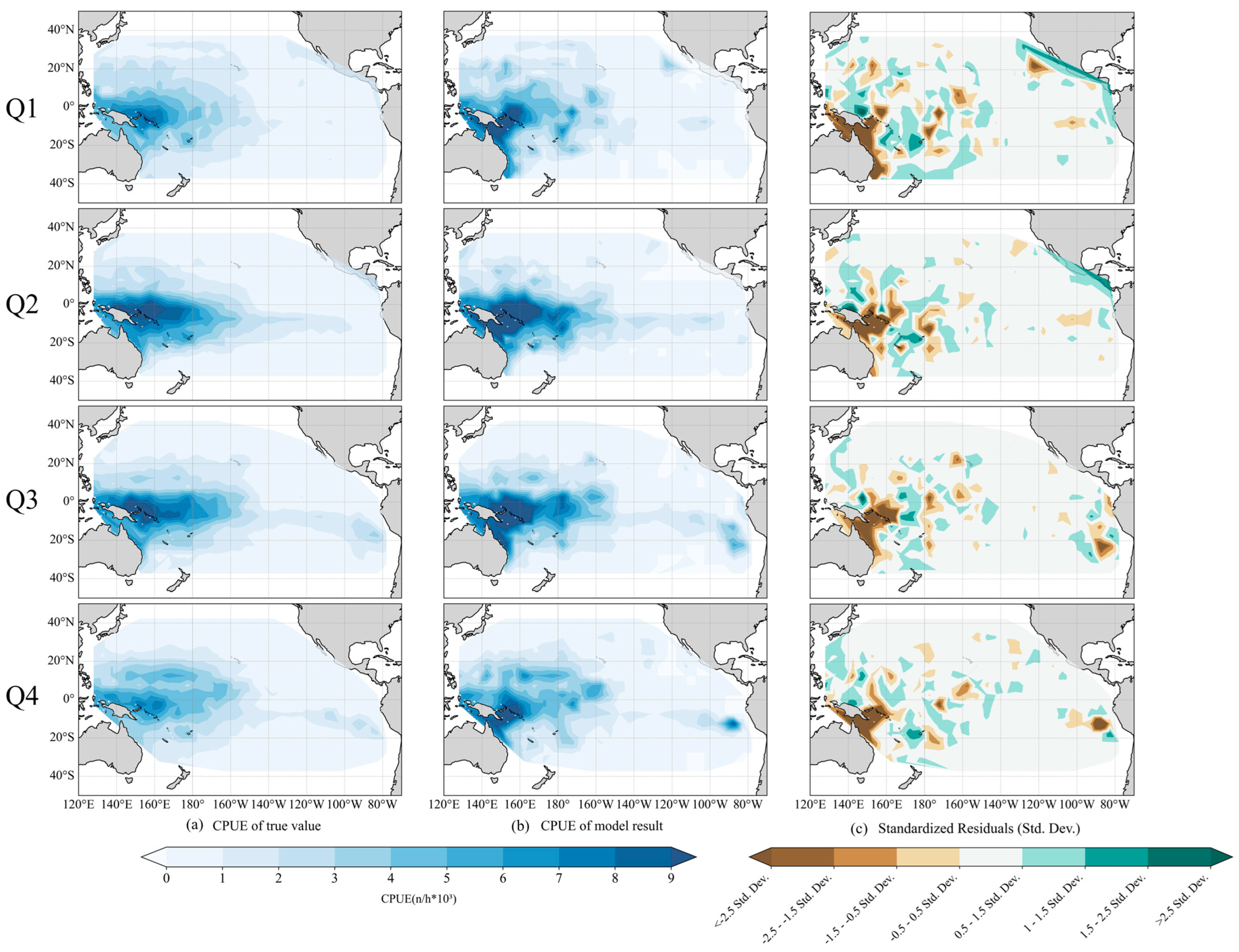
Figure 2 presents the true CPUE values, the model results, and the distribution of standardized residuals for each of the four quarters. The results were linearly interpolated to fill in missing data points and ensure spatial continuity. Figure 2a,b demonstrate that the CPUE of yellowfin tuna displays clear spatial clustering patterns throughout all quarters, with the distribution trends of the model-fitted results closely aligning with the true values. The spatial distribution indicates that regions with elevated CPUE values are primarily found in the Western and Central Pacific Ocean. The boundary between high and low CPUE values roughly follows 150° W longitude, with high-value zones primarily concentrated within the range of 130° E to 150° W and 20° S to 20° N.
Meanwhile, this study analyzed the standardized residuals from the GRF model to enhance the understanding of its handling of spatial heterogeneity. The analysis included both visual inspection (Figure 2c) and quantitative assessment (Table 5). The distribution of standardized residuals is largely uniform across most regions, suggesting that the GRF model effectively addresses spatial heterogeneity in the CPUE of yellowfin tuna throughout the majority of the study area.

3.3. Exploring Key Factors Based on GeoShapley Explainable Method

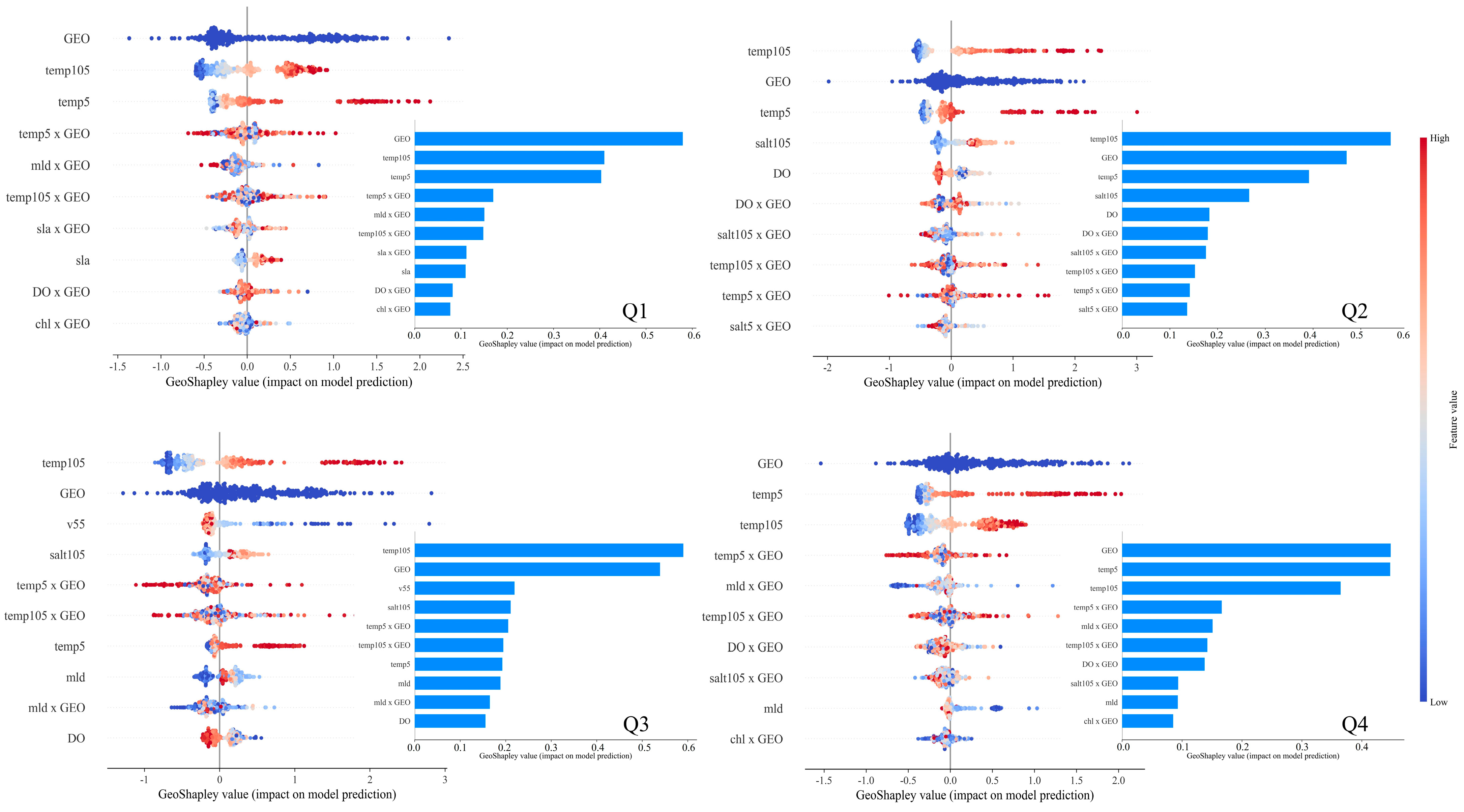
The GeoShapley explainable method was utilized to clarify the model’s global results, focusing on identifying the environmental factors that significantly influence the CPUE of yellowfin tuna. Figure 3 presents a summary and ranking plot of the factors based on the global fitting results of the GRF model. Additionally, to gain a clearer understanding of the GeoShapley values across different quarters, a quantitative analysis was conducted, and the results are tabulated in Table 6.
The global interpretation plot visualizes the influence of each environmental factor on the model’s output. In this plot, each point represents a sample, with denser clustering indicating a higher concentration of samples in that region. The X-axis position of a point is determined by the GeoShapley value of the corresponding feature, which reflects the magnitude of that feature’s impact on the outcome. Points located farther from the central line (zero point) signify a greater influence of the feature on the model’s output—positive GeoShapley values denote a positive impact, while negative values indicate a negative impact. The color of the points, blue or red, represents the magnitude of the feature’s sample values, with blue indicating smaller values and red indicating larger values. In this context, the blue color in “Geo” signifies the positional factor rather than the numerical size. The absolute value interpretation plot, on the other hand, provides a clearer depiction of the degree of influence that each environmental factor has on the CPUE of yellowfin tuna.
The analysis of Figure 3 and Table 6 indicates that, in all quarters, the individual effects of the sea surface temperature and temperature at a 105 m depth, along with the primary spatial effect (GEO), significantly influence the CPUE of yellowfin tuna. Generally, higher temperature values tend to enhance the CPUE, while lower values exert a suppressive effect. Additionally, the interaction between temperature and spatial factors significantly influences the CPUE. For example, during Q1, the interaction between temp5 and spatial factors can lead to a maximum decrease of 0.69 in the CPUE or a maximum increase of 1.72. In Q3, this interaction can result in a maximum decrease of 1.11 or a maximum increase of 1.09 in the CPUE. The importance of these interactions varies across different quarters.
This study prioritizes the exploration of factors and interactions with relatively high absolute average GeoShapley values, as these indicate a more substantial and consistent influence on the CPUE. While certain factors or interactions may display specific patterns of influence in particular quarters, low absolute average GeoShapley values indicate that their overall effect is not significant. Therefore, in our analysis, we focus on those factors and interactions that consistently demonstrate a strong impact on the CPUE, as evidenced by their higher absolute average GeoShapley values.

3.3.1. Individual Effects of Environmental Factors on Yellowfin Tuna Fishery Resources

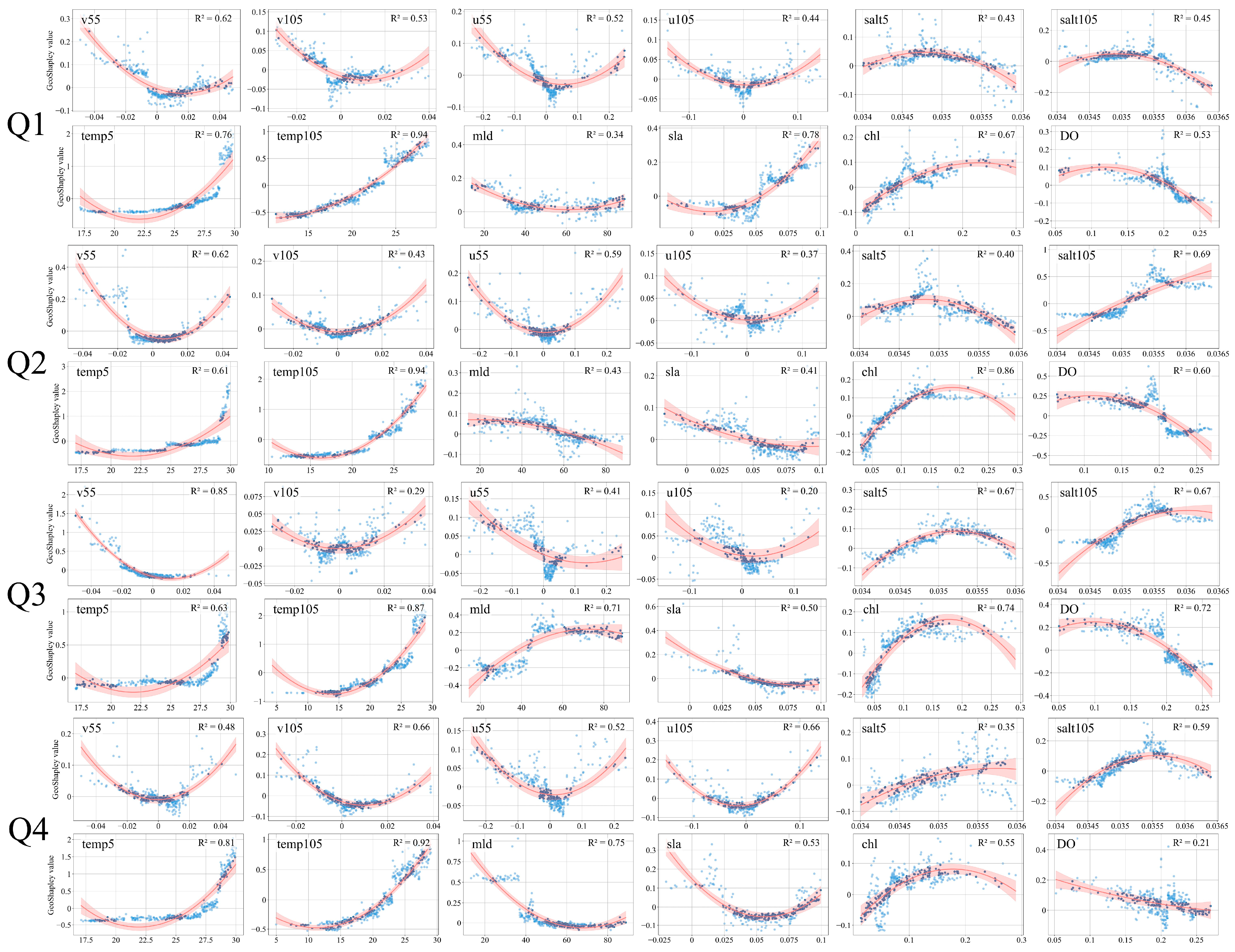
Figure 4 illustrates the marginal contributions of individual environmental factors to the CPUE of yellowfin tuna, with all other factors held constant. This figure illustrates the independent effects of each environmental factor on the CPUE. To better understand the trends in these marginal contributions, a quadratic linear fit was applied to the results of the individual environmental factor effects, accompanied by 95% confidence intervals. These intervals help to clarify the impact of each environmental factor on the CPUE and how their relationships are formed. The R2 values from the quadratic fits indicate a good fit for the data. It is evident from the analysis that, across all four quarters, the relationships between nearly all environmental factors and the yellowfin tuna CPUE exhibit non-linear patterns. The trends in the influences of these factors across various quarters exhibit notable consistency. This study places particular emphasis on examining the individual effects of environmental factors that rank highly in the overall analysis, as these factors are likely to have the most significant impact on the CPUE.
The data indicate that both the sea surface temperature and temperature at a 105 m depth, recognized as significant factors throughout all four quarters, demonstrate a trend in which the GeoShapley value progressively becomes more positive with increasing temperatures. For temp5, temperatures below 27.5 °C exert a consistently negative influence on the CPUE. When the temperature increases from 27.5 °C to 30 °C, it exerts a significant positive effect on the CPUE. For temp105, 22.5 °C serves as a dividing line, where the GeoShapley value changes from negative to positive, and, thereafter, it has a relatively strong positive influence when the temperature exceeds 22.5 °C. Regarding other factors, their importance varies across different quarters. For instance, salt105 and DO exhibit significant marginal effects in Q2 and Q3. In these quarters, when the salinity reaches 35.1 PSU, the GeoShapley value turns positive, reaching its peak at 35.5 PSU, indicating a general trend where the GeoShapley value becomes more positive as the salinity at a 105 m depth increases. Conversely, the dissolved oxygen concentration shows a negative relationship with the GeoShapley value, turning negative at 0.2 mol/m3. Additionally, mld has a relatively significant marginal effect in Q3. In this quarter, when mld reaches 50 m, the GeoShapley value turns positive, peaking at 75 m, and then gradually stabilizes in the positive region, with the GeoShapley value also approaching zero.

3.3.2. Results Regarding Combined Effects of Environmental Factors and Spatial Effects on Yellowfin Tuna Fishery Resources

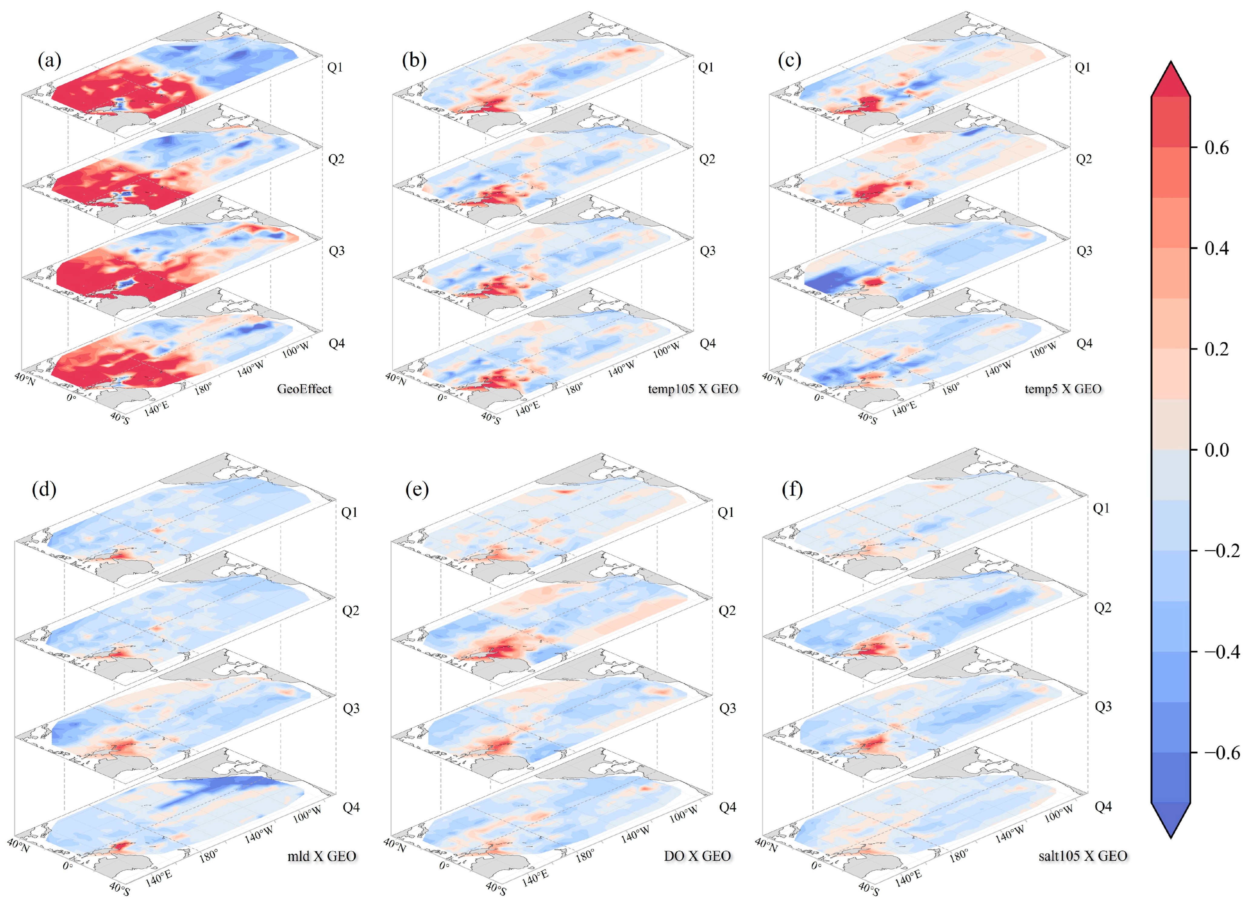
To further elucidate the interaction between the spatial scale location and environmental factors on the yellowfin tuna CPUE, this study presents the spatial distribution of the GeoShapley values for the relevant interactions, as shown in Figure 5. The red regions in the figure indicate positive effects, while the blue regions indicate negative effects. Table 6 illustrates that environmental factors related to main and joint spatial effects significantly influence the yellowfin tuna CPUE across different quarters.
Overall, the main spatial effect (GEO) and the interaction between temperature and location factors are relatively important in all four quarters, while some interaction effects vary in importance across quarters, similarly to the individual effects. The interaction between mld and location has a relatively important impact in Q1, Q3, and Q4; the interaction between DO and location has a relatively important impact in Q2 and Q4; and the interaction between salt105 and location is only relatively important in Q2.
This study found that, across all quarters, the Geoshapley values of the main spatial effect GEO exhibit significant spatial heterogeneity. High-value regions (areas with a positive impact on CPUE) are predominantly concentrated in the Central and Western Pacific Ocean, exhibiting an east–west distribution. The spatial effect exhibits a gradual increase from east to west, whereas the north–south effect is comparatively weaker. The spatial effects of positive and negative impacts are generally demarcated by the 150° W meridian (see Figure 5a); the interaction effect between temp105 and location exhibits similar distribution patterns across the four quarters and also exhibits spatial heterogeneity, as shown in Figure 5b. Overall, both high and low values exhibit small-scale clustering. In the region between 30° S and 10° N, delineated by the 150° W meridian, the western area exhibits a concentration of high values, whereas the eastern area is marked by a concentration of low values. The interaction effect between temp5 and location demonstrates significant spatial heterogeneity during Q1 and Q2, as shown in Figure 5c. The distribution patterns in these two quarters are relatively similar, with three regions of high-value clustering, roughly located between 140°~180° E and 0°~20° S, 120°~150° W and 20°~40° N, and 80°~150° W and 30°~40° S, respectively. In contrast, during Q3 and Q4, negative impacts dominate across the study area, with only small pockets of high-value regions. The interaction between mld and location primarily shows negative impacts across the region, without significant regional variations, as illustrated in Figure 5d. The interaction between DO and location exhibits clear east–west spatial heterogeneity bounded by the 180° meridian in both Q2 and Q4. In particular, there was notable north–south heterogeneity in the Eastern Pacific region during Q2, as depicted in Figure 5e. The interaction effect between salt105 and location is only notably significant during Q2, where the extent of negative impacts outweighs that of positive impacts, as shown in Figure 5f. In this quarter, there is distinct spatial heterogeneity, with a region of high-value clustering located between 140°~180° E and 0°~20° S.

4. Discussion

4.1. Individual Effects of Environmental Factors on Yellowfin Tuna Fishery Resources

This study utilized the GeoShapley method to identify the significance of location-independent environmental factors, as obtained from the GRF method, in each quarter, along with the specific thresholds and marginal relationships affecting the CPUE, as shown in Figure 4. The analysis of individual effects focuses exclusively on the impact of including or excluding each environmental factor on the model outcomes, disregarding the role of spatial effects [29,37]. This enables a specific investigation into how the physiological adaptability, vertical habitat preference, and ecological behaviors of yellowfin tuna influence the CPUE.
This study found that the surface seawater temperature and seawater temperature at 105 m were the primary environmental factors across all quarters, as illustrated in Figure 3. Yellowfin tuna exhibit vertical movement characteristics [38] and are sensitive to temperature. Previous research indicated that the primary determinants influencing the yellowfin tuna CPUE are the surface temperature and temperature at a depth of 100 m [8], aligning with the findings of this study. Additionally, this study found that the yellowfin tuna CPUE exhibits a positive correlation with the temperatures at depths of 5 m and 105 m. Yellowfin tuna are ectothermic organisms that typically inhabit the upper boundary of the thermocline [39], making them highly sensitive to temperature changes. Elevated sea surface temperatures enhance metabolic rates, improving feeding and swimming abilities, which substantially raises the probability of capture. Research has indicated [40] that yellowfin tuna exhibit a significant increase in metabolic rate within the temperature range of 24 °C to 30 °C, leading to more active feeding, swimming, and predatory behavior. The thermocline attains a significant depth at 105 m. With increasing temperatures, the depth of the thermocline rises, which expands the vertical movement space for tuna and subsequently improves catch rates [41]. Moreover, the position and strength of the thermocline are strongly correlated with changes in the mean depth of the mixed layer (mld). Generally, the thermocline is located below the mixed layer or coincides with its bottom, and the temperature gradient is greatest at the boundary between the two. The shallower the mld, the more pronounced the thermocline and the more intense the temperature change; conversely, a deeper mld may weaken or even temporarily eliminate the thermocline [42].
This study also identified quarterly variations in the mechanisms through which environmental factors influence yellowfin tuna fishery resources. Specifically, salt105, DO, and mld in Q2 and Q3 had relatively significant effects on yellowfin tuna fishery resources (Figure 5). This study determined that the optimal salinity for yellowfin tuna at salt105 is 35.5 psu. Studies indicate that yellowfin tuna favor water layers with salinity levels between 34 and 36 psu [43], generally residing in high-salinity surface waters above the thermocline, at depths of approximately 20 to 100 m.
Furthermore, it was noted that a mixed-layer depth of 50 to 75 m significantly enhanced the CPUE for yellowfin tuna. Mature yellowfin tuna primarily inhabit the mixed layer or are vertically distributed below it [44]. Studies have found that, in the central fishing grounds of the Western and Central Pacific Ocean, yellowfin tuna tend to concentrate around the upper boundary of the thermocline at depths of approximately 90 m [38], which is similar to the finding in this study that a mixed-layer depth of around 75 m has the most significant promoting effect on the CPUE. From Q2 to Q3, the intensification of solar radiation gradually increases the sea surface temperature, resulting in the peak metabolic rate in yellowfin tuna [45]. During this period, the mixed-layer depth gradually shallows. This change reduces the energy consumption of tuna diving into cold-water zones, prompting them to stay above the thermocline for feeding, while restricting the upwelling of nutrients. Variations in salinity also alter the osmotic pressure environment of plankton [46], causing them to gather closer to the surface. Yellowfin tuna primarily prey on small fish that feed on plankton, so, in areas with high plankton concentrations, a highly productive ecosystem is formed, with each trophic level supporting the next, forcing the tuna to rise to the surface to feed. Meanwhile, the dissolved oxygen in the subsurface layer further decreases, compressing the living space of tuna [47] and leading to more distinct aggregation patterns. This makes it easier for fishing operations such as longline fishing to catch yellowfin tuna. In addition, the synergistic effects among environmental factors also have an impact. The simultaneous decrease in temperature and dissolved oxygen creates a complex influence on yellowfin tuna, potentially limiting their vertical movement range [48]; the coupling effect of a lower salinity gradient and a low-oxygen environment further compresses the living space of yellowfin tuna [49].

4.2. Impact of Spatial and Environmental Interactions on Yellowfin Tuna Fishery Resources

This study used the GeoShapley method to find that the main spatial effect GEO had a very significant impact on yellowfin tuna fishery resources in each quarter. The interaction between environmental factors and location, which are joint spatial effects, also had varying degrees of impact on yellowfin tuna fishery resources.
Figure 2a,b illustrate significant spatial heterogeneity in the distribution of yellowfin tuna fishery resources. The regions of positive and negative influence of the main spatial effect GEO, indicated in Figure 5a, are delineated by 150° W, paralleling the east–west boundary between high and low CPUE values illustrated in Figure 2b. This boundary also coincides with the demarcation between the Western and Central Pacific Ocean and the Eastern Pacific Ocean. The emergence of this spatial heterogeneity is closely related to the “warm pool”–“cold tongue” phenomenon in the Pacific Ocean. The largest “warm pool” on Earth is located in the tropical waters of the Pacific Ocean. The relatively stable warm-water environment provides a suitable habitat for thermophilic yellowfin tuna [50,51], facilitating their aggregation. Conversely, in the Eastern Pacific Ocean, the Peru Current and equatorial upwelling significantly influence cold upwelling’s dominance [52]. This results in lower surface water temperatures in the region, forming the “cold tongue” and thus restricting the distribution range of yellowfin tuna and causing their populations to be more dispersed [53]. Meanwhile, yellowfin tuna is the primary target species for longline fishing within Exclusive Economic Zones (EEZs) [54]. In contrast to the Eastern Pacific Ocean, the EEZs of Pacific Island nations in the Western and Central Pacific Ocean contain some of the most abundant tuna fishing areas worldwide, drawing numerous foreign fishing vessels for operations in this region [55]. The seabed topography also contributes to this east–west spatial heterogeneity in distribution. Research has indicated that seamount features in the Pacific Ocean affect longline fishing operations aimed at yellowfin tuna [56]. Seamounts and their surrounding waters exhibit higher productivity, which attracts yellowfin tuna to aggregate and feed in these areas [57]. Approximately 50% of the world’s seamounts are distributed in the Western and Central Pacific Ocean [58], particularly within the EEZs of Pacific Island countries. The presence of seamounts has a positive impact on the catch of yellowfin tuna in longline fishing [59]. In contrast, the Eastern Pacific Ocean contains a comparatively lower number of seamounts [60].
In this research, seasonal fluctuations were identified in the interaction effects between environmental factors and location. The interaction effects between the sea surface temperature, the temperature at 105 m, and location had notably significant impacts on yellowfin tuna fishery resources in every quarter. Additionally, the interaction effects of mld, DO, salt105, and location also varied in their influence across different quarters.
Figure 5b,c illustrate that the positive and negative influence trends of the interaction effects between temperature and space mirror the distribution pattern of the “warm pool”–“cold tongue”. Compared to temp5, temp105 shows a higher degree of similarity and more stable seasonal variations. At a depth of 105 m, the water has reached the shallow thermocline. Although there are seasonal changes in its thickness, it is less affected by surface disturbances. In contrast, the 5 m depth is directly influenced by the sea surface, resulting in poorer stability. Moreover, ENSO events have a more direct impact on the surface layer, and their transmission to the shallow thermocline exhibits a lag effect [61]. From Q3 to Q4, the negative influence range of temp5 expanded within the study area. During this period, the seasonal upwelling along the Peru–Chile coast intensified, typically bringing in nutrient-rich cold water. Super El Niño events occurring during the study period may have inhibited upwelling and decreased nutrient inputs [62], which may have led to a decline in the CPUE for yellowfin tuna from east to west. As shown in Figure 5d, the interaction effect between mld and location was only insignificant in Q2. Within the tropical Pacific, the mld is subject to the influence of salinity stratification, resulting in relatively weak seasonal variations [63]. Meanwhile, the negative influence is quite pronounced across the study area. The depth of the mixed layer affects the distribution and transport of nutrients [64]. A shallower mixed-layer depth is conducive to confining yellowfin tuna in the upper water layer, thereby increasing their catchability [65]. Horizontal ocean currents (such as the Equatorial Current and eddies) alter the spatial pattern of the mixed-layer depth through advection. Warm eddies cause the mixed-layer depth to shallow, while cold eddies cause it to deepen. This spatial heterogeneity forces tuna to migrate frequently, increasing their energy expenditure and dispersing the population density [66]. Figure 5e reveals that the dissolved oxygen concentration exhibits a significant interaction effect with location. Yellowfin tuna display hypoxic avoidance behavior, tending to aggregate in oxygen-rich areas [65]. Influenced by monsoon transitions and the “warm pool”–“cold tongue” phenomenon, water stratification is more pronounced in summer than in winter, leading to seasonal differences in the distribution of dissolved oxygen [67]. During Q2, the spatial heterogeneity of the north–south interaction effect in the Eastern Pacific Ocean may be attributed to the fact that, during this period, the northern waters had sufficient dissolved oxygen content, which promoted the vertical aggregation of fish and thereby increased the CPUE. Near the equator, the oxygen minimum zone caused a decrease in dissolved oxygen levels in the midwater layer, compressing the fish habitat layer and leading to a decline in CPUE. In the southern region, upwellings such as the Peru Current caused an increase in dissolved oxygen levels, enhancing fish activity and resulting in another increase in CPUE [68,69,70]. The interaction effect between salinity at 105 m and location is only significant in Q2, as shown in Figure 5f. Salinity fronts formed at the edge of the warm pool attract tuna for feeding, thereby increasing the catch [43]. This is likely due to the sharp changes in salinity gradients caused by rising air temperatures. The effect is not significant in other areas, as salinity does not play a decisive role in fish aggregation. Instead, it needs to interact with other environmental factors to influence the distribution of fishery resources [71].

4.3. Application of GRF Combined with the Geoshapley Method in Yellowfin Tuna Resource Research

This study employed the GRF method to model the relationship between the quarterly CPUE of yellowfin tuna and environmental factors and compared it with traditional RF and XGBRF methods. Table 4 shows that GRF demonstrated higher R2 values and lower MAE and RMSE values across all quarters, outperforming other methods in predictive performance. The model simulation results align with the trends observed in actual data, further validating its effectiveness. Subsequently, the GRF output results were input into the GeoShapley model to enable joint spatial effect interpretation.
The traditional random forest model, due to its strong resistance to overfitting and its robustness, has been widely applied in previous studies on tuna resources, with many studies indicating favorable prediction outcomes [19,20,72]. Subsequently, in order to further enhance the prediction accuracy, researchers proposed extreme gradient boosting random forest (XGBRF) by combining the traditional random forest method with extreme gradient boosting. This method significantly enhances the learning efficiency and model flexibility by incorporating random sampling and random feature selection, which further improves the prediction accuracy [21]. However, these methods are based on global fitting and struggle to adequately address spatial heterogeneity between different sea areas.
Considering that the study area covers most of the Pacific Ocean, where environmental factors (such as sea surface temperature, salinity, and primary productivity) exhibit significant spatial variability (see Figure 5a), GRF introduces spatially adaptive bandwidth and local weights to partition the region and construct customized local models, thereby more effectively mitigating the impact of spatial heterogeneity (Figure 2c). Compared to global modeling, GRF more precisely captures the relationship between the CPUE and environmental factors across regions, enhancing model reliability.
Simultaneously, numerous studies have employed the SHAP method to elucidate the contributions of outcomes from “black box” machine learning models, with applications already noted in fishery resource research [26,27,73]. The SHAP explainable method overlooks the influence of spatial effects on the model’s output results. Given that yellowfin tuna are migratory fish with periodic movement patterns [1], there are variations in marine environments across different geographical locations. Additionally, spatial effects, including location factors, can influence the impacts of environmental factors on yellowfin tuna fishery resources. The GeoShapley method addresses the spatial limitations of SHAP, revealing both the independent effects of environmental factors on the CPUE and their interactions with spatial location, thereby providing a more comprehensive understanding of the coupling mechanisms between yellowfin tuna and environmental factors.
Based on this, for the study of highly ocean environment-sensitive migratory fishery resources like yellowfin tuna, it is imperative to incorporate spatial heterogeneity and the impact of spatial effects into our research considerations. This study is the first to introduce the GRF model, which accounts for spatial influence differences, in conjunction with the GeoShapley explainable method, into the research of yellowfin tuna fishery resources. The aim was to identify environmental factors that have significant impacts on yellowfin tuna fishery resources under different contexts and their modes of action. Through spatial explicit modeling, we validated the overall impacts of environmental factors and revealed regional specificity patterns that are difficult to capture using traditional non-spatial methods. Management can utilize GRF in combination with the GeoShapley method to accurately identify the impacts of key environmental factors on the yellowfin tuna CPUE in different geographical areas, thereby promoting a transition from “uniform static management” to “regionalized, indicator-driven dynamic management” and achieving more scientific, ecological, and sustainable fishery regulation.
Although the GRF method can make predictions under spatially heterogeneous conditions and performs well compared to traditional machine learning methods, it still has limitations. Future research could combine methods that account for spatial heterogeneity (such as GWR, MGWR, and GTWR) with other machine learning methods and apply them to fishery resource research to more accurately capture local patterns and improve the predictive performance. Additionally, the GRF method may overlook the impact of uneven sampling densities on the model, particularly the local fitting bias caused by low-catch areas. Future research could integrate scientific survey data, design sensitivity tests, and quantify the effects of sampling density changes on model stability. Furthermore, the current study has not conducted a sensitivity analysis or cross-validation on hyperparameters such as λ and α in the GRF model. Future research could introduce relevant methods to enhance the transparency and reproducibility of the hyperparameter selection process. In addition, as a spatial extension of the SHAP explainable method, the GeoShapley method acknowledges the interaction between spatial and factor variables; however, it neglects the interactions among environmental factors and the more profound interactions between spatial and environmental factors. In future research, more in-depth interaction patterns can be introduced into the GeoShapley explainable method to further improve the explainable model framework.

5. Conclusions and Prospects

This study innovatively combines the geographical random forest (GRF) model with the GeoShapley explainable analysis method to explore the relationship between the distribution of a highly migratory species, the Pacific yellowfin tuna (Thunnus albacares), and environmental factors. The research results indicate that (1) the GRF model significantly outperforms traditional random forest and extreme gradient boosting (XGBoost) models in predictive performance and effectively addresses the spatial heterogeneity issues within the study area; (2) the GeoShapley method overcomes the limitations of traditional SHAP methods, enabling, for the first time, an analysis of the complex relationship between environmental factors and fishery resource distribution from the perspective of spatial effects. Through multi-seasonal analysis, this study not only quantified the individual effects of key environmental factors but also revealed their interaction mechanisms with the spatial location, providing new theoretical insights into the spatiotemporal distribution patterns of yellowfin tuna fishery resources.
This study exhibits a certain degree of bias in the selection of environmental factors. Although variance inflation factor (VIF) screening can eliminate multicollinearity to ensure model fitting performance, this process may also exclude environmental factors that significantly influence the results, thereby affecting subsequent research. Based on this, future research could explore new methods of selecting environmental factors and combine them with other models and machine learning methods that account for spatial heterogeneity to investigate the underlying effects of different environmental factors on the results under spatial effects. Additionally, the impact of spatial scale issues and potential confounding factors is a key challenge in large-scale marine research, where spatial heterogeneity, such as the complex distribution of the sea surface temperature, plays a significant role. This study reduced seasonal interference by dividing the data into quarters, but this treatment may have exacerbated spatial confounding effects. In future research, integrating seasonal and spatial joint models may allow researchers to more effectively analyze these effects. Future research can focus on optimizing the following aspects: (1) establishing spatiotemporal joint modeling to test mixed-effects models such as spatiotemporal interaction terms, explicitly distinguishing seasonal and spatial effects; (2) data augmentation by integrating additional physical and chemical variables (e.g., temperature–salinity profiles, ocean current data) to control for potential confounding factors; (3) conducting sensitivity analyses to validate the robustness of quarterly divisions or exploring dynamic time window divisions.

Author Contributions

Conceptualization, Z.H. and X.Y.; methodology, M.L.; software, S.F.; validation, Z.H., X.Y. and J.Z.; formal analysis, X.Y.; investigation, Z.H.; resources, J.Z.; data curation, S.F.; writing—original draft preparation, Z.H.; writing—review and editing, Z.H.; visualization, Z.H.; supervision, X.Y.; project administration, X.Y.; funding acquisition, J.Z. All authors have read and agreed to the published version of the manuscript.

Funding

This research was funded by the National Key Research and Development Program of China (2024YFD2400603).

Institutional Review Board Statement

Not applicable.

Data Availability Statement

The data that support the findings of this study are available from the corresponding author upon reasonable request.

Acknowledgments

This project was funded in part by the National Key Research and Development Program of China. We thank all our colleagues from the Research Laboratory for their work during data collection.

Conflicts of Interest

The authors declare no conflicts of interest.

Appendix A

Appendix A.1

This study used the seaborn package in Python 3.9.2 to calculate the Pearson correlation coefficients between various environmental factors, as shown in Figure A1. It can be seen that there are significant correlations between temperature and salinity in different water layers, especially between adjacent water layers, indicating that the environmental factors temp5, temp105, salt5, and salt105 retained in the VIF test in this study can also represent the environmental factors of adjacent water layers to a certain extent.
Figure A1. Heat map showing correlations between environmental factors in each quarter.
Fishes 10 00417 g0a1

References

  1. Schaefer, K.M.; Fuller, D.W.; Block, B.A. Movements, Behavior, and Habitat Utilization of Yellowfin Tuna (Thunnus albacares) in the Northeastern Pacific Ocean, Ascertained through Archival Tag Data. Mar. Biol. 2007, 152, 503–525. [Google Scholar] [CrossRef]
  2. Collette, B.B.; Reeb, C.; Block, B.A. Systematics of the Tunas and Mackerels (Scombridae); Academic Press: New York, NY, USA, 2001; pp. 1–33. [Google Scholar]
  3. Hare, S.R.; Williams, P.G.; Jordán, C.C.; Hamer, P.A.; Hampton, W.J.; Lehodey, P.; Macdonald, M.; Scott, R.D.; Phillips, J.S.; Senina, I.; et al. The Western and Central Pacific Tuna Fishery: 2021 Overview and Status of Stocks; SPC Tuna Fisheries Assesstent Report No. 22; Pacific Community: Noumea, New Caledonia, 2022. [Google Scholar]
  4. FAO. The State of World Fisheries and Aquaculture 2024; FAO: Rome, Italy, 2024. [Google Scholar]
  5. Tomczak, M.; Godfrey, J.S. Regional Oceanography: An Introduction; Elsevier: Amsterdam, The Netherlands, 2013. [Google Scholar]
  6. Lehodey, P.; Andre, J.-M.; Bertignac, M.; Hampton, J.; Stoens, A.; Menkes, C.; Memery, L.; Grima, N. Predicting Skipjack Tuna Forage Distributions in the Equatorial Pacific Using a Coupled Dynamical Bio-Geochemical Model. Fish. Oceanogr. 1998, 7, 317–325. [Google Scholar] [CrossRef]
  7. Fischer, E.M.; Bador, M.; Huser, R.; Kendon, E.J.; Robinson, A.; Sippel, S. Record-Breaking Extremes in a Warming Climate. Nat. Rev. Earth. Environ. 2025, 6, 456–470. [Google Scholar] [CrossRef]
  8. Li, D.X.; Zou, X.R.; Zhou, S.T. Spatio-temporal distribution of Thunnus albacares CPUE and its relationship with environmental factors in central Pacific Ocean. South China Fish. Sci. 2024, 20, 68–76. (In Chinese) [Google Scholar]
  9. Yen, K.-W.; Wang, G.; Lu, H.-J. Evaluating Habitat Suitability and Relative Abundance of Skipjack (Katsuwonus pelamis) in the Western and Central Pacific during Various El Niño Events. Ocean Coast. Manag. 2017, 139, 153–160. [Google Scholar] [CrossRef]
  10. Puspita, A.R.; Syamsuddin, M.L.; Subiyanto; Syamsudin, F.; Purba, N.P. Predictive Modeling of Eastern Little Tuna (Euthynnus affinis) Catches in the Makassar Strait Using the Generalized Additive Model. J. Mar. Sci. Eng. 2023, 11, 165. [Google Scholar] [CrossRef]
  11. Yang, C.L.; Yang, X.M.; Zhu, J.F. Response of environmental factors to the distribution of tuna purse seine bonito in the western and central Pacific Ocean during different types of ENSO. South China Fish. Sci. 2021, 17, 8–18. (In Chinese) [Google Scholar]
  12. Zheng, H.H.; Yang, X.M.; Zhu, J.F. Environmental impact mechanism of skipjack tuna fishery in Western and Central Pacific Ocean based on Multi-scale Geographical Weighted Regression Model (MGWR). South China Fish. Sci. 2023, 19, 1–10. [Google Scholar]
  13. Li, M.; Yang, X.; Wang, Y.; Wang, Y.; Zhu, J. The Use of the GWPCA-MGWR Model for Studying Spatial Relationships between Environmental Variables and Longline Catches of Yellowfin Tunas. J. Mar. Sci. Eng. 2024, 12, 1002. [Google Scholar] [CrossRef]
  14. Wu, L.; Li, X.; Yuan, J.; Wang, S. Real-time prediction of tunnel face conditions using XGBoost random forest algorithm. Front. Struct. Civ. Eng. 2023, 17, 1777–1795. [Google Scholar] [CrossRef]
  15. Zhang, M.; Song, L.; Pan, C.; Wang, L. Prediction on Yellowfin Tuna (Thunnus albacares) Fishing Ground in Waters near the Marshall Islands Based on SMOTETomek-RF. Fish. Oceanogr. 2025, 34, e12704. [Google Scholar] [CrossRef]
  16. Young, P.; Shellswell, S. Time Series Analysis, Forecasting and Control. IEEE Trans. Autom. Control 1972, 17, 281–283. [Google Scholar] [CrossRef]
  17. Breiman, L. Statistical Modeling: The Two Cultures (with Comments and a Rejoinder by the Author). Statist. Sci. 2001, 16, 199–231. [Google Scholar] [CrossRef]
  18. Fotheringham, A.S.; Yang, W.; Kang, W. Multiscale Geographically Weighted Regression (MGWR). Ann. Am. Assoc. Geogr. 2017, 107, 1247–1265. [Google Scholar] [CrossRef]
  19. Baba, S.; Matsuishi, T. Pacific Saury Fishing Forecasting by Using Random Forest. Nippon Suisan Gakkaishi 2015, 81, 2–9. [Google Scholar] [CrossRef]
  20. Baidai, Y.; Dagorn, L.; Amande, M.J.; Gaertner, D.; Capello, M. Machine Learning for Characterizing Tropical Tuna Aggregations under Drifting Fish Aggregating Devices (DFADs) from Commercial Echosounder Buoys Data. Fish. Res. 2020, 229, 105613. [Google Scholar] [CrossRef]
  21. Zhang, C.; Zhou, W.F.; Tang, F.H. Forecasting model of yellowfin tuna fishing grounds in the central and western Pacific Ocean based on machine learning. Trans. Chin. Soc. Agric. Eng. 2022, 38, 330–338. (In Chinese) [Google Scholar]
  22. Song, L.M.; Ren, S.Y.; Zhang, M.; Sui, H.S. Fishing ground forecasting models for yellowfin tuna (Thunnus albacares) in the tropical waters of the Atlantic Ocean based on ensemble learning. J. Fish. Sci. China 2021, 28, 1069–1078. (In Chinese) [Google Scholar]
  23. Georganos, S.; Grippa, T.; Niang Gadiaga, A.; Linard, C.; Lennert, M.; Vanhuysse, S.; Mboga, N.; Wolff, E.; Kalogirou, S. Geographical Random Forests: A Spatial Extension of the Random Forest Algorithm to Address Spatial Heterogeneity in Remote Sensing and Population Modelling. Geocarto Int. 2021, 36, 121–136. [Google Scholar] [CrossRef]
  24. Georganos, S.; Grippa, T.; Gadiaga, A.; Vanhuysse, S.; Kalogirou, S.; Lennert, M.; Linard, C. An Application of Geographical Random Forests for Population Estimation in Dakar, Senegal Using Very-High-Resolution Satellite Imagery. In Proceedings of the 2019 Joint Urban Remote Sensing Event (Jurse), Vannes, France, 22–24 May 2019. [Google Scholar]
  25. Lotfata, A.; Georganos, S.; Kalogirou, S.; Helbich, M. Ecological Associations between Obesity Prevalence and Neighborhood Determinants Using Spatial Machine Learning in Chicago, Illinois, USA. ISPRS Int. J. Geo-Inf. 2022, 11, 550. [Google Scholar] [CrossRef]
  26. Zhao, Y.; Yuan, H.C. Prediction of Pacific Thunnus alalunga Fishery Based on a Multiple-Channel Single Regression Module with Explainability. Acta Hydrobiol. Sin. 2025, 49, 15–27. (In Chinese) [Google Scholar]
  27. Zhang, T.; Guo, H.; Song, L.; Yuan, H.; Sui, H.; Li, B. Evaluating the Importance of Vertical Environmental Variables for Albacore Fishing Grounds in Tropical Atlantic Ocean Using Machine Learning and Shapley Additive Explanations (SHAP) Approach. Fish. Oceanogr. 2025, 34, e12701. [Google Scholar] [CrossRef]
  28. Lan, K.-W.; Lee, M.-A.; Nishida, T.; Lu, H.-J.; Weng, J.-S.; Chang, Y. Environmental Effects on Yellowfin Tuna Catch by the Taiwan Longline Fishery in the Arabian Sea. Int. J. Remote Sens. 2012, 33, 7491–7506. [Google Scholar] [CrossRef]
  29. Li, Z. GeoShapley: A Game Theory Approach to Measuring Spatial Effects in Machine Learning Models. Ann. Am. Assoc. Geogr. 2024, 114, 1365–1385. [Google Scholar] [CrossRef]
  30. Hilborn, R.; Walters, C.J. Quantitative Fisheries Stock Assessment: Choice, Dynamics and Uncertainty, 1st ed.; Springer: New York, NY, USA, 1992. [Google Scholar]
  31. Ortiz, M. Standardized Catch Rates for Yellowfin Tuna (Thunnus albacares) from the US Pelagic Longline Fleet. Col. Vol. Sci. Pap. ICCAT 2004, 56, 660–675. Available online: https://www.iccat.int/Documents/CVSP/CV056_2004/n_2/CV056020660.pdf (accessed on 8 August 2025).
  32. Kuhn, M. Applied Predictive Modeling; Springer: New York, NY, USA, 2013. [Google Scholar]
  33. Breiman, L. Random Forests. Mach. Learn. 2001, 45, 5–32. [Google Scholar] [CrossRef]
  34. Zhang, H.; Wan, L.; Li, Y. Prediction of Soil Organic Carbon Content Using Sentinel-1/2 and Machine Learning Algorithms in Swamp Wetlands in Northeast China. IEEE J. Sel. Top. Appl. Earth Observ. Remote Sens. 2023, 16, 5219–5230. [Google Scholar] [CrossRef]
  35. Sun, K.; Zhou, R.Z.; Kim, J.; Hu, Y. PyGRF: An Improved Python Geographical Random Forest Model and Case Studies in Public Health and Natural Disasters. In Transactions in GIS; John Wiley & Sons: Hoboken, NJ, USA, 2024. [Google Scholar]
  36. Quiñones, S.; Goyal, A.; Ahmed, Z.U. Geographically Weighted Machine Learning Model for Untangling Spatial Heterogeneity of Type 2 Diabetes Mellitus (T2D) Prevalence in the USA. Sci. Rep. 2021, 11, 6955. [Google Scholar] [PubMed]
  37. Peng, Z.; Ji, H.; Yuan, R.; Wang, Y.; Easa, S.M.; Wang, C.; Cui, H.; Zhao, X. Modeling and Spatial Analysis of Heavy-Duty Truck CO2 Using Travel Activities. J. Transp. Geogr. 2025, 124, 104158. [Google Scholar] [CrossRef]
  38. Yang, S.L. The Influence of Subsurface Environment on the Vertical Water Column Distribution and Longline Fishing Catch Rate of Yellowfin Tuna in Tropical Central Western Pacific. Ph.D. Thesis, Shanghai Ocean University, Shanghai, China, 2020. (In Chinese). [Google Scholar]
  39. Brill, R.W. Understanding Environmental Influences on Movements and Depth Distributions of Tunas and Billfishes Can Significantly Improve Population Assessments. Am. Fish. Soc. Symp. 2001, 25, 179–198. [Google Scholar]
  40. Brill, R.W. A Review of Temperature and Oxygen Tolerance Studies of Tunas Pertinent to Fisheries Oceanography, Movement Models and Stock Assessments. Fish. Oceanogr. 1994, 3, 204–216. [Google Scholar] [CrossRef]
  41. Fuller, D.W.; Schaefer, K.M.; Hampton, J.; Caillot, S.; Leroy, B.M.; Itano, D.G. Vertical Movements, Behavior, and Habitat of Bigeye Tuna (Thunnus obesus) in the Equatorial Central Pacific Ocean. Fish. Res. 2015, 172, 57–70. [Google Scholar] [CrossRef]
  42. de Boyer Montégut, C.; Madec, G.; Fischer, A.S.; Lazar, A.; Iudicone, D. Mixed Layer Depth over the Global Ocean: An Examination of Profile Data and a Profile-Based Climatology. J. Geophys. Res. 2004, 109, C12003. [Google Scholar] [CrossRef]
  43. Arrizabalaga, H.; Dufour, F.; Kell, L.; Merino, G.; Ibaibarriaga, L.; Chust, G.; Irigoien, X.; Santiago, J.; Murua, H.; Fraile, I.; et al. Global Habitat Preferences of Commercially Valuable Tuna. Deep Sea Res. Part II Top. Stud. Oceanogr. 2015, 113, 102–112. [Google Scholar] [CrossRef]
  44. Block, B.A.; Keen, J.E.; Castillo, B.; Dewar, H.; Freund, E.V.; Marcinek, D.J.; Brill, R.W.; Farwell, C. Environmental Preferences of Yellowfin Tuna (Thunnus albacares) at the Northern Extent of Its Range. Mar. Biol. 1997, 130, 119–132. [Google Scholar] [CrossRef]
  45. Klinger, D.H.; Dale, J.J.; Gleiss, A.C.; Brandt, T.; Estess, E.E.; Gardner, L.; Machado, B.; Norton, A.; Rodriguez, L.; Stiltner, J.; et al. The Effect of Temperature on Postprandial Metabolism of Yellowfin Tuna (Thunnus albacares). Comp. Biochem. Physiol. A Mol. Integr. Physiol. 2016, 195, 32–38. [Google Scholar] [CrossRef]
  46. Bœuf, G.; Payan, P. How Should Salinity Influence Fish Growth? Comp. Biochem. Physiol. Part C Toxicol. Pharmacol. 2001, 130, 411–423. [Google Scholar] [CrossRef]
  47. Fiedler, P.C.; Talley, L.D. Hydrography of the Eastern Tropical Pacific: A Review. Prog. Oceanogr. 2006, 69, 143–180. [Google Scholar] [CrossRef]
  48. Bernal, D.; Brill, R.W.; Dickson, K.A.; Shiels, H.A. Sharing the Water Column: Physiological Mechanisms Underlying Species-Specific Habitat Use in Tunas. Rev. Fish. Biol. Fish. 2017, 27, 843–880. [Google Scholar] [CrossRef]
  49. Bertrand, A.; Bard, F.-X.; Josse, E. Tuna Food Habits Related to the Micronekton Distribution in French Polynesia. Mar. Biol. 2002, 140, 1023–1037. [Google Scholar] [CrossRef]
  50. Lehodey, P.; Bertignac, M.; Hampton, J.; Lewis, A.; Picaut, J. El Niño Southern Oscillation and Tuna in the Western Pacific. Nature 1997, 389, 715–718. [Google Scholar] [CrossRef]
  51. Lan, K.-W.; Shimada, T.; Lee, M.-A.; Su, N.-J.; Chang, Y. Using Remote-Sensing Environmental and Fishery Data to Map Potential Yellowfin Tuna Habitats in the Tropical Pacific Ocean. Remote Sens. 2017, 9, 444. [Google Scholar] [CrossRef]
  52. Lv, J.-M.; Ju, J.-H.; Zhang, Q.-Y.; Tao, S.-Y. The characteristics of ENSO cycle in different phases of pacific decadal oscillation. Clim. Environ. Res. 2005, 10, 238–249. [Google Scholar]
  53. Prince, E.D.; Goodyear, C.P. Hypoxia-Based Habitat Compression of Tropical Pelagic Fishes. Fish. Oceanogr. 2006, 15, 451–464. [Google Scholar] [CrossRef]
  54. Fonteneau, A.; Chassot, E.; Bodin, N. Global Spatio-Temporal Patterns in Tropical Tuna Purse Seine Fisheries on Drifting Fish Aggregating Devices (DFADs): Taking a Historical Perspective to Inform Current Challenges. Aquat. Living Resour. 2013, 26, 37–48. [Google Scholar] [CrossRef]
  55. Miller, A.M.; Bush, S.R.; van Zwieten, P.A. Sub-Regionalisation of Fisheries Governance: The Case of the Western and Central Pacific Ocean Tuna Fisheries. Marit. Stud. 2014, 13, 17. [Google Scholar] [CrossRef]
  56. Fei, J.J.; Li, C.; Zhang, J.; Teng, Y.X.; Wu, Y.T.; Shi, J.G. Effects of seamount characteristics in Central and Western Pacific Ocean on CPUEs of yellowfin tuna (Thunnus albacares) in longline and purse seine fisheries. South China Fish. Sci. 2024, 20, 1–10. (In Chinese) [Google Scholar]
  57. Shi, X.F.; Wang, X.; Wang, Y.X.; Shi, J.G.; Zhang, J. Feeding biology of yellowfin tuna (Thunnus albacares) in tropical central and western Pacific Ocean. South China Fish. Sci. 2022, 18, 43–51. (In Chinese) [Google Scholar]
  58. Deary, A.L.; Moret-Ferguson, S.; Engels, M.; Zettler, E.; Jaroslow, G.; Sancho, G. Influence of Central Pacific Oceanographic Conditions on the Potential Vertical Habitat of Four Tropical Tuna Species. Pac. Sci. 2015, 69, 461. [Google Scholar] [CrossRef]
  59. Morato, T.; Hoyle, S.D.; Allain, V.; Nicol, S.J. Tuna Longline Fishing around West and Central Pacific Seamounts. PLoS ONE 2010, 5, e14453. [Google Scholar] [CrossRef]
  60. Yesson, C.; Letessier, T.B.; Nimmo-Smith, A.; Hosegood, P.; Brierley, A.S.; Hardouin, M.; Proud, R. Improved Bathymetry Leads to 4000 New Seamount Predictions in the Global Ocean. UCL Open Environ. 2021, 3, e030. [Google Scholar] [PubMed]
  61. McPhaden, M.J.; Zhang, D. Slowdown of the Meridional Overturning Circulation in the Upper Pacific Ocean. Nature 2002, 415, 603–608. [Google Scholar] [CrossRef] [PubMed]
  62. Chavez, F.P.; Strutton, P.G.; Friederich, G.E.; Feely, R.A.; Feldman, G.C.; Foley, D.G.; McPhaden, M.J. Biological and Chemical Response of the Equatorial Pacific Ocean to the 1997-98 El Niño. Science 1999, 286, 2126–2131. [Google Scholar] [CrossRef] [PubMed]
  63. Sprintall, J.; Tomczak, M. Evidence of the Barrier Layer in the Surface Layer of the Tropics. J. Geophys. Res. Ocean. 1992, 97, 7305–7316. [Google Scholar] [CrossRef]
  64. Richards, K.J.; Whitt, D.B.; Brett, G.; Bryan, F.O.; Feloy, K.; Long, M.C. The Impact of Climate Change on Ocean Submesoscale Activity. J. Geophys. Res. Ocean. 2021, 126, e2020JC016750. [Google Scholar] [CrossRef]
  65. Hu, C.; Harrison, D.P.; Hinton, M.G.; Siegrist, Z.C.; Kiefer, D.A. Habitat Analysis of the Commercial Tuna of the Eastern Tropical Pacific Ocean. Fish. Oceanogr. 2018, 27, 417–434. [Google Scholar] [CrossRef]
  66. Lan, K.-W.; Evans, K.; Lee, M.-A. Effects of Climate Variability on the Distribution and Fishing Conditions of Yellowfin Tuna (Thunnus albacares) in the Western Indian Ocean. Clim. Change 2013, 119, 63–77. [Google Scholar] [CrossRef]
  67. Stramma, L.; Prince, E.D.; Schmidtko, S.; Luo, J.; Hoolihan, J.P.; Visbeck, M.; Wallace, D.W.R.; Brandt, P.; Körtzinger, A. Expansion of Oxygen Minimum Zones May Reduce Available Habitat for Tropical Pelagic Fishes. Nat. Clim. Change 2012, 2, 33–37. [Google Scholar] [CrossRef]
  68. Mediodia, H.J.; Kahui, V.; Noy, I. Sea Surface Temperature and Tuna Catch in the Eastern Pacific Ocean under Climate Change. Mar. Resour. Econ. 2023, 38, 329–351. [Google Scholar] [CrossRef]
  69. Fonteneau, A.; Ariz, J. Tunas Yield per Recruit and MSY of Longline Fisheries, Case of Yellowfin Stock in the Eastern Pacific Ocean; IATTC: La Jolla, CA, USA, 2011. [Google Scholar]
  70. Vaihola, S.; Kininmonth, S. Environmental Factors Determine Tuna Fishing Vessels’ Behavior in Tonga. Fishes 2023, 8, 602. [Google Scholar] [CrossRef]
  71. Emerson, S.; Watanabe, Y.W.; Ono, T.; Mecking, S. Temporal Trends in Apparent Oxygen Utilization in the Upper Pycnocline of the North Pacific: 1980–2000. J. Oceanogr. 2004, 60, 139. [Google Scholar] [CrossRef]
  72. Chen, X.Z.; Fan, W.; Cui, X.S.; Zhou, W.F.; Tang, F.H. Fishing ground forecasting of Thunnus alalung in Indian Ocean based on random forest. Acta. Oceanol. Sin. 2013, 35, 158–164. [Google Scholar]
  73. Liu, L.; Wan, R.; Wu, F.; Wang, Y.; Zhu, Y.; Zhou, C. An Integrative Machine Learning Approach to Understanding South Pacific Ocean Albacore Tuna Habitat Features. ICES J. Mar. Sci. 2025, 82, fsaf003. [Google Scholar] [CrossRef]
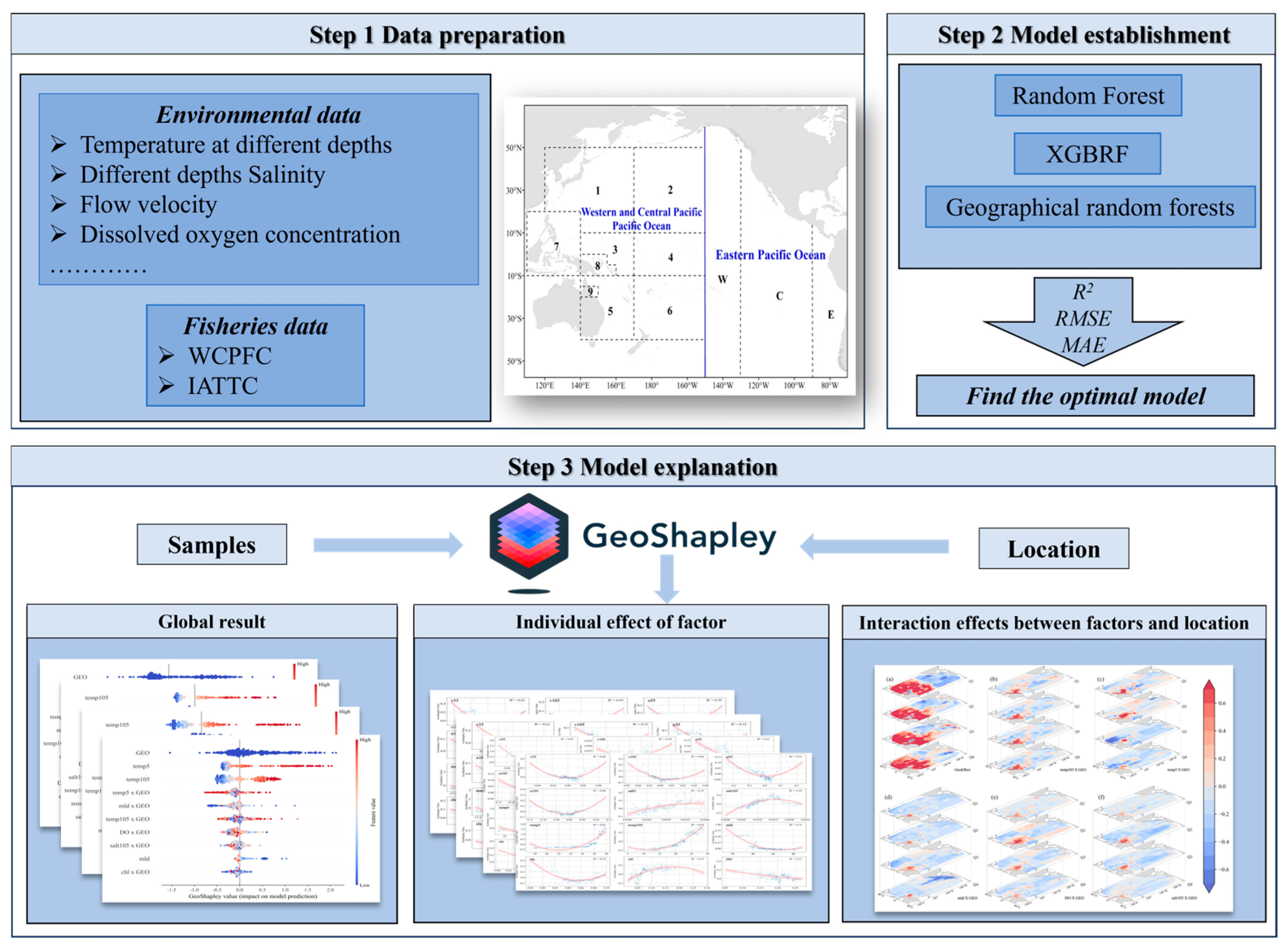
Figure 1. Workflow diagram of the study. (In the zoning map in the first step of data preparation, the numbers represent WCPFC zone labels, while the letters represent IATTC zone labels).
Fishes 10 00417 g001
Figure 2. Distribution of actual values, model outcomes, and standardized residuals in GRF results across various quarters.
Fishes 10 00417 g002
Figure 3. Global interpretation and ranking of environmental factors under the GeoShapley explainable method in different quarters. (The main figure displays the global interpretation results for the top ten highest-ranked factors, as selected through the GeoShapley explanation; the inset in the lower-right corner shows the absolute value interpretation results for these top ten factors based on GeoShapley; “Geo” signifies the positional factor).
Fishes 10 00417 g003
Figure 4. Relationships between environmental factors and individual effects of CPUE on yellowfin tuna.
Fishes 10 00417 g004
Figure 5. Distribution of GeoShapley values for the interaction effects of environmental factors and location on resources in different quarters. ((a) shows the main spatial effect, (bf) show the interaction effects of temperature at 105 m, temperature at 5 m, mld, dissolved oxygen, and salinity at 105 m with location, respectively).
Fishes 10 00417 g005
Table 1. Environmental factors and their sources.
VariableSpatial ResolutionUnitData Source
sla0.333° × 0.333°mhttp://marine.copernicus.eu/ (accessed on 2 September 2024)
mld0.333° × 0.333°mhttp://www.science.oregonstate.edu/ (accessed on 2 September 2024)
chl0.333° × 0.333°mg/m3
npp0.333° × 0.333°mg/m2/day
temp0, temp50, temp100,
temp150, temp200
1° × 1°°Chttp://www.argo.org.cn/ (accessed on 2 September 2024)
salt0, salt50, salt100,
salt150, salt200
1° × 1°PSU
u5, u55, u105, v5, v55, v1050.333° × 0.333°m/shttps://cfs.ncep.noaa.gov/ (accessed on 2 September 2024)
temp5, temp55, temp105, temp1551° × 1°°C
salt5, salt55, salt105, salt1551° × 1°PSU
DO1° × 1°mol/m3https://esgf-node.llnl.gov/search/cmip6/ (accessed on 2 September 2024)
Table 2. VIF screening results for each quarter.
Environmental FactorVIF Value
Q1Q2Q3Q4
v554.1527.1064.1704.412
v1054.1877.5804.0624.576
u555.4919.7666.4766.994
u1055.6249.2396.5057.729
salt57.1357.4288.5638.548
salt1058.6978.9019.7969.648
temp59.8848.4579.9489.419
temp1057.9836.1236.4488.298
mld5.3272.8128.5952.763
sla1.6041.6531.3761.678
chl1.5541.7091.8051.560
DO2.6102.1641.8232.540
Table 3. Optimal hyperparameter results for RF, XGBRF, and GRF models in each quarter.
ModelHyperparameterParameter Settings
Q1Q2Q3Q4
RFmax_depth791318
min_samples_leaf8525
min_samples_split5924
n_estimators18910814381
XGBRFcolsample_bytree0.860.690.990.56
gamma0.550.820.090.71
max_depth12171714
min_child_weight7424
n_estimators185203236201
subsample0.761.000.920.94
GRFBandwidth (λ)167596788
local_weight (α)0.250.400.400.36
Table 4. The 20% test set model accuracy validation results for each quarter.
QuarterRFXGBRFGRF
R2RMSEMAER2RMSEMAER2RMSEMAE
Q10.690.920.610.680.940.580.721.070.61
Q20.681.490.880.771.270.720.841.060.56
Q30.791.150.650.801.160.650.850.990.56
Q40.710.910.620.780.780.530.780.950.51
Table 5. Standardized residual quantification analysis of GRF model outcomes.
Q1Q2Q3Q4
<−2.5 Std. Dev.912139
−2.5–−1.5 Std. Dev.99119
−1.5–−0.50 Std. Dev.37313437
−0.50–0.50 Std. Dev.276280265216
0.50–1.5 Std. Dev.63546263
1.5–2.5 Std. Dev.88108
>2.5 Std. Dev.0200
Table 6. Quantitative analysis table of GeoShapley values for each quarter.
QuarterVariableGeoShapley Value
Min25%50%75%MaxMeanStd|Mean|
Q1GEO−1.37−0.36−0.040.812.330.220.660.58
temp105−0.60−0.42−0.150.470.950.000.460.41
temp5−0.43−0.36−0.230.012.110.010.590.41
temp5 × GEO−0.69−0.14−0.030.091.72−0.020.260.17
mld × GEO−0.51−0.18−0.13−0.090.82−0.130.120.15
temp105 × GEO−0.46−0.11−0.010.080.930.010.210.15
sla × GEO−0.47−0.14−0.080.020.44−0.060.130.11
sla−0.16−0.07−0.030.120.400.030.130.11
DO × GEO−0.32−0.08−0.040.010.72−0.030.110.08
chl × GEO−0.35−0.10−0.040.000.50−0.040.090.08
Q2temp105−0.62−0.51−0.390.322.430.020.700.56
GEO−1.98−0.180.080.652.140.260.600.47
temp5−0.50−0.39−0.15−0.023.01−0.010.620.39
salt105−0.31−0.20−0.100.350.990.060.300.27
DO−0.28−0.190.010.190.620.020.200.18
DO × GEO−0.48−0.20−0.070.111.09−0.040.220.18
salt105 × GEO−0.49−0.25−0.12−0.051.08−0.120.180.18
temp105 × GEO−0.64−0.16−0.050.021.40−0.050.220.15
temp5 × GEO−1.01−0.070.000.062.400.020.270.14
salt5 × GEO−0.54−0.16−0.11−0.070.53−0.110.120.14
Q3temp105−0.86−0.55−0.300.272.420.020.780.59
GEO−1.28−0.090.270.752.820.380.620.54
v55−0.23−0.15−0.11−0.032.790.020.400.22
salt105−0.35−0.180.060.270.650.050.230.21
temp5 × GEO−1.11−0.23−0.14−0.041.09−0.160.250.21
temp105 × GEO−0.88−0.18−0.070.031.81−0.040.300.19
temp5−0.17−0.09−0.060.061.130.080.310.19
mld−0.34−0.170.100.210.530.050.200.19
mld × GEO−0.64−0.21−0.120.000.73−0.100.180.17
DO−0.23−0.11−0.010.190.550.040.170.16
Q4GEO−1.54−0.080.140.612.130.300.550.45
temp5−0.40−0.31−0.250.102.030.060.610.45
temp105−0.53−0.34−0.150.420.900.010.410.36
temp5 × GEO−0.76−0.18−0.11−0.060.67−0.130.180.17
mld × GEO−0.70−0.17−0.09−0.011.22−0.120.200.15
temp105 × GEO−0.48−0.12−0.040.041.28−0.020.200.14
DO × GEO−0.40−0.18−0.11−0.040.60−0.100.130.14
salt105 × GEO−0.42−0.13−0.07−0.010.45−0.070.090.09
mld−0.10−0.03−0.010.041.030.060.180.09
chl × GEO−0.38−0.09−0.06−0.010.25−0.050.100.09
Disclaimer/Publisher’s Note: The statements, opinions and data contained in all publications are solely those of the individual author(s) and contributor(s) and not of MDPI and/or the editor(s). MDPI and/or the editor(s) disclaim responsibility for any injury to people or property resulting from any ideas, methods, instructions or products referred to in the content.