Abstract
Fish year-class strength (YCS) has been estimated via longitudinal analysis of catch-at-age data and via catch-curve regression, but no study has compared the two approaches. The objective of this study was to compare YCS estimates between the two approaches with application to the lake trout (Salvelinus namaycush) population in the main basin of Lake Huron, one of the Laurentian Great Lakes of North America. YCSs were reconstructed for both hatchery-stocked and wild lake trout. Akaike information criterion (AIC) and Bayesian information criterion (BIC) were used to compare 14 linear mixed-effects models for longitudinal analysis of catch-at-age data, and three linear mixed-effects models for catch-curve regression. From the best models based on AIC or BIC comparisons, YCS estimates with year-class as a fixed effect were consistent with those estimated with year-class as a random effect. Estimated YCS patterns and trends were the same or similar between the longitudinal analysis and the catch-curve regression, indicating that both approaches provide robust estimates of YCS. Potential bias in using the approach of catch-curve regression could be caused by abrupt changes in adult mortality. It is also critical to recognize multiple recruitment origins for using the approach of longitudinal analysis of catch-at-age data.
Keywords:
year-class strength; catch-at-age data; longitudinal analysis; catch-curve regression; linear mixed-effects model; model comparison and selection; Akaike information criterion; Bayesian information criterion; lake trout; Lake Huron Key Contribution:
Standard linear mixed-effects models for longitudinal analysis of catch-at-age data and for catch-curve regression have been applied to the same long-term time series of catch-at-age data and reconstructed the same or similar time series of fish year-class strength.
1. Introduction
It remains a great challenge to understand recruitment regulation in fish populations [1,2,3]. One problem in studying fish recruitment is that recruitment is typically indexed as fish abundance at a single age. Weather conditions often add unpredictable bias to fishery-independent surveys and fishery monitoring [4,5]. Changes in fish abundance and distribution often generate fluctuations or patterns and trends in catchability [6,7,8]. Life-history plasticity, such as resource use, recruitment origin, and the age and size at sexual maturity, often leads to changes in the first age at which fish are fully recruited to the fishing gears [9,10,11,12], which also adds complexity to the interpretation of survey data. Thus, indexing recruitment at a single age may not provide an accurate measure of recruitment.
Year-class strength (YCS) is commonly defined as the number of fish spawned or hatched in a given year, i.e., the abundance at age 0 [13,14]. At any other young age, the year-class abundance reflects YCS, although the relationship may not be linear and the recruitment may not be set at age 0 [15,16]. YCS can be indexed through repeated measures on a fish year-class across multiple ages and years, and thus does not necessarily rely on a single age measure [17].
Two recent modeling approaches have been used to index YCS from catch-at-age data. One is longitudinal analysis that separates the age and year effects from the year-class effect on catch-at-age data, where the age effect represents age-specific selectivity and mortality, the year effect represents year-specific sampling effort and catchability, and the year-class effect represents year-class strength [18,19,20,21,22]. Another approach is the generalized application of catch-curve regression that integrates the year-specific and cohort-specific catch curves and separates estimates of individual year-class variation in YCS, year-specific variation in sampling effort and catchability, and adult mortality during a given time period [23,24,25,26]. By using catch-at-age data, both approaches have taken advantage of repeated measures on a year-class across multiple ages and years.
No studies have directly compared these two approaches for reconstructing YCS. Both approaches are linear mixed-effects models that incorporate three major population processes, such as time-dependent YCS, exponential decline in year-class abundance, and time-dependent fishing or sampling effort and catchability [20,24]. If both approaches are based on realistic assumptions and reliable model structures, YCS reconstruction from a given time series of catch-at-age data should be the same or similar between the two approaches.
More complex statistical models have also been used to analyze catch-at-age data. Those more complex models typically use a suite of assumptions to describe every population process, including time-dependent year-class strength, age-specific selectivity and mortality, as well as time-dependent fishing or sampling efforts and catchability [27,28,29,30,31]. The complexity of specific description and prediction of all population processes often leads to increases in model uncertainty, such as retrospective patterns in model estimates [32]. In contrast, using linear mixed-effects models to reconstruct YCS, the modeling strategy is to separate the age, year-class, and year effects on catch-at-age data, without using explicit assumptions to describe and predict all population processes.
The objective of this paper was to compare YCS reconstruction between the linear mixed-effects models for longitudinal analysis of catch-at-age data and for catch-curve regression. The two modeling approaches were applied to the same fishery-independent time series for lake trout (Salvelinus namaaycush) from US waters of Lake Huron [11,12,20,24,25]. Consistent findings from independent applications of two statistically different models would be an indication that both modeling approaches provide robust estimates of YCS. Caveats for applying these linear mixed-effects models to time series of catch-at-age data are also discussed.
2. Materials and Methods
2.1. Study System
The lake trout is a native cold-water top predator in the Laurentian Great Lakes of North America. Its populations therein experienced collapses in the middle of the 20th century due to sea lamprey (Petromyzon marinus) predation and commercial harvest [33,34]. Lake trout rehabilitation is an essential component of fish community restoration efforts in the Great Lakes [35,36].
Recent studies have characterized two time periods of lake trout rehabilitation in the main basin of Lake Huron [25,37]. Prior to the year 2000, major impediments to population recovery included high mortality of adult lake trout and recruitment failure. The high mortality was mostly due to sea lamprey predation [38,39], as indicated by sea lamprey wounding rates on adult lake trout (Figure 1). Recruitment failure was due to lake trout consumption of the nonnative prey fish alewives (Alosa pseudoharengus) resulting in thiamine deficiency and alewife predation on lake trout fry [40,41,42]. After 2000, lake trout abundance reached a peak following increases in year-class strength due to improved stocking efforts during the 1990s [39], more effective control of sea lamprey [43,44], and more regular control of commercial large-mesh gillnetting [45]. The increases in lake trout abundance and longevity, combined with the presence of introduced salmonids like Chinook salmon (Oncorhynchus tshawytscha), exerted predation pressure on alewives that was not sustainable, and the alewife population collapsed in 2003 [11,46]. The collapse of alewives was followed by lake-wide recruitment of wild lake trout in all consecutive years since [47,48,49].
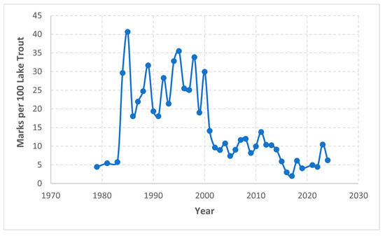
Figure 1.
Sea lamprey (Petromyzon marinus) wounding rates on adult (>533 mm) lake trout (Salvelinus namaycush) from the annual spring gillnetting surveys conducted by the Michigan Department of Natural Resources in US waters of Lake Huron.
The Michigan Department of Natural Resources (MIDNR) has maintained the annual spring gillnet survey in US waters of Lake Huron since 1970 [24,25,48]. This fishery-independent survey uses multi-mesh multifilament gillnets set in nearshore waters (10–60 m depth) and is typically conducted from late April through early June before lake stratification. The gillnets include nine single-mesh panels, each 30.5 m long and 1.83 m tall, with stretch mesh sizes of 50.8 to 152.4 mm in 12.7 mm increments. Lake trout were caught with gillnets set overnight on the lake bottom. All hatchery-stocked lake trout were identified based on the presence of a fin clip, and lake trout without a fin clip were considered wild. Age assignments were based on coded-wire tag information, fin clips, or a combination of fin clip and maxilla sections for hatchery-stocked fish, and maxilla or otolith sections for wild fish [50,51]. All individual fish samples were summarized by year, age, and recruitment origin (stocked or wild). Within a sampling year (Yr), the year-class (Yc) for each age group was calculated as Yc = Yr − Age. The first year that lake trout were caught in the annual spring gillnet survey was 1975, and, therefore, our analyses included data for the years 1975–2024.
2.2. Model Comparison and Selection
The age, year, and year-class effects could be structured in more than one model, and therefore, model comparison and selection procedures based on the Akaike information criterion (AIC) [52] and the Bayesian information criterion (BIC) [53] were used to arrive at the best model for estimating YCS. The best model was not expected to be the same between AIC and BIC comparisons [54,55]. YCS estimates were expected to be similar between the best model based on AIC and the best model based on BIC.
The age at which lake trout first fully recruited to the fishing gears was not constant across years in the main basin of Lake Huron but was within a narrow age range of 5–7 years [20]. Longitudinal analysis was implemented using this age range, and 14 model structures were compared:
here, represents the catch (number of fish) at each age, ε is the residual error of the model prediction, and the mean of the residual errors is equal to zero. The data do not have to be expressed in the form of age-specific catch per unit of effort (CPUE), because the model has included a year effect that represents interannual variations in fishing or sampling effort and catchability. All equations herein use Greek letters (e.g., α, β, and γ) to represent fixed effects, and Roman letters (e.g., ) to represent random effects [56]. The subscript Age stands for fish age, Yr stands for sampling year, and Yc stands for year-class. HW stands for recruitment origin (hatchery or wild), and thus (Age.HW), (Yr.HW), and (Yc.HW) represent the interactions between recruitment origin with fish age, sampling year, and year-class, respectively. For all models in this paper, the age effect was used to incorporate an exponential decline in year-class abundance through time, which could be mediated by age-specific selectivity and mortality. Log-transformation of the data was appropriate for modeling this population process [20,23,24,25,26].
Equations (1)–(9) had one of the three major factors (the age, year-class, and sampling year) as a fixed effect, either entering or not entering an interaction with recruitment origin, and the other two major factors as random effects. Equations (1)–(3) had year-class as the fixed effect, as YCS had the primary impact on the catch of a fish year-class across ages and years. The age and year effects were modeled as random effects, reflecting the reality that the same age range was selected for multiple measures on every year-class, while a different year range was used for each year-class.
Equations (4)–(6) had fish age as a fixed effect, and year-class and year as random effects. These models emphasized age-specific selectivity and mortality to reveal the process by which year-class abundance diminishes through time, along with random variations in year-class strength, year-specific fishing or sampling effort, and catchability. Note that Equations (1)–(3) vs. Equations (4)–(6) represented alternative understandings of the three major factors affecting catch-at-age data, but these alternative views were not necessarily in conflict.
Equations (7)–(9) had sampling year as the fixed effect. Year-class and fish age were included as random effects. Such alternative depictions of major factors affecting catch-at-age data appeared to be in contrast to the above understanding of the year-class or age effect as the fixed effect, but were objectively evaluated through model comparisons based on AIC and BIC.
Equations (10)–(14) had both year-class and age as fixed effects. Several other model structures with two of the three major factors as fixed effects were also evaluated in preliminary analyses, such as Equations (15) and (16) below.
these models failed to converge and are, therefore, not reported in the Results. In contrast to a previous study [20], recruitment origin was also included as a factor in the current study, in addition to the three major factors of age, year, and year-class. This additional factor reflected the reality and complexity embodied in the data, but not every year had number-at-age observations for both stocked and wild lake trout. Also, in general, it is not statistically possible to have the age, year (Yr), and year-class (Yc) all as fixed effects because at least one level of these major factors cannot be independently estimated given the relationship of Yr = Age + Yc.
The following three linear mixed-effects models were evaluated for catch-curve regression, building on the results from previous studies that have found no difference in adult mortality between stocked and wild lake trout [24,25]:
here, unlike Equations (1)–(16), Age is used as a numerical variable rather than a categorical variable. α is the intercept of the regression line, β is the regression slope representing the instantaneous total mortality, ε stands for the residual error, and the mean residual error is equal to zero. In Equation (17), α is the average intercept. In Equations (18) and (19), the average intercept is dropped, and the fixed effects stand for cohort-specific or year-specific intercepts. To exert an effect on the intercept, both year-class and year enter an interaction with recruitment origin (hatchery or wild; HW). The first model (Equation (17)) had both year-class (Yc) and sampling year (Yr) as random effects on the intercept. The second model (Equation (18)) had year-class as a fixed effect and year as a random effect. The third model (Equation (19)) had year as a fixed effect and year-class as a random effect. Again, is the catch-at-age number of fish. The analysis was applied to the data expressed as number of fish rather than CPUE, because variation in year-specific sampling efforts and in year-specific catchability were incorporated in year effects on the intercept.
In conventional year-specific catch-curve regression, the residuals from model predictions are associated with variation in year-class strength, and in conventional cohort-specific catch-curve regression, the intercept represents year-class strength [57,58,59]. Equations (17)–(19) have integrated those basic properties into the linear mixed-effects models for catch-curve regression to estimate both year-class and year effects on the intercept. Also note that statistical concerns with the conventional catch-curve regression and various recommendations for the best practices mostly arise from the use of year-specific or cohort-specific data [60,61,62,63,64,65]. By using data for multiple observations on every year-class and from every sampling year, Equations (17)–(19) have time-dependent YCS and catchability incorporated in the regression models for estimating adult mortality during a given time period.
Equations (17)–(19) were implemented with data for each of the two time periods identified in earlier studies, i.e., pre- and post-2000 [24,25]. See also Figure 1. The effective age range was 5–11 years for the first time period of 1975–1999, and 7–15 years for the second time period of 2000–2024, based on average number-at-age [24,25]. Prior to 2000, the abundance and survey catch of wild lake trout were negligible, and the analyses focused only on stocked lake trout; as such, recruitment origin (HW) was dropped from the equations. All linear-mixed models in our analyses were implemented using the base package of “nlme” in R with the maximum likelihood option [66,67].
3. Results
For longitudinal analysis of the full time-series of 1975–2024, the best model based on AIC was Equation (2), which had year-class interacting with recruitment origin as a fixed effect, sampling year as a random effect, and fish age interacting with recruitment origin as another random effect (Table 1). Based on BIC, however, the best model was Equation (5), which had fish age interacting with recruitment origin as a fixed effect, sampling year as a random effect, and year-class interacting with recruitment origin also as a random effect. Log-likelihood values indicated that the best model based on AIC provided much better data fits than the best model based on BIC. Having both year-class and age as fixed effects and year-class interacting with recruitment origin in Equation (12) provided the best data fits, but that model was not supported by either AIC or BIC comparison. YCS patterns and trends estimated as a fixed effect from the best model based on AIC were consistent with those estimated as a random effect from the best model based on BIC (Equation (5) vs. Equation (2); Figure 2).

Table 1.
Model comparison and selection based on the Akaike information criterion (AIC) and Bayesian information criterion (BIC) for reconstructing lake trout (Salvelinus namaycush) year-class strength in US waters of Lake Huron using catch-at-age data collected during 1975–2024 and linear mixed-effects models for longitudinal analyses. Model structures include three major factors of the age, year-class (Yc), and sampling year (Yr), with or without interaction with recruitment origin, such as hatchery-stocked and wild lake trout (HW). The factors in parentheses indicate random effects. Provided is the degree of freedom (df) of each model, and the difference in AIC (ΔAIC) and BIC (ΔBIC) between a model and the best model, with the best model having ΔAIC = 0 or ΔBIC = 0 (with bold font). Negative log-likelihood values are also provided to compare data fits.
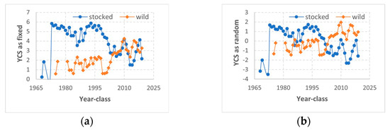
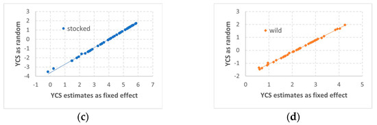
Figure 2.
Lake trout (Salvelinus namaycush) year-class strength (YCS) reconstructed from linear mixed-effects models for longitudinal analysis, based on numbers of fish at ages 5–7 from the annual spring gillnetting surveys (1975–2024) conducted by Michigan Department of Natural Resources in US waters of Lake Huron. (a) Lake trout YCS estimated with year-class as a fixed effect from the best model based on Akaike information criterion (AIC). (b) Lake trout YCS estimated with year-class as a random effect from the best model based on Bayesian information criterion (BIC). (c) YCS for stocked lake trout estimated with year-class as a random effect (based on BIC) plotted against the estimates with year-class as a fixed effect (based on AIC). (d) YCS for wild lake trout estimated with year-class as a random effect (based on BIC) plotted against the estimates with year-class as a fixed effect (based on AIC).
For catch-curve regression using linear mixed-effects models, the best models were not the same for the two different time periods. Based on data collected prior to 2000 for hatchery-stocked lake trout, the best model was supported by both AIC and BIC comparisons, and the model had year as a fixed effect on the intercept and year-class as a random effect on the intercept (Equation (19); Table 2). During 2000–2024, data complexity increased and included both stocked and wild lake trout. For this time period, the best model for catch-curve regression was not the same from AIC and BIC comparisons (Table 3). Based on AIC, the best model had year-class interacting with recruitment origin as a fixed effect on the intercept, and sampling year interacting with recruitment origin as a random effect on the intercept (Equation (18)). Based on BIC, the best model had year-class interacting with recruitment origin, and sampling year interacting with recruitment origin, both as random effects on the intercept (Equation (17)). YCS patterns and trends estimated with year-class as a fixed effect from the best model based on AIC were consistent with those estimated with year-class as a random effect from the best model based on BIC (Equation (18) vs. Equation (17); Figure 3). In closer comparison, the random effect estimates showed slightly greater variance for lower YCS estimates (Figure 3).
Table 2.
Model comparisons and selection based on the Akaike information criterion (AIC) and Bayesian information criterion (BIC) for reconstructing year-class strength of hatchery-stocked lake trout (Salvelinus namaycush) in US waters of Lake Huron using catch-at-age data collected during 1975–1999 and linear mixed-effect models for catch-curve regression. Model structures include the Age as a numerical variable, and year-class (Yc) and sampling year (Yr) as factors. The factors in parentheses indicate random effects. Provided is the degree of freedom (df) of each model, and the difference in AIC (ΔAIC) and BIC (ΔBIC) between a model and the best model, with the best model having ΔAIC = 0 and ΔBIC = 0 (with bold font). Negative log-likelihood values are also provided to compare data fits.
Table 3.
Model comparisons and selection based on the Akaike information criterion (AIC) and Bayesian information criterion (BIC), for reconstructing year-class strength of lake trout (Salvelinus namaycush) in US waters of Lake Huron using catch-at-age data collected during 2000–2024 and linear mixed-effects models for catch-curve regression. Model structures include age as a numerical variable and year-class (Yc) and sampling year (Yr) as factors with interaction to recruitment origin, such as hatchery-stocked and wild lake trout (HW). The factors in parentheses indicate random effects. Provided is the degree of freedom (df) of each model, and the difference in AIC (ΔAIC) and BIC (ΔBIC) between a model and the best model, with the best model having ΔAIC = 0 or ΔBIC = 0 (with bold font). Negative log-likelihood values are also provided to compare data fits.
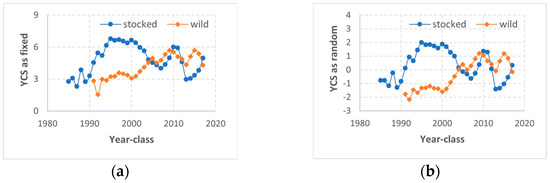
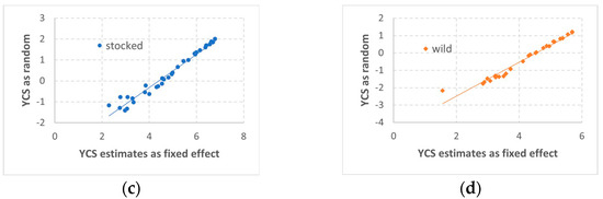
Figure 3.
Lake trout (Salvelinus namaycush) year-class strength (YCS) reconstructed from linear mixed-effect models for catch-curve regression, based on catch-at-age data from the annual spring gillnetting surveys (2000–2024) conducted by the Michigan Department of Natural Resources in US waters of Lake Huron. (a) Lake trout YCS estimated with year-class as a fixed effect from the best model based on Akaike information criterion (AIC). (b) Lake trout YCS estimated with year-class as a random effect from the best model based on the Bayesian information criterion (BIC). (c) YCS for stocked lake trout estimated with year-class as a random effect (based on BIC) plotted against the estimates with year-class as a fixed effect (based on AIC). (d) YCS for wild lake trout estimated with year-class as a random effect (based on BIC) plotted against the estimates with year-class as a fixed effect (based on AIC).
Using data collected prior to 2000, the linear mixed-effects model for catch-curve regression estimated YCS for the 1968–1994 year-classes of hatchery-stocked lake trout. The estimated YCS patterns and trends were consistent with those estimated from the linear mixed-effects model for longitudinal analysis, with a few exceptions, including the four earliest year-classes (Figure 4a,b).
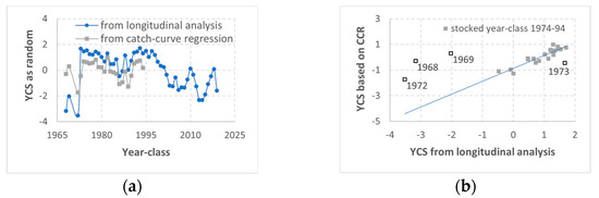
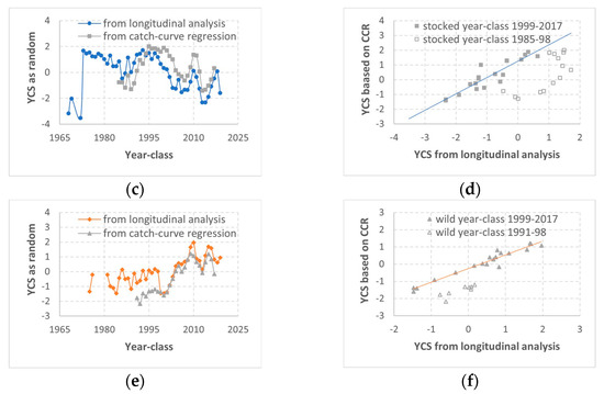
Figure 4.
Estimates of lake trout (Salvelinus namaycush) year-class strength (YCS) were compared between the linear mixed-effect models for longitudinal analysis of catch-at-age data and for catch-curve regression, based on the annual spring gillnetting surveys conducted by the Michigan Department of Natural Resources in US waters of Lake Huron. (a,b) YCS for stocked lake trout as estimated with year-class as a random effect from the catch-curve regression (CCR) using 1975–1999 data, compared to the estimates with year-class as a random effect from the longitudinal analysis of 1975–2024 data. (c,d) YCS for stocked lake trout as estimated with year-class as a random effect from the catch-curve regression (CCR) using 2000–2024 data, compared to the estimates with year-class as a random effect from the longitudinal analysis of 1975–2024 data. (e,f) YCS for wild lake trout as estimated with year-class as a random effect from the catch-curve regression (CCR) using 2000–2024 data, compared to the estimates with year-class as a random effect from the longitudinal analysis of 1975–2024 data.
Using data collected during 2000–2024, the linear mixed-effects model for catch-curve regression estimated YCS for the 1985–2017 year-classes of hatchery-stocked lake trout and the 1991–2017 year-classes of wild lake trout. For the 1999 and more recent year-classes, and for both stocked and wild lake trout, the estimated YCS patterns and trends were consistent with the estimates from the longitudinal analyses (Figure 4c–f). For the 1985–1998 year-classes, however, and for both stocked and wild lake trout, the catch-curve estimates of YCS were substantially lower than those estimates from the longitudinal analysis.
4. Discussion
With applications to the same time series of catch-at-age data, the linear mixed-effects models for longitudinal analysis and for catch-curve regression reconstructed the same or similar YCS patterns and trends for lake trout in the main basin of Lake Huron. These results suggest that each of these two modeling approaches provides a robust statistical framework for estimating YCS in fish populations. To further demonstrate the general applicability of these two modeling approaches, future studies may investigate other fish populations to determine whether or not the YCS patterns and trends generated from these two modeling approaches are in good agreement with one another, just as we found from our application to the Lake Huron lake trout population.
Our results have direct implications for practical fishery management. First, it is often difficult to maintain specialized survey efforts for indexing fish recruitment at a given young age, and our findings have demonstrated a complementary approach that annual collection of biological data can be fully explored for reliable YCS estimates. Second, by using the same standard and relatively simple methods, the estimates of fish population metrics will be comparable between independent time series of data collection. All linear mixed-effects models in this paper were implemented using the base package of “nlme” in R [66,67], and more advanced statistical packages are not reviewed in this paper. We emphasized applications of the basic statistical principles for analyzing time series of catch-at-age data. This is essential for improving the collection and analysis of fish population data that are always influenced by fish age, year-class, and sampling year.
For lake trout in the main basin of Lake Huron, the estimated YCS patterns and trends reflected the chronology of the annual stocking of hatchery-reared juvenile lake trout and recent increases in recruitment of wild lake trout. The rapid increase in year-class strength during the early 1970s was consistent with coordinated stocking efforts [68]. The decrease in YCS during the mid-1980s could be explained by the relatively low alewife abundance during these years [69]. As the protective buffer of alewife abundance thinned, the predation on newly stocked juvenile lake trout perhaps increased. During the late 1980s and early 1990s, the increase in YCS was likely due to improved stocking efforts [39], including (1) stocking on offshore reefs, (2) offshore vessel stocking, (3) increases in the stocked proportion of deep-water lake trout strains such as the Seneca Lake strain, (4) increases in the size and body condition of juvenile lake trout at stocking, and (5) increases in the annual stocking rates. During the late 1980s and early 1990s, alewife abundance also temporarily recovered [69]. Since the end of the 1990s and the beginning of the 2000s, the dramatic decline in YCS of hatchery-stocked lake trout and the increase in YCS of wild lake trout reflected regime shifts within the ecosystem and in lake trout recruitment that are characterized by the collapse of alewives and the observation that lake wide increases in recruitment of wild lake trout did not fully compensate for the dramatic declines in survival and recruitment of hatchery-stocked lake trout [11,12,46,47,48,49].
For some early-year classes, some differences in YCS estimates were detected between the linear mixed-effects models for catch-curve regression and for longitudinal analysis of catch-at-age data. Those differences were likely to be due to abrupt changes in adult lake trout mortality over time that influenced YCS estimates from the catch-curve regressions. For example, the 1968, 1969, and 1972 YCS from catch-curve regression were likely overestimated because those year-classes experienced much lower fishing and total mortality than the 1974–1994 year-classes. Likewise, the 1973 YCS was likely underestimated because the 1973 year-class experienced much higher fishing and total mortality than the year-classes produced during 1974–1994. The contrast between 1973 and the other three earlier year-classes reflected the process that continued stocking generated commercial and recreational fisheries, and thereafter, regulations were imposed on commercial and recreational harvests. Also related to rapid changes in adult mortality, lake trout of the 1985–1998 year-classes lived through two time periods. Based on the results of catch-curve regression, instantaneous total mortality for adult lake trout was 0.63 prior to 2000, but only 0.24 during 2000–2024, and these mortality estimates were consistent with those from previous studies [23,24,25]. From 2000–2024 data, the catch-curve regressions estimated YCS (year-class specific intercepts) based on the current mortality rate (the regression slope) that was much lower than the mortality experienced by the 1985–1998 year-classes prior to 2000, and thus, YCS for those earlier year-classes were underestimated in comparison to the estimates from the longitudinal analysis of the same data. Thus, year-class effects from the longitudinal analysis are more robustly separated from the age and year effects, and YCS estimates are robust to long-term ecosystem changes, such as those that have occurred in Lake Huron [70,71,72,73].
For longitudinal analysis of catch-at-age data, the best model structure based on either AIC or BIC in this study was not the same as in the previous study using the same approach [20]. In fact, the model structure similar to the best model in the previous study failed to converge in this current study (Equation (16)). The difference between the current and previous study likely stemmed from the data complexity being analyzed or ignored. The current study addressed the embodied complexity of more than one recruitment origin (hatchery-stocked and wild lake trout). In the previous study, multiple data sources were indexed and combined, and in that context, the embodied complexity of recruitment origin was ignored.
Model comparison and selection based on information criteria has also added both insight and complexity to the analyses. It is well accepted to determine model structure in ecological studies through objective model comparisons, but it is still a practical challenge when the best model based on AIC and BIC is not necessarily the same [54,55]. From our methods, the random effects are not added to the description of a particular process. Rather, the linear mixed-effects models are used to separate three major processes that are embodied in catch-at-age data. In that regard, the model development decision is about a major factor to be included as a fixed or random effect in the model, and the decision cannot be fully dependent on prior knowledge, such as the primary interest of an investigation and whether or not a variable has systematic patterns and trends. From our findings, the best model may or may not be the same based on AIC or BIC (Table 1, Table 2 and Table 3). When the best model is not the same based on AIC or BIC (Table 1 and Table 3), we found that YCS patterns and trends estimated with year-class as a fixed effect based on AIC are consistent with those estimated with year-class as a random effect based on BIC. The implication is that, after objective model comparison and selection, the best model based on AIC or BIC may have emphasized different aspects of the data that are not necessarily in conflict.
5. Conclusions
We found that in our application to the lake trout population in Lake Huron, via objective model comparison and selection, the estimated YCS patterns and trends were the same or similar between the two substantially different modeling approaches applied to the same time series of catch-at-age data. Recent studies have applied the linear mixed-effects models for longitudinal analysis of catch-at-age data to four fish species [18,19,20,21,22], including walleye (Sander vitreus), lake trout, lake whitefish (Coregonus clupeaformis), and alewives. The linear mixed-effects models for catch-curve regression have been applied to two fish species [23,24,25,26], including lake trout and lake whitefish. A comparison of YCS estimates from both approaches, however, has yet to be undertaken for walleye, lake whitefish, or alewives. In future studies, with care for potential caveats as we explicitly discussed, both modeling approaches could be applied to analyze time series of catch-at-age data for fish populations other than lake trout populations to determine if such applications yield similar results as ours, namely that both approaches generate the same or similar patterns and trends in YCS estimates for a given fish population. The needed model development may first explore and address the embodied complexities within each time series of catch-at-age data, before integrated analyses being conducted using multiple data sources, such as to integrate findings from every data source by calculating the weighted average YCS [5,20,26].
Author Contributions
Conceptualization: J.X.H. and C.P.M.; methodology: J.X.H.; validation: C.P.M.; formal analysis: J.X.H. and C.P.M.; investigation: J.X.H. and C.P.M.; data curation: J.X.H.; writing—original draft preparation: J.X.H.; writing—review and editing: C.P.M.; visualization: J.X.H. All authors have read and agreed to the published version of the manuscript.
Funding
This research received no external funding.
Institutional Review Board Statement
Not applicable.
Informed Consent Statement
Not applicable.
Data Availability Statement
All data analyzed and generated by this study are available upon a reasonable request to the corresponding author.
Acknowledgments
This study was funded with financial support from the Federal Aid in Sport Fish Restoration Program F-61 to the Michigan Department of Natural Resources, Fishery Division, Studies 230451 and 230522, at Lake Huron Research Station. Any use of trade, firm, or product names is for descriptive purposes only and does not imply endorsement by the U.S. Government.
Conflicts of Interest
The authors declare no conflicts of interest.
Abbreviations
The following abbreviations are used in this manuscript:
| YCS | Year-class strength |
| AIC | Akaike information criterion |
| BIC | Bayesian information criterion |
| CCR | Catch curve regression |
| CPUE | Catch per unit of effort. |
References
- Shepherd, J.G.; Cushing, D.H. Regulation in fish populations: Myth or mirage? Phil. Trans. R. Soc. Lond. B 1990, 330, 151–164. [Google Scholar]
- Rothschild, B.J. “Fish stocks and recruitment”: The past thirty years. ICES J. Mar. Sci. 2000, 57, 191–201. [Google Scholar] [CrossRef]
- Subbey, S.; Devine, J.A.; Schaarschmidt, U.; Nash, R.D.M. Modelling and forecasting stock–recruitment: Current and future perspectives. ICES J. Mar. Sci. 2014, 71, 2307–2322. [Google Scholar] [CrossRef]
- Rosenberg, A.A.; Kirkwood, G.P.; Cook, R.M.; Myers, R.A. Combining information from commercial catches and research surveys to estimate recruitment: A comparison of methods. ICES J. Mar. Sci. 1992, 49, 379–387. [Google Scholar] [CrossRef]
- Shepherd, J.G. Prediction of year-class strength by calibration regression analysis of multiple recruit index series. ICES J. Mar. Sci. 1997, 54, 741–752. [Google Scholar] [CrossRef]
- Rose, G.A.; Kulka, D.W. Hyper aggregation of fish and fisheries: How catch-per-unit-effort increased as the northern cod (Gadus morhua) declined. Can. J. Fish. Aquat. Sci. 1999, 56, 118–127. [Google Scholar] [CrossRef]
- Harley, S.J.; Myers, R.A.; Dunn, A. Is catch-per-unit-effort proportional to abundance? Can. J. Fish. Aquat. Sci. 2001, 58, 1760–1772. [Google Scholar] [CrossRef]
- Wilberg, M.J.; Bence, J.R. Performance of time-varying catchability estimators in statistical catch-at-age analysis. Can. J. Fish. Aquat. Sci. 2006, 63, 2275–2285. [Google Scholar] [CrossRef]
- He, J.X.; Stewart, D.J. Age and size at first reproduction of fishes: Predictive models based only on growth trajectories. Ecology 2001, 82, 784–791. [Google Scholar] [CrossRef]
- He, J.X.; Stewart, D.J. A stage-explicit expression of the von Bertalanffy growth model for understanding age at first reproduction of Great Lakes fishes. Can. J. Fish. Aquat. Sci. 2002, 59, 250–261. [Google Scholar] [CrossRef]
- He, J.X.; Bence, J.R.; Madenjian, C.P.; Pothoven, S.A.; Dobiesz, N.E.; Fielder, D.G.; Johnson, J.E.; Ebener, M.P.; Cottrill, A.R.; Mohr, L.C.; et al. Coupling age-structured stock assessment and fish bioenergetics models: A system of time-varying models for quantifying piscivory patterns during the rapid trophic shift in the main basin of Lake Huron. Can. J. Fish. Aquat. Sci. 2015, 72, 7–23. [Google Scholar] [CrossRef]
- He, J.X.; Bence, J.R.; Madenjian, C.P.; Claramunt, R. Dynamics of lake trout production in the main basin of Lake Huron. ICES J. Mar. Sci. 2020, 73, 975–987. [Google Scholar] [CrossRef]
- Smith, P.E. Year-class strength and survival of 0-group Clupeoids. Can. J. Fish. Aquat. Sci. 1985, 42, 69–82. [Google Scholar] [CrossRef]
- Thanassekos, S.; Latour, R.J.; Fabrizio, M.C. An individual-based approach to year-class strength estimation. ICES J. Mar. Sci. 2016, 73, 2252–2266. [Google Scholar] [CrossRef]
- Myers, R.A. Recruitment: Understanding density-dependence in fish populations. In Handbook of Fish Biology and Fisheries; Hart, P.J.B., Reynolds, J.D., Eds.; Blackwell Publishing: Oxford, UK, 2002; Volume 1, pp. 123–148. [Google Scholar]
- Maceina, M.J.; Pereira, D.L. Recruitment. In Analysis and Interpretation of Freshwater Fisheries Data; Guy, C., Brown, M.L., Eds.; American Fisheries Society: Bethesda, MD, USA, 2007; pp. 121–185. [Google Scholar]
- Carlander, K.D.; Payne, P.M. Year-class abundance, population, and production of walleye (Stizostedion vitreum vitreum) in Clear Lake, Iowa, 1948–1974, with varied fry stocking rates. J. Fish. Res. Board Can. 1977, 34, 1792–1799. [Google Scholar] [CrossRef]
- Parsons, B.G.; Pereira, D.L. Relationship between walleye stocking and year-class strength in three Minnesota lakes. N. Am. J. Fish. Manag. 2001, 21, 801–808. [Google Scholar] [CrossRef]
- Honsey, A.E.; Zachary, S.; Feiner, Z.S.; Hansen, G.J.A. Drivers of walleye recruitment in Minnesota’s large lakes. Can. J. Fish. Aquat. Sci. 2020, 77, 1921–1933. [Google Scholar] [CrossRef]
- He, J.X.; Honsey, A.E.; Staples, D.F.; Bence, J.R.; Claramunt, T. Longitudinal analyses of catch-at-age data for reconstructing year-class strength, with an application to lake trout (Salvelinus namaycush) in the main basin of Lake Huron. Can. J. Fish. Aquat. Sci. 2023, 80, 183–194. [Google Scholar] [CrossRef]
- Warren, L.D.; Honsey, A.E.; Bunnell, D.B.; Collingsworth, P.D.; Hondorp, D.W.; Madenjian, C.P.; Warner, D.M.; Weidel, B.C.; Höök, T.O. Synchrony of alewife, Alosa pseudoharengus, year-class strength in the Great Lakes region. Can. J. Fish. Aquat. Sci. 2025, 81, 1456–1467. [Google Scholar] [CrossRef]
- Brown, T.A.; Rudstam, L.G.; Sethi, S.A.; Ripple, P.; Smith, J.B.; Treska, T.J.; Hessell, C.; Olsen, E.; He, J.X.; Jonas, J.L.; et al. Reconstructing half a century of coregonine recruitment dynamics across the Laurentian Great Lakes. ICES J. Mar. Sci. 2025, 82, fsae160. [Google Scholar] [CrossRef]
- He, J.X.; Ebener, M.P.; Clark, R.D., Jr.; Bence, J.R.; Madenjian, C.P.; McDonnell, K.N.; Bronte, C.R. Estimating catch curve mortality based on relative return rates of coded wire tagged lake trout in U.S. waters of Lake Huron. Can. J. Fish. Aquat. Sci. 2022, 79, 601–610. [Google Scholar] [CrossRef]
- He, J.X.; Madenjian, C.P.; Wills, T.C. A generalized application of the catch-curve regression with comparisons of adult mortality and year-class strength between hatchery-stocked and wild-reared lake trout in US waters of Lake Huron. Can. J. Fish. Aquat. Sci. 2023, 80, 1714–1722. [Google Scholar] [CrossRef]
- He, J.X. Adult mortality and year-class strength of lake trout before and after alewife collapse in the main basin of Lake Huron. J. Great Lakes Res. 2024, 50, 102397. [Google Scholar] [CrossRef]
- He, J.X.; Briggs, A.S.; Wills, T.C. Year-class strength and fully-selected mortality rates of Lake Whitefish in Michigan waters of southern Lake Huron. N. Am. J. Fish. Manag. 2024. [Google Scholar] [CrossRef]
- Maunder, M.N.; Punt, A.E. A review of integrated analysis in fisheries stock assessment. Fish. Res. 2013, 142, 61–74. [Google Scholar] [CrossRef]
- Methot, R.D., Jr.; Wetzel, C.R. Stock synthesis: A biological and statistical framework for fish stock assessment and fishery management. Fish. Res. 2013, 142, 86–99. [Google Scholar] [CrossRef]
- Nielsen, A.; Berg, C.W. Estimation of time-varying selectivity in stock assessments using state-space models. Fish. Res. 2014, 158, 96–101. [Google Scholar] [CrossRef]
- Aeberhard, W.H.; Flemming, J.M.; Nielsen, A. Review of state-space models for fisheries science. Annu. Rev. Stat. Appl. 2018, 5, 215–235. [Google Scholar] [CrossRef]
- Cheng, M.L.H.; Thorson, J.T.; Ianelli, J.N.; Cunningham, C.J. Unlocking the triad of age, year, and cohort effects for stock assessment: Demonstration of a computationally efficient and reproducible framework using weight-at-age. Fish. Res. 2023, 266, 106755. [Google Scholar] [CrossRef]
- Mohn, R. The retrospective problem in sequential population analysis: An investigation using cod fishery and simulated data. ICES J. Mar. Sci. 1999, 56, 473–488. [Google Scholar] [CrossRef]
- Hile, R. Trends in the lake trout fishery of Lake Huron through 1946. Trans. Am. Fish. Soc. 1949, 76, 121–147. [Google Scholar] [CrossRef]
- Walters, C.J.; Steer, G.; Spangler, G. Responses of lake trout (Salvelinus namaycush) to harvesting, stocking, and lamprey reduction. Can. J. Fish. Aquat. Sci. 1980, 37, 2133–2145. [Google Scholar] [CrossRef]
- Smith, S.H. Species succession and fishery exploitation in the Great Lakes. J. Fish. Res. Board Can. 1968, 25, 667–693. [Google Scholar] [CrossRef]
- Muir, A.M.; Krueger, C.C.; Hansen, M.J. Re-establishing lake trout in the Laurentian Great Lakes: Past, present, and future. In Great Lakes Fisheries Policy and Management: A Binational Perspective, 2nd ed.; Taylor, W.W., Lynch, A.J., Leonard, N.J., Eds.; Michigan State University Press: East Lansing, MI, USA, 2012; pp. 533–588. [Google Scholar]
- He, J.X. Growth stability after the collapse of alewives in Lake Huron and direct size-at-age comparisons between stocked and wild lake trout. J. Great Lakes Res. 2024, 50, 102315. [Google Scholar] [CrossRef]
- Sitar, S.P.; Bence, J.R.; Johnson, J.E.; Ebener, M.P.; Taylor, W.W. Lake trout mortality and abundance in southern Lake Huron. N. Am. J. Fish. Manag. 1999, 19, 881–900. [Google Scholar] [CrossRef]
- Johnson, J.E.; He, J.X.; Woldt, A.P.; Ebener, M.P.; Mohr, L.C. Lessons in rehabilitation stocking and management of lake trout in Lake Huron. Am. Fish. Soc. Symp. 2004, 44, 161–175. [Google Scholar]
- Walters, C.; Kitchell, J.F. Cultivation/depensation effects on juvenile survival and recruitment: Implications for the theory of fishing. Can. J. Fish. Aquat. Sci. 2001, 58, 39–50. [Google Scholar] [CrossRef]
- Madenjian, C.P.; O’Gorman, R.; Bunnell, D.B.; Argyle, R.L.; Roseman, E.F.; Warner, D.M.; Stockwell, J.D.; Stapanian, M.A. Adverse effects of alewives on Laurentian Great Lakes fish communities. N. Am. J. Fish. Manag. 2008, 28, 263–282. [Google Scholar] [CrossRef]
- Fitzsimons, J.D.; Brown, S.; Brown, L.; Honeyfield, D.; He, J.; Johnson, J.E. 2010. Increase in lake trout reproduction in Lake Huron following the collapse of alewife: Relief from thiamine deficiency or larval predation? Aquat. Ecosyst. Health Manag. 2010, 13, 73–81. [Google Scholar] [CrossRef]
- Adams, J.V.; Bergstedt, R.A.; Christie, G.C.; Cuddy, D.W.; Fodale, M.F.; Heinrich, J.W.; Jones, M.L.; McDonald, R.B.; Mullett, K.M.; Young, R.J. Assessing assessment: Can the expected effects of the St. Marys River sea lamprey control strategy be detected? J. Great Lakes Res. 2003, 29, 717–727. [Google Scholar] [CrossRef]
- Nowicki, S.M.; Criger, L.A.; Hrodey, P.J.; Sullivan, W.P.; Neave, F.B.; He, J.X.; Gorenflo, T.K. A case history of sea lamprey (Petromyzon marinus) abundance and control in Lake Huron: 2000–2019. J. Great Lakes Res. 2021, 47, 455–478. [Google Scholar] [CrossRef]
- United States v. Michigan. Consent Decree. 2000; Case No. 2:73 CV 26. [Google Scholar]
- Riley, S.C.; Roseman, E.F.; Nichols, S.J.; O’Brien, T.P.; Kiley, C.S.; Schaeffer, J.S. Deepwater demersal fish community collapse in Lake Huron. Trans. Am. Fish. Soc. 2008, 137, 1879–1890. [Google Scholar] [CrossRef]
- Riley, S.C.; He, J.X.; Johnson, J.E.; O’Brien, T.P.; Schaeffer, J.S. Evidence of widespread natural reproduction by lake trout Salvelinus namaycush in the Michigan Waters of Lake Huron. J. Great Lakes Res. 2007, 33, 917–921. [Google Scholar] [CrossRef]
- He, J.X.; Ebener, M.P.; Riley, S.C.; Cottrill, A.; Kowalski, A.; Koproski, S.; Mohr, L.; Johnson, J.E. Lake Trout Status in the Main Basin of Lake Huron, 1973–2010. N. Am. J. Fish. Manag. 2012, 32, 402–412. [Google Scholar] [CrossRef]
- Johnson, J.E.; He, J.X.; Fielder, D.G. Rehabilitation stocking of walleyes and lake trout: Restoration of reproducing stocks in Michigan waters of Lake Huron. N. Am. J. Fish. Aquac. 2015, 77, 396–408. [Google Scholar] [CrossRef]
- Wellenkamp, W.; He, J.X.; Vercnocke, D. Using Maxillae to Estimate Ages of Lake Trout. N. Am. J. Fish. Manag. 2015, 35, 296–301. [Google Scholar] [CrossRef]
- Murphy, E.W.; Smith, M.L.; He, J.X.; Wellenkamp, W.; Barr, E.; Downey, P.C.; Miller, K.M.; Meyer, K.A. Revised fish aging techniques improve fish contaminant trend analyses in the face of changing Great Lakes food webs. J. Great Lakes Res. 2018, 44, 725–734. [Google Scholar] [CrossRef]
- Akaike, H. Information theory and an extension of the maximum likelihood principle. In Proceedings of the Second International Symposium on Information Theory; Petrov, B.N., Csáki, F., Eds.; Akadémiai Kiadó: Budapest, Hungary, 1973; pp. 267–281. [Google Scholar]
- Schwarz, G. 1978. Estimating the dimension of a model. Ann. Stat. 1978, 6, 461–464. [Google Scholar] [CrossRef]
- Burnham, K.P.; Anderson, D.R. Model Selection and Multi-Model Inference: A Practical Information-Theoretic Approach, 2nd ed.; Springer: New York, NY, USA, 2002. [Google Scholar]
- Aho, K.; Derryberry, D.; Peterson, T. Model selection for ecologists: The worldviews of AIC and BIC. Ecology 2014, 95, 631–636. [Google Scholar] [CrossRef]
- McCulloch, C.M.; Searle, S.R.; Neuhaus, J.M. Generalized, linear, and mixed Models, 2nd ed.; John Wiley & Sons: Hoboken, NJ, USA, 2008. [Google Scholar]
- Hilborn, R.; Walters, C.J. Quantitative Fisheries Stock Assessment, Choice, Dynamics and Uncertainty; Chapman and Hall: New York, NY, USA, 1992. [Google Scholar]
- Maceina, M.J. Simple application of using residuals from catch-curve regressions to assess year-class strength in fish. Fish. Res. 1997, 32, 115–121. [Google Scholar] [CrossRef]
- Tetzlaff, J.C.; Catalano, M.J.; Allen, M.S.; Pine, W.E. Evaluation of two methods for indexing fish year-class strength: Catch-curve residuals and cohort method. Fish. Res. 2011, 109, 303–310. [Google Scholar] [CrossRef]
- Ricker, W.E. Computation and interpretation of biological statistics of fish populations. Bull. Fish. Res. Board Can. 1975, 191, 382. [Google Scholar]
- Dunn, A.; Francis, R.I.C.C.; Doonan, I.J. Comparison of the Chapman–Robson and regression estimators of Z from catch-curve data when non-sampling stochastic error is present. Fish. Res. 2002, 59, 149–159. [Google Scholar] [CrossRef]
- Smith, M.W.; Then, A.Y.; Wor, C.; Ralph, G.; Pollock, K.H.; Hoenig, J.M. Recommendations for catch-curve analysis. N. Am. J. Fish. Manag. 2012, 32, 956–967. [Google Scholar] [CrossRef]
- Millar, R.B. A better estimator of mortality rate from age frequency data. Can. J. Fish. Aquat. Sci. 2015, 72, 364–375. [Google Scholar] [CrossRef]
- Nelson, G.A. Bias in common catch-curve methods applied to age frequency data from fish surveys. ICES J. Mar. Sci. 2019, 76, 2090–2101. [Google Scholar] [CrossRef]
- Mainguy, J.; Bélanger, M.; Valiquette, E.; Bernatchez, S.; L’Italien, L.; Millar, R.B.; de Andrade Moral, R. Estimating fish mortality rates from catch curves: A plea for the abandonment of Ricker (1975)’s linear regression method. J. Fish Biol. 2024, 104, 4–10. [Google Scholar] [CrossRef]
- Pinheiro, J.; Bates, D.; DebRoy, S.; Sarkar, D.; R Core Team. nlme: Linear and Nonlinear Mixed Effects Models; R Package Version 3.1-162. 2023. Available online: https://CRAN.R-project.org/package=nlme (accessed on 13 May 2025).
- R Core Team. R: A Language and Environment for Statistical Computing; R Foundation for Statistical Computing: Vienna, Austria, 2023; Available online: https://www.R-project.org/ (accessed on 13 May 2025).
- Eshenroder, R.L.; Payne, N.R.; Johnson, J.E.; Bowen, C.; Ebener, M.P. Lake trout rehabilitation in Lake Huron. J. Great. Lakes Res. 1995, 21, 108–127. [Google Scholar] [CrossRef]
- O’Brien, T.P.; Hondorp, D.W.; Roseman, E.F.; Esselman, P.C.; Brant, C.O.; Farha, S.A.; Phillips, K. Status and Trends of the Lake Huron Prey Fish Community, 1976–2023; Great Lakes Fishery Commission: Ann Arbor, MI, USA, 2024. [Google Scholar]
- Madenjian, C.P.; Rutherford, E.S.; Stow, C.A.; Roseman, E.F.; He, J.X. Trophic shift, not collapse. Environ. Sci. Technol. 2013, 47, 11915–11916. [Google Scholar] [CrossRef]
- He, J.X.; Bence, J.R.; Roseman, E.F.; Fielder, D.G.; Ebener, M.P. Using time-varying asymptotic length and body condition of top piscivores to indicate ecosystem regime shift in the main basin of Lake Huron: A Bayesian hierarchical modeling approach. Can. J. Fish. Aquat. Sci. 2016, 73, 1092–1103. [Google Scholar] [CrossRef]
- Rudstam, L.G.; Watkins, J.M.; Scofield, A.E.; Barbiero, R.P.; Lesht, B.; Burlakova, L.E.; Alexander, Y.; Karatayev, M.K.; Reavie, E.D.; Howell, E.T.; et al. Status of lower trophic levels in Lake Huron in 2018. In The State of Lake Huron in 2018; Riley, S.C., Ebener, M.P., Eds.; GLFC Special Publication 2020-01; Great Lakes Fishery Commission: Ann Arbor, MI, USA, 2020; pp. 14–45. [Google Scholar]
- Trumpickas, J.; Rennie, M.D.; Dunlop, E.S. Seventy years of food-web change in South Bay, Lake Huron. J. Great Lakes Res. 2022, 48, 1248–1257. [Google Scholar] [CrossRef]
Disclaimer/Publisher’s Note: The statements, opinions and data contained in all publications are solely those of the individual author(s) and contributor(s) and not of MDPI and/or the editor(s). MDPI and/or the editor(s) disclaim responsibility for any injury to people or property resulting from any ideas, methods, instructions or products referred to in the content. |
© 2025 by the authors. Licensee MDPI, Basel, Switzerland. This article is an open access article distributed under the terms and conditions of the Creative Commons Attribution (CC BY) license (https://creativecommons.org/licenses/by/4.0/).