Modelling the Spatial Distribution of Dosidicus gigas in the Southeast Pacific Ocean at Multiple Temporal Scales Based on Deep Learning

Abstract

With the advent of the big data era in ocean remote sensing and fisheries, there is a growing demand for finer temporal scales to predict spatial distribution of the jumbo flying squid (Dosidicus gigas). This can help reduce fuel costs and provide higher quality and faster decision-making. Therefore, this study employed a deep neural network (DNN) model, using sea surface temperature, sea surface height, sea surface salinity, and photosynthetically active radiation as input factors, with catch per unit effort as the output factor. We construct five cases with temporal scales of 3, 6, 10, 15, and 30 days using data spanning 10 years (2012–2021). Additionally, the performance of DNN was compared with those of traditional methods such as generalized additive model (GAM), extreme gradient boosting (XGBoost), and artificial neural network (ANN). The results demonstrated that the DNN model had the best performance. As the temporal scale decreased, the mean squared error and the mean absolute error increased, whereas the area under the precision−recall curve decreased, indicating a decline in model performance. The interpretability analysis indicated that spatial and temporal factors significantly contributed to the model, with longitude exhibiting the highest contribution. To improve the accuracy of finer temporal scales, future research should focus on reducing noise in the data and address the presence-only nature of fishery data, particularly by cleaning the unsampled portions.

1. Introduction

The jumbo flying squid (Dosidicus gigas) is widely distributed across the Eastern Pacific Ocean, with a broad latitudinal range extending to approximately 140° W in the equatorial region. Dosidicus gigas is one of the primary economic cephalopod species harvested by countries such as China, Japan, Korea, and Peru [1,2]. For oceanic economic species, accurately modeling and predicting changes in their spatiotemporal distribution can significantly increase catch and reduce fuel costs [3]. Moreover, it is crucial for resource management and the sustainable development of these species [4]. Dosidicus gigas is a short-lived, opportunistic species with an average lifespan of approximately one year. Based on geographic distribution, populations can be categorized into three regions: equatorial waters, Chilean waters, and Peruvian waters [5]. The population inhabiting Peruvian waters spawns along the coast of Peru and offshore central Chile. Following spawning, most eggs and larvae are transported northwestward by the Peru Current and subsequently westward by the South Equatorial Current. While some adults remain near the equator, others migrate southward, returning to the Peruvian waters. Ultimately, all individuals return to the Peruvian coast for spawning, exhibiting a distinct pattern of seasonal migration [6,7]. Due to its life history characteristics, Dosidicus gigas exhibits spatiotemporal distribution patterns that are highly susceptible to oceanic climate and environmental changes, such as El Niño–Southern Oscillation (ENSO) events, mesoscale eddies, and coastal upwelling [8,9,10]. These influences are represented by environmental factors, including sea surface temperature (SST), sea surface height (SSH), sea surface salinity (SSS), and photosynthetically active radiation (PAR) [11,12]. Fisheries oceanographers typically develop spatiotemporal distribution models by establishing statistical relationships between oceanic environmental factors, spatiotemporal data, and catch per unit effort (CPUE), which represents fishery resource abundance [13,14].

Species distribution models (SDMs) can be expressed in various forms, including (1) habitat models [15], which define the spatial extent and probability of species occurrence by simulating the range of suitable environmental factors; (2) classification models [16], which handle classification tasks by defining the likelihood of species presence in a given area; (3) probabilistic density prediction models [17], which address regression tasks by predicting based on the density values of species presence; and (4) geostatistical methods [18], which focus solely on spatial distribution patterns and do not account for environmental factors. In previous studies on the spatiotemporal distribution of Dosidicus gigas, the temporal scales were primarily set to annual and monthly intervals. This is largely because oceanic economic species are significantly influenced by ocean climate changes, with environmental factors exhibiting pronounced seasonal variations, leading to distinct seasonal migrations of these species [19]. With advancements in spatial and sensor technologies, marine remote sensing and fisheries have entered the era of big data. The distant-water fishing industry must advance toward “high-quality” and “high-precision” development. In terms of the timeliness of fishing-ground forecasting, more refined temporal scales are needed to provide faster and more effective management decisions. However, as the temporal scale becomes finer, fishery data become sparse and complex, posing a significant challenge to the robustness and accuracy of traditional models. The challenge lies in how to extract valuable information from vast and complex data while reducing noise and randomness. As a powerful emerging technology in artificial intelligence, deep learning has already found applications in marine remote sensing and fisheries [20,21], and it is becoming a promising research direction.

Deep learning, a research hotspot in artificial intelligence in recent years, has achieved significant success in handling complex relationships in big data [22]. By incorporating multiple hidden layers and large-scale parameter learning, it effectively manages complex nonlinear relationships. Moreover, deep learning automatically extracts deep and useful features during the learning process, eliminating the need for problem decomposition and enabling end-to-end solutions. Currently, deep learning has demonstrated promising results in fish species identification [23], fishing vessel tracking [24], and fishing event detection [25]. In our previous studies, we successfully implemented deep learning-based fishing ground classification and identified optimal spatiotemporal scale cases [16]. However, these studies did not predict the probability values of species spatiotemporal distributions.

In this study, we selected Dosidicus gigas in the southeastern Pacific as a case study. According to previous studies, SST is the most critical environmental factor influencing the spatial distribution of Dosidicus gigas. An increase in SST typically results in a southward shift of fishing grounds and a gradual reduction in suitable habitat areas [5]. SSH serves as an indicator of ocean currents and mesoscale eddies, which can alter the vertical thermal structure of the water column. Given the diel vertical migration behavior of stem squid, SSH plays a significant role in shaping their spatial distribution [26]. Furthermore, SSS and PAR are important variables influencing the growth of phytoplankton, the primary producers in marine ecosystems. During the spawning season, prey availability regulated by primary productivity can substantially influence the abundance of stem squid. Therefore, to some extent, SSS and PAR can be regarded as proxy indicators of prey density [27].

In summary, this study proposes a deep learning-based approach for predicting the spatial distribution of CPUE at finer temporal scales than the conventional monthly scale. Using SST, SSH, SSS, and PAR as input variables, and CPUE as the output variable, SDMs were developed at temporal scales of 3, 6, 10, 15, and 30 days based on 10 years of data (2012–2021). The relationship between each environmental factor and the CPUE was evaluated across different temporal scales. To investigate the effects of environmental variables, various combinations of input factors were designed. A deep fully connected neural network (DNN) was employed and compared against conventional models, including the generalized additive model (GAM), extreme gradient boosting (XGBoost), and the artificial neural network (ANN), to evaluate performance differences and examine the influence of temporal scale on model accuracy. Furthermore, the importance of each input variable was assessed using interpretable machine learning techniques such as SHAP (Shapley additive explanations). The modeling framework developed in this study provides a valuable reference for applying fine-scale distribution modeling to other oceanic economic species.

2. Materials and Methods

2.1. Data Sources

The data sources for this study included fishery data and environmental data. The fisheries data were obtained from the China Distant-Water Fisheries Data Center of Shanghai Ocean University, which focuses on the fishing ground of Dosidicus gigas in the southeastern Pacific (Figure 1). The temporal scope spanned from January to December for the years 2012–2021, and the spatial scope covered the region between 20° and 8° S and 75° and 95° W. The data included records of date, longitude, latitude, daily catch, and the number of operating fishing vessels.

The environmental data included SST, SSH, SSS, and PAR. The temporal range for these data was also from January to December for the years 2012 to 2021. SST and PAR data were sourced from NOAA’s OceanWatch (http://oceanwatch.pifsc.noaa.gov/erddap/index.html (accessed on 1 September 2024)), whereas SSH and SSS data were obtained from the University of Hawaii (http://apdrc.soest.hawaii.edu/data (accessed on 1 September 2024)). The spatial resolution was 0.05° for the SST data, 0.25° for the SSH and SSS data, and 4 km for the PAR data. All the environmental data were provided at a daily temporal resolution.

2.2. Data Preprocessing

2.2.1. Experimental Cases Design

To standardize the spatiotemporal scales of various environmental factors, this study set the spatial scale to 0.25°. The temporal scales were defined as 3 days, 6 days, 10 days, 15 days, and 30 days to match the fisheries data. In fisheries production, CPUE is commonly used as an index of resource abundance [28]. For each temporal scale, the CPUE was calculated via the following formula:

$${CPUE}_t={\displaystyle \frac{\sum {Catch}_t}{\sum {Effort}_t}}$$

(1)

where “Catch” refers to the yield in tons (t), “Effort” refers to the fishing effort in days, and “t” denotes the period corresponding to each temporal scale. As the temporal scale decreased, the number of periods “t” increased, resulting in more data entries in each period. Each entry consisted of 48 (latitude) × 80 (longitude) pixels (

Table 1. Sample size at multiple temporal scales.

Temporal Scale	3 Days	6 Days	10 Days	15 Days	30 Days
Numbers of periods from 2012 to 2021	1200	600	360	240	120
Data volume (×103)	4608	2304	1382.4	921.6	460.8

).

At each temporal scale, 8 different environmental factor combination cases were designed to screen the best one (

Table 2. Case design for multiple environmental factor combinations (√ indicates the factors included in the cases).

Cases Types	SST	SSH	SSS	PAR
Case 1	√
Case 2	√	√
Case 3	√		√
Case 4	√			√
Case 5	√	√	√
Case 6	√	√		√
Case 7	√	√		√
Case 8	√	√	√	√

). Previous research has confirmed that the SST is a key environmental factor for predicting fishing grounds. Hence, all combination cases included the SST [29].

In addition to environmental factors, the input variables also included longitude, latitude, and time factors. Previous studies have typically treated the time factor as a discrete variable, ordered from smallest to largest, with a monthly interval. However, the time factor is a cyclical phase factor, meaning that the actual distance between January and February is minimal compared with December (Figure 2), whereas the distance between June and these months is maximal. Therefore, sine and cosine functions were used to represent the time factor as two variables, which were evenly distributed across multiple temporal scales. Both functions simultaneously represented the time factor [30], and were calculated via the following formula:

$$\mathit{Time}\text{\_}\mathit{sin}=\mathit{sin}\left({\displaystyle \frac{2\pi \times j}{{period}_i}}\right)$$

(2)

$$\mathit{Time}\text{\_}\mathit{cos}=\mathit{cos}\left({\displaystyle \frac{2\pi \times j}{{period}_i}}\right)$$

(3)

where “Time_sin” and “Time_cos” represent the sine and cosine values of the time factor, respectively. The variable period denotes the total number of divisions within each temporal scale, “i” refers to the 5 temporal scales (ranging from 3 days to 30 days), and “j” indicates the sequence within the current temporal scale. For instance, if i is a temporal scale of 30 days, j ranges from 1 to 12, with each j corresponding to two different values of Time_sin and Time_cos.

2.2.2. Normalization and Invalid Value Handling

To increase the fitting efficiency of the deep learning model, the environmental data were normalized to the range of 0–1 via the following formula:

$$x={\displaystyle \frac{x_i-x_{\mathrm{m}\mathrm{i}\mathrm{n}}}{{x_{\mathrm{m}\mathrm{a}\mathrm{x}}-x}_{\mathrm{m}\mathrm{i}\mathrm{n}}}}$$

(4)

where “x” is the normalized value of the sample, “$x_i$” is the original value, and “$x_{\mathrm{m}\mathrm{a}\mathrm{x}}$” and “$x_{\mathrm{m}\mathrm{i}\mathrm{n}}$” are the maximum and minimum values of the samples, respectively. All invalid values are replaced with −1.

2.3. Model Architecture

2.3.1. Generalized Additive Model (GAM)

The generalized additive model (GAM) effectively addresses nonlinear relationships between multiple independent variables and the dependent variable. It has been extensively applied in fisheries science for spatiotemporal distribution and resource estimation. Shi et al. used the GAM to standardize the CPUE of chub mackerel [31]. Uzer used GAM to analyze the influence of environmental parameters on the abundance of tub gurnard [32]. Wang et al. analyzed the spatiotemporal variation and predictors of the purpleback flying squid [33]. In this study, the GAM model was formulated as follows:

$$CPUE=\mathrm{f}\mathrm{a}\mathrm{c}\mathrm{t}\mathrm{o}\mathrm{r}\left(Time\text{\_}sin\right)+\mathrm{f}\mathrm{a}\mathrm{c}\mathrm{t}\mathrm{o}\mathrm{r}\left(Time\text{\_}cos\right)+\mathrm{s}\left(Longitude\right)+\mathrm{s}\left(Latitude\right)+\mathrm{s}\left(SST\right)+\mathrm{s}\left(SSH\right)+\mathrm{s}\left(SSS\right)+\mathrm{s}\left(PAR\right)$$

(5)

where “s()” represents a smoothing function, and “factor()” denotes a discrete function. The environmental factors were selected on the basis of different factor combination cases.

2.3.2. Extreme Gradient Boosting (XGBoost)

The extreme gradient boosting (XGBoost) model, recognized as one of the most effective tree-based methods, has demonstrated notable success in addressing complex classification and regression challenges within fisheries datasets. Hamzaoui et al. used Xgboost to improve the performance of fish weight prediction [34]. Xing et al. used Xgboost to identify fishing boat behavior in the East China Sea [35]. Xu et al. used Xgboost to determine the best variables in SDM [36]. By iteratively incorporating newly trained weak learners into the existing model, XGBoost incrementally enhances model accuracy. The integration of a column block structure and regularization techniques further reduces memory consumption and mitigates overfitting [37,38]. In this study, the model was configured with 150 estimators, a learning rate of 0.02, a maximum depth of 6, a subsample of 0.8, and a colsample_bytree (column subsampling ratio per tree) of 0.8.

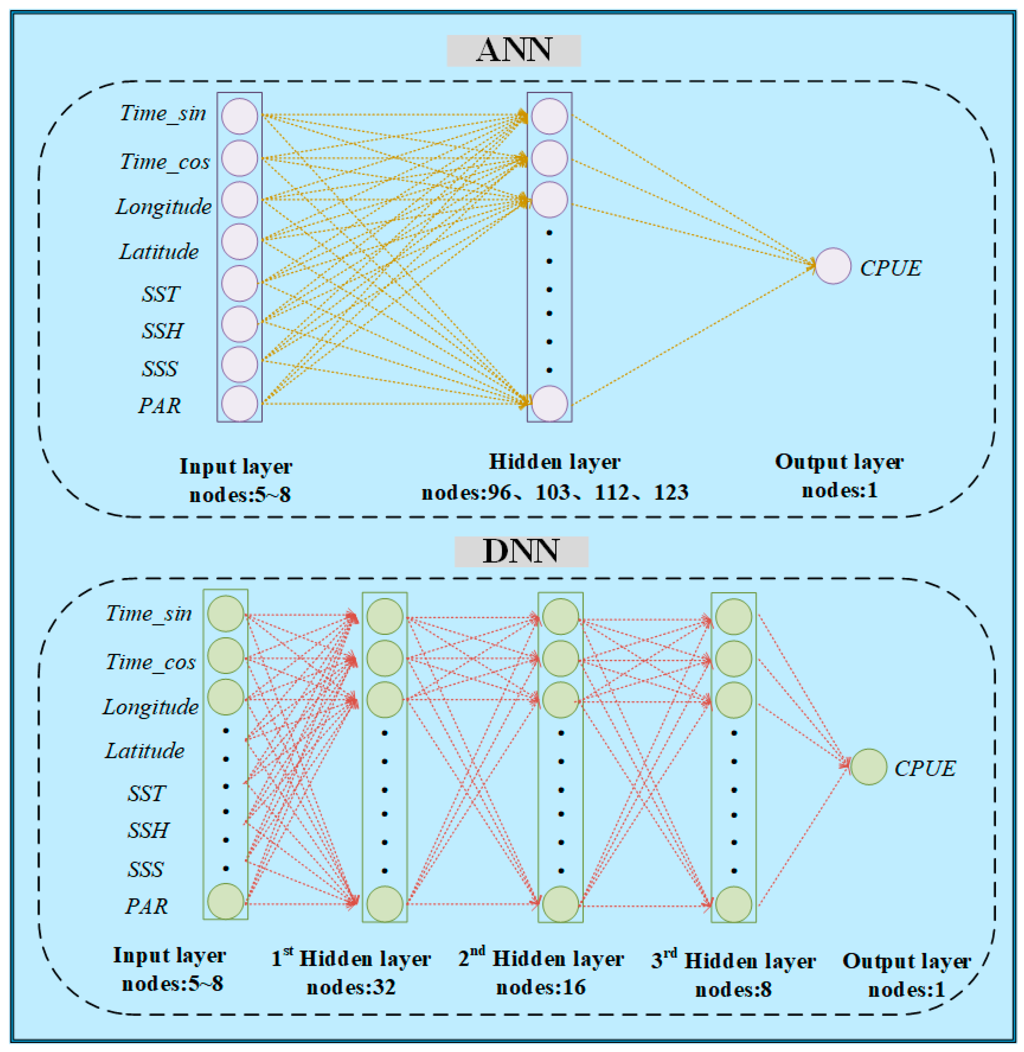
2.3.3. Artificial Neural Network (ANN) and Deep Neural Network (DNN)

Artificial neural network (ANN) is a foundational model in machine learning. It is composed of interconnected neurons organized into input, hidden, and output layers. Through the process of backpropagation, the model continuously adjusts the weights of the error gradients to extract meaningful features from the data, thereby addressing the complex nonlinear relationships between inputs and outputs. Previous research indicated that the performance of traditional ANN models, often with a single hidden layer, is significantly influenced by the number of neurons in that layer [39]. Researchers typically design the number of neurons through empirical methods to find the optimal solution, a process that can be time-consuming.

However, deep learning enhances model capacity by increasing the dimensionality, incorporating multiple hidden layers to explore deeper data features, and thus efficiently and reliably executing complex nonlinear regression tasks [40,41]. The deep fully connected neural network, referred to as the DNN model, is a typical deep learning model. It is built with multiple hidden layers. Through the training process across multiple hidden layers, the model can extract higher-order, more abstract features, enhancing its representational and generalization capabilities. In this study, the DNN model’s input layer included combinations of different environmental factors with 5 to 8 neurons, followed by three hidden layers with 32, 16, and 8 neurons, respectively. The output layer consisted of a single neuron representing the CPUE. To ensure a fair comparison between the two models, the number of parameters was kept consistent. The number of neurons in the ANN’s hidden layer was adjusted according to the input layer, and ranged from 96 to 103 to 112 to 123 neurons (Figure 3). Since the output CPUE was greater than zero, the ReLU activation function was employed.

2.4. Model Evaluation Parameters

In regression tasks within machine learning, model accuracy is typically evaluated using metrics such as mean square error (MSE) and mean absolute error (MAE). The formulas are defined as follows [42]:

$$\mathit{MSE}={\displaystyle \frac{1}{n}}{\sum }_{i=1}^n{(y_i-{\widehat{y}}_i)}^2$$

(6)

$$\mathit{MAE}={\displaystyle \frac{1}{n}}{\sum }_{i=1}^n\left|y_i-{\widehat{y}}_i\right|$$

(7)

where “$y_i$” represents the actual CPUE value, “${\widehat{y}}_i$” represents the predicted CPUE value, and “n” denotes the sample size.

The CPUE distribution on fishing ground often exhibits a sparse, scattered pattern with a significant number of zeros, especially at relatively fine temporal scales, and the MSE and MAE may not accurately capture the spatiotemporal distribution of the CPUE. Therefore, the effectiveness of the model was further evaluated by calculating the area under the precision−recall (P−R) curve (AUC). The threshold values were generated starting from 0 up to the maximum predicted CPUE value at the current temporal scale, incrementing by 5% quantiles. The formula is as follows [43]:

$$\mathit{AUC}={\sum }_{i=1}^{n-1}{\displaystyle \frac{{(Recall}_{i+1}-{Recall}_i)\times {(Precision}_{i+1}+{Precision}_i)}{2}}$$

(8)

$$Precision={\displaystyle \frac{N_{TP}}{N_{TP}+N_{FP}}}$$

(9)

$$Recall={\displaystyle \frac{N_{TP}}{N_{TP}+N_{FN}}}$$

(10)

where “N_TP” represents the number of true positives, “N_FP” represents the number of false positives, “N_FN” represents the number of false negatives, and “n” is the number of thresholds in the sequence.

2.5. Model Implementation

To ensure a fair comparison of model performance, all the models were trained in a consistent environment. The graphics processing unit (GPU) used in this study was an NVIDIA GeForce RTX 2080 Ti, running on a Linux operating system. The models were implemented using the TensorFlow 2.4.1 framework with Python 3.7. The data from 2012 to 2020 were split into training and validation sets at a 4:1 ratio for cross-validation to optimize the model parameters. The samples from 2021 were set aside as the test set.

2.6. Interpretability of Model Input Factors

SHAP (Shapley additive explanations) is a game theoretic approach to explaining the output of any machine learning model. It connects optimal credit allocation with local explanations using the classic Shapley values from game theory and their related extensions [44]. The influence of non-zero impact factors within the model can be quantified by calculating the prediction differences before and after their removal. This method is particularly effective for enhancing the interpretability of deep learning networks with complex architectures [45]. In this study, Case 8 included the largest number of input factors, totaling eight. Therefore, this case was selected to analyze the influence of each spatiotemporal and environmental factor on the prediction model’s output.

3. Results

3.1. MSE and MAE of Different Models

The accuracy of each model under multiple temporal scales, which was based on the optimal environmental factor combinations, is illustrated in Figure 4. Both the MSE and MAE showed consistent trends. The MSE ranged from 15.96 to 30.75, whereas the MAE ranged from 2.71 to 3.91. The best performing model across all the cases was the DNN model at the 30-day temporal scale. For all temporal scales, the DNN model consistently presented the lowest MSE and MAE values, followed by the ANN, XGBoost, and GAM models. Based on the average value of all models, both the MSE and MAE increased as the temporal scale became finer, indicating a decline in model performance. Additionally, the variance among the models decreased, with MSE ranging from 1.52 to 0.84 and MAE ranging from 0.23 to 0.10. This suggests that the performance differences among the models were greatest at the 30-day temporal scale and diminished as the temporal scale decreased.

3.2. AUC Evaluation of P-R Curves

The AUC of the P-R curve effectively demonstrates the CPUE spatiotemporal distribution fitting performance across different quantile threshold series for various models. As shown in Figure 5, the AUC for each model across multiple temporal scales revealed that the ANN and DNN models outperformed the GAM and XGBoost. As the temporal scale decreased, the AUC values for all the models also decreased, with a range from 0.017 to 0.079. The highest AUC was achieved by the DNN model at the 30-day temporal scale, which was consistent with the trends observed in MSE and MAE. Across all temporal scales, the DNN model consistently delivered the best AUC performance. While the ANN model underperformed at the 30-day scale, it generally outperforms the GAM and XGBoost at other temporal scales.

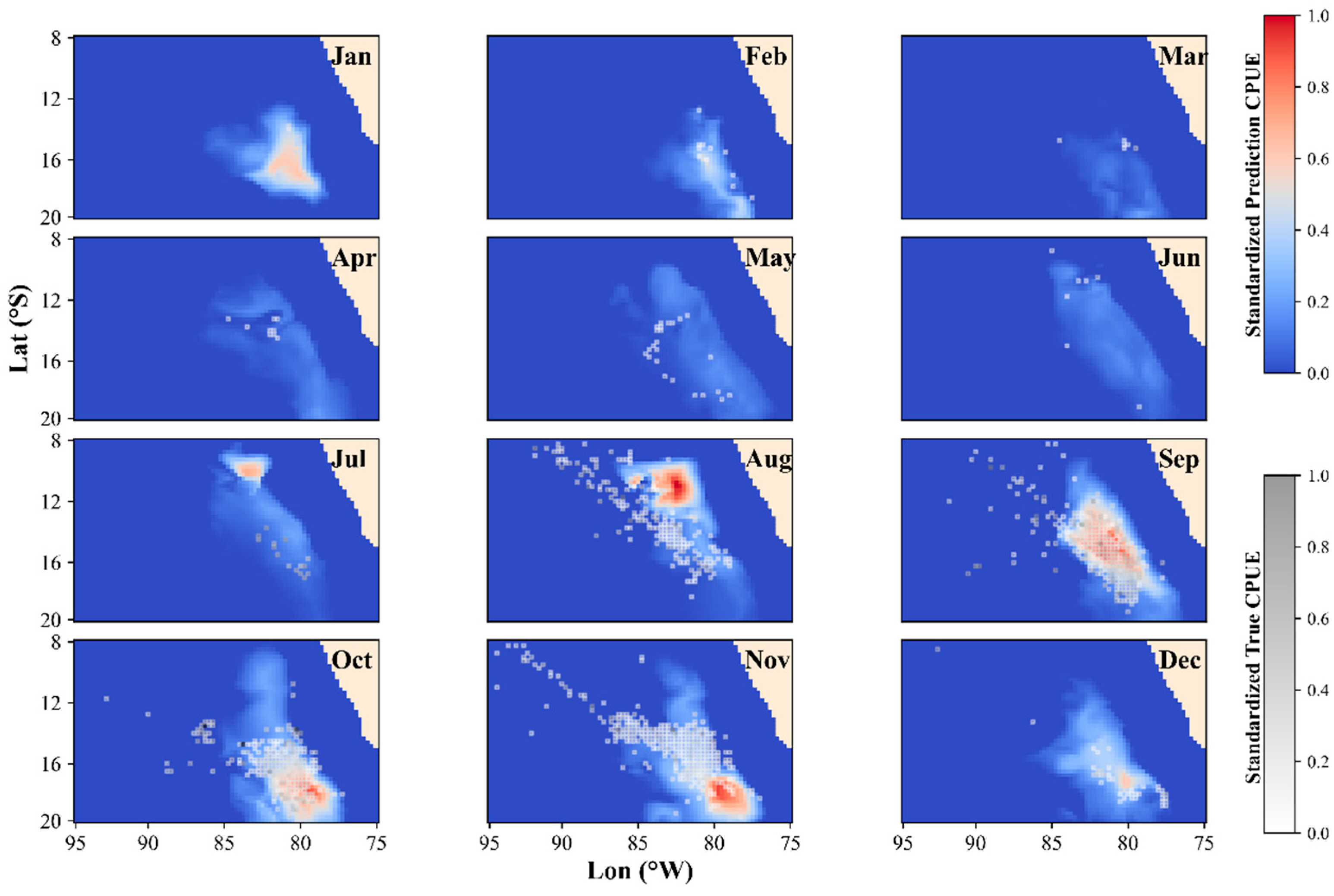
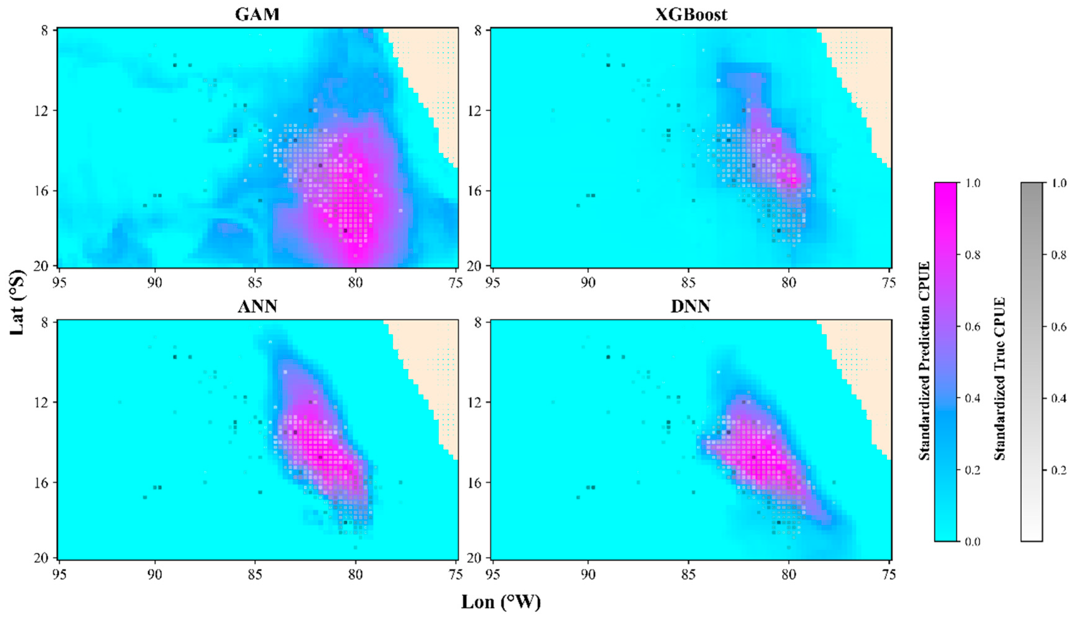
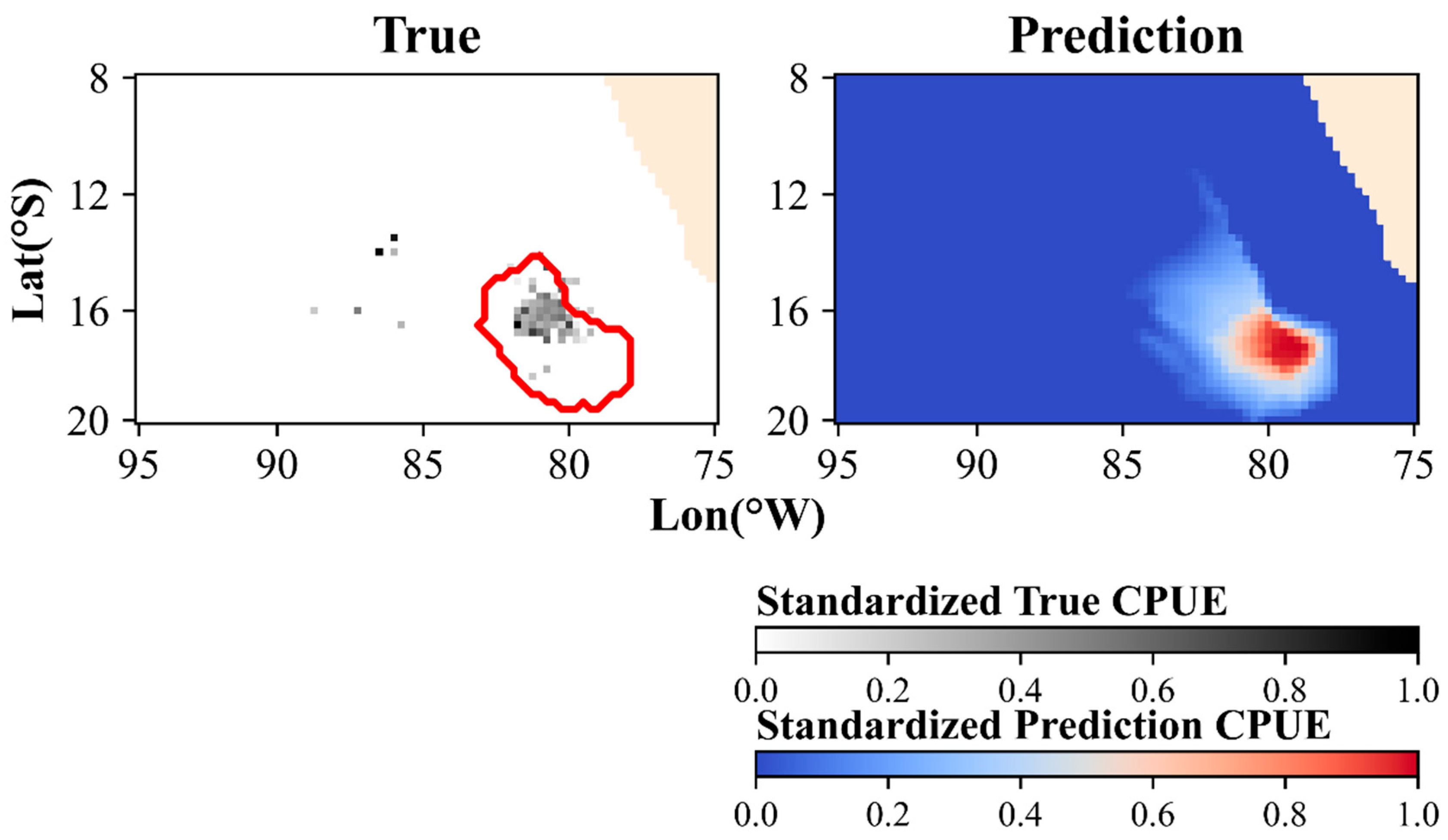
3.3. Spatiotemporal Distribution in the Optimal Model

The optimal model across all the cases was the DNN model with a 30-day temporal scale. To evaluate the model’s predictive performance, the predicted spatiotemporal distribution from the test set was overlaid with the actual CPUE portions. As shown in Figure 6, the DNN model effectively captured the contours of the actual CPUE portions and distinguished between different months. In months with lower CPUE portions, the predicted fishing grounds were correspondingly smaller. During the months with higher CPUE values, such as August to November, the predicted fishing grounds largely overlapped with the actual CPUE portions. However, there was some degree of spatial displacement in the high CPUE regions, particularly in terms of latitude during July and November.

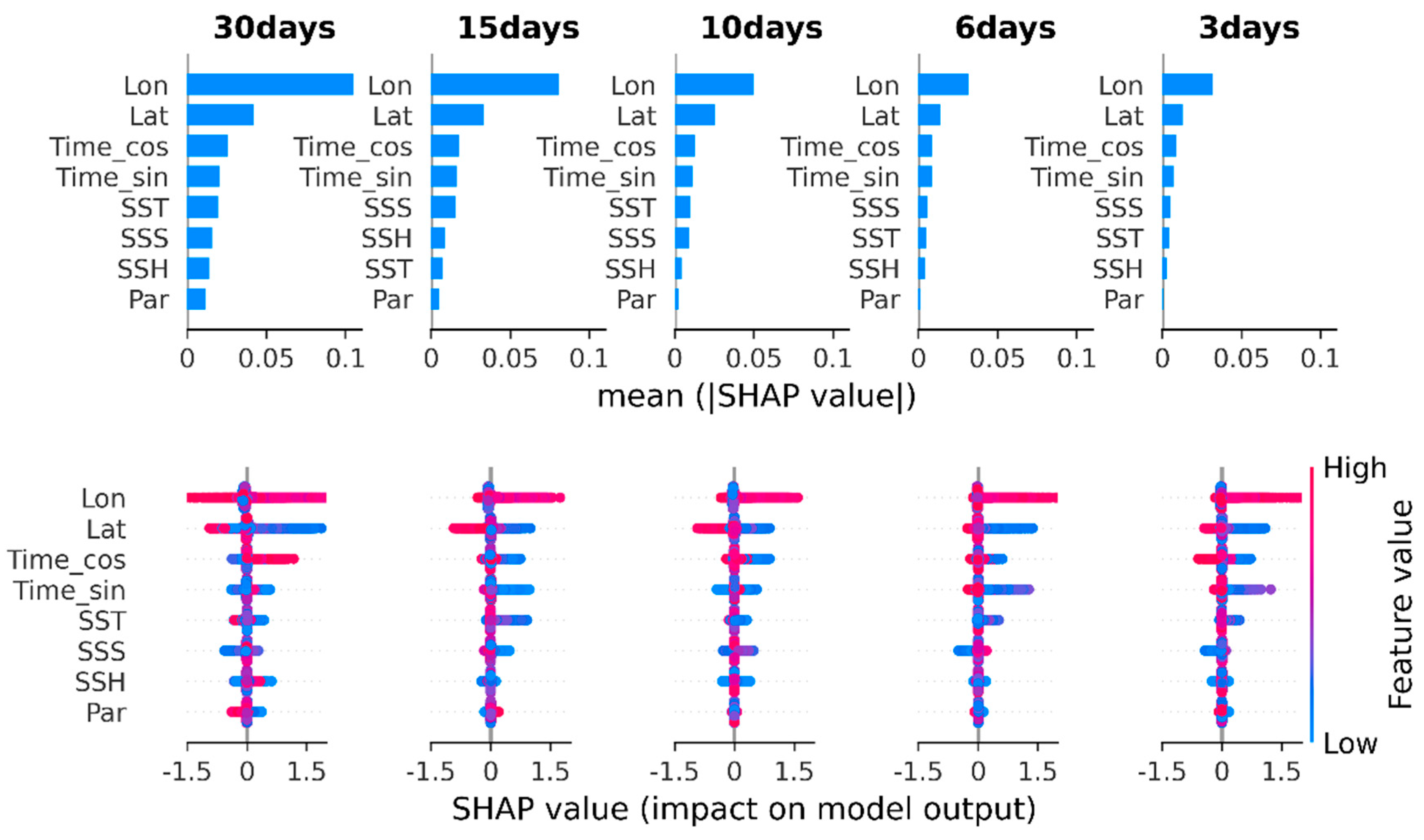
3.4. Shapley Additive Explanation of Model Predictions

Based on the SHAP value results across different temporal scales (Figure 7), the top four input factors in all cases exhibited the same ranking of contributions: Lon, Lat, Time_cos, and Time_sin, with Lon showing the highest contribution, significantly surpassing the other factors. The ranking of the remaining four factors varied, with Par consistently contributing the least. Additionally, the overall contribution of these factors decreased as the temporal scale becomes finer.

4. Discussion

4.1. Performance Comparison of Different Models

On the basis of the model performance evaluation metrics, including the MSE and MAE, and the AUC of the P−R curve, the DNN model outperformed the other models (Figure 4 and Figure 5). The 30-day temporal scale was the optimal temporal scale for all models. As shown by the monthly average CPUE of Dosidicus gigas in the Southeast Pacific (Figure 8), the months with higher CPUE occurred in the second half of the year, indicating significant seasonal variation. Therefore, we selected September 2021 as an example to compare and analyze the differences in the spatiotemporal distribution of Dosidicus gigas among the four models.

For the GAM and ANN models, the optimal environmental factor combination was SST, SSS, and PAR; for XGBoost, it was SST; and for DNN, it was SST and SSS. The predicted spatial distribution for each model based on the optimal environmental factor combinations was superimposed with the actual CPUE. As shown in the comparison results (Figure 9), all models were able to simulate the spatial distribution of Dosidicus gigas. However, the GAM model predicted a larger spatial range with blurred edges, resulting in the worst performance in terms of both the MSE and the AUC of the P−R curve. Compared with the GAM, the XGBoost model significantly reduced the predicted fishing ground area, with a more concentrated center fishing ground. However, the edges were not smooth, showing rectangular variation, possibly due to the greater influence of spatial factors (longitude and latitude). Compared with the previous two models, the ANN and DNN models clearly distinguished zero values from nonzero values, leading to very clear prediction of fishing ground boundaries. This was related to the use of the ReLU function in the last layer of the neural network. Additionally, during the training process, neural networks update weights through the backpropagation algorithm, allowing these weights to learn which features in the input data are more important for distinguishing zero values from nonzero values [46]. Compared with the ANN, the DNN model predicted a more concentrated center fishing ground, with a smaller area and a dimensionality closer to the actual nominal CPUE. This is because deep learning, with its multilayer hidden structure, better captures the complex features of the data. The extraction of high-level features layer by layer, further improves the prediction performance [47]. In this study, model comparisons were conducted for a single species only. However, oceanic cephalopods tend to exhibit greater spatial distribution similarities driven by marine environmental factors. Future research will explore comparative analyses between transfer learning and inter-model performance using case studies of other species (e.g., Ommastrephes bartramii in the Pacific Ocean) to evaluate the effectiveness of transfer learning in enhancing model performance.

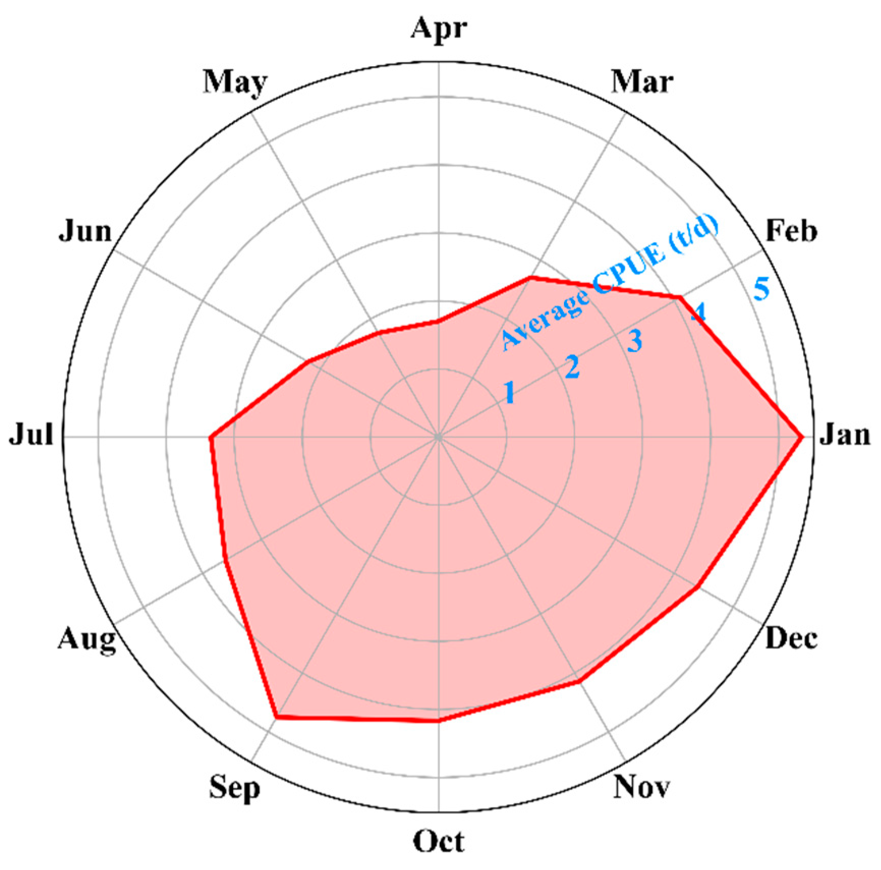
4.2. Differences Across Temporal Scales

In previous studies on the spatiotemporal distribution of pelagic economic species, the temporal scales were predominantly annual and monthly [39,48]. This is primarily because pelagic species are significantly influenced by oceanic climate changes, with marine environmental factors exhibiting marked seasonal variations, leading to the distinct seasonal migrations of these species. The cycles of these oceanic climate and environmental changes generally align with annual or monthly scales [49,50].

Moreover, most distant-water fishery data originate from commercial fishing vessels, where the operational costs, including fuel, labor, and maintenance costs, are quite high. Therefore, only at larger temporal scales can catch data accumulate sufficiently to enable statistical analysis. However, with advancements in ocean remote sensing and distant-water fishery technology, the data volume has increased significantly, ushering in the “big data” era, thereby increasing the demand for finer temporal scales and greater precision in distant-water fisheries.

To increase the quality and timeliness of fishery forecasts, this study adopted finer temporal scales, including 30 days, 15 days, 10 days, 6 days, and 3 days, to explore the model’s performance changes and limitations. The results indicated that as the temporal scale decreased, model performance deteriorated (Figure 4 and Figure 5). From a machine learning perspective, reducing the temporal scale should improve model performance due to an increase in sample size (Table 1). However, the opposite was observed, which can be attributed to the corresponding increase in noise and interference in the samples. For instance, in September 2021 (Figure 10), when the temporal scale was 30 days, the number of sites with actual CPUE values was sufficient, forming a distinct center fishing ground. As the temporal scale decreased, the CPUE portions from multiple periods became more dispersed, and the predicted center fishing ground area decreased, leading to varying degrees of prediction bias. At finer scales, such as 3 days, the environmental factors showed minimal variation across the 10 periods, resulting in insignificant changes in the predicted center fishing ground across periods. However, the spatial distribution of the actual CPUE values differed significantly, making the model’s performance at the 3-day scale the poorest.

Notably, models such as the GAM, when predicting at a 3-day scale, still forecast a large center fishing ground area, indicating that traditional statistical models struggled with more refined temporal scale prediction tasks. In months with higher CPUE values (the second half of the year), the predicted results generally covered the actual CPUE sites. However, in months with lower yields (the first half of the year), at the 3-day scale, there were many periods with little to no actual CPUE sites, introducing significant noise and interference into the model’s predictions. Therefore, merely increasing the sample size without considering quality offers neither fisheries production nor scientific merit. A balance between sample quantity and quality must be achieved. Future research should focus on reducing data noise to improve the precision of temporal-scale predictions of fishing ground distribution.

4.3. Interpretation of Input Factors Effect

In the SHAP analysis of input factors, the contribution of spatiotemporal factors to the model prediction significantly outweighed that of environmental factors. This was primarily because Dosidicus gigas, as a migratory species, exhibited a pronounced seasonal spatial distribution. Its life history involves a northward feeding migration during summer and fall, followed by a return to the Mexican coast for spawning in late fall or early winter [51,52]. Consequently, longitude and latitude demonstrated the highest contributions.

However, the input factors are autocorrelated with each other. Environmental factors such as SST also affect the contribution of longitude and latitude. And SST also display significant seasonal variations. Because the predictive performance of the model reflects the combined effects of multiple factors, which SHAP analysis cannot fully disentangle. The contribution of all input factors diminished as the temporal scale decreased (Figure 7), suggesting that at finer temporal resolutions, the variability in the spatial and temporal distribution of the fisheries data became less pronounced. This may be attributed to the discrete and sparse nature of the data, which complicates species distribution modeling. Therefore, the modeled relationships between input and output factors alone may not have sufficiently captured differences across periods. Future research at finer temporal scales may benefit from integrating a priori knowledge-based data-preprocessing to enhance the distinction between periods. Additionally, the minimal contribution of PAR might be explained by the close association of primary productivity with the early life history of Dosidicus gigas, which does not closely align with real-time fishing ground distribution patterns.

4.4. The Challenge of Presence-Only Data in SDM

The species distribution model (SDM) can adopt different modeling approaches depending on the type of data and research objectives. In this study, the fisheries catch data were presence-only, meaning that data were only available for locations where CPUE records existed [53]. This indicates that the records captured both the presence of CPUE locations and the associated catch and effort values, from which the CPUE could be calculated. However, absence records do not necessarily imply a lack of catch. Rather, they might indicate areas with environmental conditions suitable for capture, but where fishing was not conducted owing to factors such as weather conditions or decisions made by the fishing vessel’s crew. This characteristic of pelagic fishery data makes it unsuitable for many commonly used SDMs.

Previous spatial distribution prediction studies have typically overlooked this issue. This oversight is partly because those studies often employed larger temporal scales than the present study did, allowing statistical models to effectively handle unsampled portions of data. For example, in tuna research, when both the spatial and temporal scales are sufficiently large, the aggregation of the center fishing ground is pronounced, and the noise from missing data has a minimal impact on the model. However, in the study of Dosidicus gigas, the smaller temporal scales exacerbated the negative impact of unsampled portions caused by presence-only data, significantly degrading model accuracy. The model’s predictions were consistently smooth and continuous, making it impossible to predict discrete zero-value points within these smooth regions (Figure 11), unless pseudo absences were assigned to unsampled portions of the center fishing ground [54,55].

Therefore, we should focus on data cleaning and annotating unsampled portions for finer temporal scales. In the present study, spatial distribution modeling of Dosidicus gigas still employed regression methods used in previous studies. Although deep learning can effectively distinguish between zero and nonzero values, the predicted CPUE values within the nonzero regions still differed in scale from the actual CPUE, primarily because the presence-only nature of the data was not considered, and zero values were treated as part of the regression task. Future research will diverge from this approach, employing a one-class classifier to first differentiate between zero and nonzero values, and then performing regression within the cleaned nonzero regions to improve the accuracy of spatial distribution prediction at finer temporal scales.

5. Conclusions

This study developed spatial distribution models for Dosidicus gigas in the Southeast Pacific at multiple temporal scales. A novel deep learning-based approach was proposed, and the results demonstrated that this model outperformed other traditional models. As the temporal scale decreased, both the MSE and MAE increased, whereas the AUC of the P−R curve decreased, indicating a decline in model performance. The DNN model effectively predicted the contours of the actual CPUE, with noticeable distinctions between periods. Compared with the GAM and XGBoost models, the DNN model provided sharper boundaries around the core fishing grounds. It also demonstrated more concentrated and smaller areas of prediction than did the neural network model. The SHAP analysis indicated that spatial and temporal factors significantly contributed to the model, with longitude exhibiting the highest contribution.

The decline in model performance with finer temporal scales can likely be attributed to the presence of many periods with few or no actual CPUE portions. These periods introduce significant noise and interference in the model’s prediction. Thus, merely increasing the sample size without considering the quality is neither productive for fisheries management nor scientifically meaningful. A balance between sample quantity and quality is essential. A limitation of this study was that it focused on a single species, which may have introduced substantial stochastic variability. Future research should encompass a broader range of oceanic economic species and incorporate comparative analyses to improve the robustness and generalizability of the model findings. It should also focus on denoising the data and addressing the presence-only nature of fisheries data by employing a one-class classifier to clean unsampled portions of the core fishing ground. Additionally, efforts should be directed toward identifying and incorporating key environmental variables that exert greater influence on SDMs to enhance model performance.

References

1. Chen, X.; Liu, B.; Chen, Y. A review of the development of Chinese distant-water squid jigging fisheries. Fish. Res. 2008, 89, 211–221. [Google Scholar] [CrossRef]
2. Rocha, F.; Vega, M.A. Overview of cephalopod fisheries in Chilean waters. Fish. Res. 2003, 60, 151–159. [Google Scholar] [CrossRef]
3. Chen, X. Theory and Method of Fisheries Forecasting; Springer Nature: Singapore, 2022. [Google Scholar]
4. Xiang, D.; Li, Y.; Jiang, K.; Han, H.; Wang, Y.; Yang, S.; Zhang, H.; Sun, Y. Environmental influences on Illex argentinus trawling grounds in the southwest Atlantic high seas. Fishes 2024, 9, 209. [Google Scholar] [CrossRef]
5. Yu, W.; Chen, X. Ocean warming-induced range-shifting of potential habitat for jumbo flying squid Dosidicus gigas in the Southeast Pacific Ocean off Peru. Fish. Res. 2018, 204, 137–146. [Google Scholar] [CrossRef]
6. Tafur, R.; Keyl, F.; Argüelles, J. Reproductive biology of jumbo squid Dosidicus gigas in relation to environmental variability of the northern Humboldt Current System. Mar. Ecol. Prog. Ser. 2010, 400, 127–141. [Google Scholar] [CrossRef]
7. Keyl, F.; Argüelles, J.U.A.N.; Mariategui, L.; Tafur, R.; Wolff, M.; Yamashiro, C. A hypothesis on range expansion and spatio-temporal shifts in size-at-maturity of jumbo squid (Dosidicus gigas) in the Eastern Pacific Ocean. CalCOFI Rep. 2008, 49, 119–128. [Google Scholar]
8. Fang, X.; Zhang, Y.; Yu, W.; Chen, X. Geographical distribution variations of Humboldt squid habitat in the Eastern Pacific Ocean. Ecosyst. Health Sustain. 2023, 9, 10. [Google Scholar] [CrossRef]
9. Wu, X.; Jin, P.; Zhang, Y.; Yu, W. Spatial Distribution and Abundance of a Pelagic Squid during the Evolution of Eddies in the Southeast Pacific Ocean. J. Mar. Sci. Eng. 2024, 12, 1015. [Google Scholar] [CrossRef]
10. Yu, W.; Yi, Q.; Chen, X.; Chen, Y. Modelling the effects of climate variability on habitat suitability of jumbo flying squid, Dosidicus gigas, in the Southeast Pacific Ocean off Peru. ICES J. Mar. Sci. 2016, 73, 239–249. [Google Scholar] [CrossRef]
11. Jia, S.; Bei, L.; Li, Y.; Zhao, Q. Spatiotemporal analysis of ocean primary productivity in Bohai Sea estimated using improved DINEOF reconstructed MODIS data. Ecol. Inform. 2024, 84, 102920. [Google Scholar] [CrossRef]
12. Medellín-Ortiz, A.; Cadena-Cárdenas, L.; Santana-Morales, O. Environmental effects on the jumbo squid fishery along Baja California’s west coast. Fish. Sci. 2016, 82, 851–861. [Google Scholar] [CrossRef]
13. Castillo, R.; Dalla Rosa, L.; García Diaz, W.; Madureira, L.; Gutierrez, M.; Vásquez, L.; Koppelmann, R. Anchovy distribution off Peru in relation to abiotic parameters: A 32-year time series from 1985 to 2017. Fish. Oceanogr. 2019, 28, 389–401. [Google Scholar] [CrossRef]
14. Armas, E.; Arancibia, H.; Neira, S.; Marín, M.C. Neural network approach for detecting spatial changes in catch probability of Engraulis ringens during El Niño-Southern Oscillation events in northern Chile. Fish. Oceanogr. 2024, 33, e12672. [Google Scholar] [CrossRef]
15. Poisson, F.; Ellis, J.R.; McCully Phillips, S.R. Preliminary Insights on the Habitat Use and Vertical Movements of the Pelagic Stingray (Pteroplatytrygon violacea) in the Western Mediterranean Sea. Fishes 2024, 9, 238. [Google Scholar] [CrossRef]
16. Xie, M.; Liu, B.; Chen, X. Deep learning-based fishing ground prediction with multiple environmental factors. Mar. Life Sci. Technol. 2024, 6, 736–749. [Google Scholar] [CrossRef]
17. Catalano, G.A.; D’Urso, P.R.; Arcidiacono, C. Predicting potential biomass production by geospatial modelling: The case study of citrus in a Mediterranean area. Ecol. Inform. 2024, 83, 102848. [Google Scholar] [CrossRef]
18. Ribeiro, M.C.; Pinho, P.; Llop, E.; Branquinho, C.; Sousa, A.J.; Pereira, M.J. Multivariate geostatistical methods for analysis of relationships between ecological indicators and environmental factors at multiple spatial scales. Ecol. Indic. 2013, 29, 339–347. [Google Scholar] [CrossRef]
19. Wang, J.; Chen, X.; Li, Y.; Boenish, R. The effects of climate-induced environmental variability on Pacific Ocean squids. ICES J. Mar. Sci. 2023, 80, 878–888. [Google Scholar] [CrossRef]
20. Li, X.; Liu, B.; Zheng, G.; Ren, Y.; Zhang, S.; Liu, Y.; Gao, L.; Liu, Y.; Zhang, B.; Wang, F. Deep-learning-based information mining from ocean remote-sensing imagery. Natl. Sci. Rev. 2020, 7, 1584–1605. [Google Scholar] [CrossRef]
21. Rubbens, P.; Brodie, S.; Cordier, T.; Destro Barcellos, D.; Devos, P.; Fernandes-Salvador, J.A.; Fincharm, J.I.; Gomes, A.; Handegard, N.O.; Howell, K.; et al. Machine learning in marine ecology: An overview of techniques and applications. ICES J. Mar. Sci. 2023, 80, 1829–1853. [Google Scholar] [CrossRef]
22. Landy, J.C.; Dawson, G.J.; Tsamados, M.; Bushuk, M.; Stroeve, J.C.; Howell, S.E.; Krumpen, T.; Babb, D.G.; Komarov, A.S.; Heorton, H.D.; et al. A year-round satellite sea-ice thickness record from CryoSat-2. Nature 2022, 609, 517–522. [Google Scholar] [CrossRef] [PubMed]
23. Tupan, J.M.; Rieuwpassa, F.; Setha, B.; Latuny, W.; Goesniady, S. A Deep Learning Approach to Automated Treatment Classification in Tuna Processing: Enhancing Quality Control in Indonesian Fisheries. Fishes 2025, 10, 75. [Google Scholar] [CrossRef]
24. Kroodsma, D.A.; Mayorga, J.; Hochberg, T.; Miller, N.A.; Boerder, K.; Ferretti, F.; Wilson, A.; Bergman, B.; White, T.D.; Block, B.A.; et al. Tracking the global footprint of fisheries. Science 2018, 359, 904–908. [Google Scholar] [CrossRef]
25. Song, Y.; Zhang, S.; Tang, F.; Shi, Y.; Wu, Y.; He, J.; Chen, Y.; Li, L. Behavior Recognition of Squid Jigger Based on Deep Learning. Fishes 2023, 8, 502. [Google Scholar] [CrossRef]
26. Wu, X.; Jin, P.; Zhang, Y.; Yu, W. Changing Humboldt Squid Abundance and Distribution at Different Stages of Oceanic Mesoscale Eddies. J. Mar. Sci. Eng. 2024, 12, 626. [Google Scholar] [CrossRef]
27. Yu, W.; Feng, X.; Wen, J.; Wu, X.; Fang, X.; Cui, J.; Feng, Z.; Sheng, Y.; Zhao, Z.; Liu, B.; et al. The potential impacts of climate change on the life history and habitat of jumbo flying squid in the southeast Pacific Ocean: Overview and implications for fisheries management. Rev. Fish Biol. Fisher. 2025, 35, 707–731. [Google Scholar] [CrossRef]
28. Tian, S.; Chen, X.; Chen, Y.; Xu, L.; Dai, X. Standardizing CPUE of Ommastrephes bartramii for Chinese squid-jigging fishery in Northwest Pacific Ocean. Chin. J. Oceanol. Limn. 2009, 27, 729–739. [Google Scholar] [CrossRef]
29. Paulino, C.; Segura, M.; Chacón, G. Spatial variability of jumbo flying squid (Dosidicus gigas) fishery related to remotely sensed SST and chlorophyll-a concentration (2004–2012). Fish. Res. 2016, 173, 122–127. [Google Scholar] [CrossRef]
30. Xie, Y.; Zhong, Z.; Li, B.; Xie, Y.; Chen, L.; Chen, H. An ARM-FPGA Hybrid Acceleration and Fault Tolerant Technique for Phase Factor Calculation in Spaceborne Synthetic Aperture Radar Imaging. IEEE J. Sel. Top. Appl. Earth Obs. Remote. Sens. 2024, 17, 5059–5072. [Google Scholar] [CrossRef]
31. Shi, Y.; Zhang, X.; Yang, S.; Dai, Y.; Cui, X.; Wu, Y.; Zhang, S.; Fan, W.; Han, H.; Zhang, H.; et al. Construction of CPUE standardization model and its simulation testing for chub mackerel (Scomber japonicus) in the Northwest Pacific Ocean. Ecol. Indic. 2023, 155, 111022. [Google Scholar] [CrossRef]
32. Uzer, U. Influence of Environmental Parameters on the Abundance of Tub Gurnard, Chelidonichthys lucerna, in the Eastern Sea of Marmara. Fishes 2025, 10, 127. [Google Scholar] [CrossRef]
33. Wang, L.; Yang, C.; Shan, B.; Liu, Y.; Zou, J.; Sun, D.; Guo, T. Spatiotemporal Variation and Predictors of the Purpleback Flying Squid (Sthenoteuthis oualaniensis) Distribution Surrounding the Xisha and Zhongsha Islands during a Fishing Moratorium. Fishes 2024, 9, 253. [Google Scholar] [CrossRef]
34. Hamzaoui, M.; Aoueileyine, M.O.E.; Romdhani, L.; Bouallegue, R. Optimizing XGBoost performance for fish weight prediction through parameter pre-selection. Fishes 2023, 8, 505. [Google Scholar] [CrossRef]
35. Xing, B.; Zhang, L.; Liu, Z.; Sheng, H.; Bi, F.; Xu, J. The study of fishing vessel behavior identification based on ais data: A case study of the east China sea. J. Mar. Sci. Eng. 2023, 11, 1093. [Google Scholar] [CrossRef]
36. Xu, S.; Wang, J.; Chen, X.; Zhu, J. Identifying optimal variables for machine-learning-based fish distribution modeling. Can. J. Fish. Aquat. Sci. 2024, 81, 687–698. [Google Scholar] [CrossRef]
37. Chen, B.; Mu, X.; Chen, P.; Wang, B.; Choi, J.; Park, H.; Xu, S.; Wu, Y.; Yang, H. Machine learning-based inversion of water quality parameters in typical reach of the urban river by UAV multispectral data. Ecol. Indic. 2021, 133, 108434. [Google Scholar] [CrossRef]
38. Yang, W.; Fu, B.; Li, S.; Lao, Z.; Deng, T.; He, W.; He, H.; Chen, Z. Monitoring multi-water quality of internationally important karst wetland through deep learning, multi-sensor and multi-platform remote sensing images: A case study of Guilin, China. Ecol. Indic. 2023, 154, 110755. [Google Scholar] [CrossRef]
39. Lin, H.; Wang, J.; Zhu, J.; Chen, X. Evaluating the impacts of environmental and fishery variability on the distribution of bigeye tuna in the Pacific Ocean. ICES J. Mar. Sci. 2023, 80, 2642–2656. [Google Scholar] [CrossRef]
40. Kunimatsu, S.; Kurota, H.; Muko, S.; Ohshimo, S.; Tomiyama, T. Predicting unseen chub mackerel densities through spatiotemporal machine learning: Indications of potential hyperdepletion in catch-per-unit-effort due to fishing ground contraction. Ecol. Inform. 2024, 85, 102944. [Google Scholar] [CrossRef]
41. Zou, S.; Zhang, L.; Huang, X.; Osei, F.B.; Ou, G. Early ecological security warning of cultivated lands using RF-MLP integration model: A case study on China’s main grain-producing areas. Ecol. Indic. 2022, 141, 109059. [Google Scholar] [CrossRef]
42. Burton, M.L.; Potts, J.C.; Ostrowski, A.D. Preliminary estimates of age, growth and natural mortality of margate, Haemulon album, and black margate, Anisotremus surinamensis, from the southeastern United States. Fishes 2019, 4, 44. [Google Scholar] [CrossRef]
43. Gu, K.; Chen, Y. YOLOv3-MSSA based hot spot defect detection for photovoltaic power stations. J. Meas. Eng. 2024, 12, 23–39. [Google Scholar] [CrossRef]
44. Štrumbelj, E.; Kononenko, I. Explaining prediction models and individual predictions with feature contributions. Knowl. Inf. Syst. 2014, 41, 647–665. [Google Scholar] [CrossRef]
45. Shrikumar, A.; Greenside, P.; Kundaje, A. Learning important features through propagating activation differences. In Proceedings of the International Conference on Machine Learning, Sydney, Australia, 6–11 August 2017; pp. 3145–3153. [Google Scholar]
46. Jamei, M.; Ali, M.; Malik, A.; Rai, P.; Karbasi, M.; Farooque, A.A.; Yaseen, Z.M. Designing a decomposition-based multi-phase pre-processing strategy coupled with EDBi-LSTM deep learning approach for sediment load forecasting. Ecol. Indic. 2023, 153, 110478. [Google Scholar] [CrossRef]
47. Zhang, G.; Wang, M.; Liu, K. Deep neural networks for global wildfire susceptibility modelling. Ecol. Indic. 2021, 127, 107735. [Google Scholar] [CrossRef]
48. Han, H.; Yang, C.; Jiang, B.; Shang, C.; Sun, Y.; Zhao, X.; Xiang, D.; Zhang, H.; Shi, Y. Construction of chub mackerel (Scomber japonicus) fishing ground prediction model in the northwestern Pacific Ocean based on deep learning and marine environmental variables. Mar. Pollut. Bull. 2023, 193, 115158. [Google Scholar] [CrossRef]
49. Moyano, G.; Plaza, G.; Cerna, F.; Muñoz, A.A. Local and global environmental drivers of growth chronologies in a demersal fish in the south-eastern pacific ocean. Ecol. Indic. 2021, 131, 108151. [Google Scholar] [CrossRef]
50. Reichstein, M.; Camps-Valls, G.; Stevens, B.; Jung, M.; Denzler, J.; Carvalhais, N.; Prabhat, F. Deep learning and process understanding for data-driven Earth system science. Nature 2019, 566, 195–204. [Google Scholar] [CrossRef]
51. Anderson, C.I.; Rodhouse, P.G. Life cycles, oceanography and variability: Ommastrephid squid in variable oceanographic environments. Fish. Res. 2001, 54, 133–143. [Google Scholar] [CrossRef]
52. Tafur, R.; Villegas, P.; Rabí, M.; Yamashiro, C. Dynamics of maturation, seasonality of reproduction and spawning grounds of the jumbo squid Dosidicus gigas (Cephalopoda: Ommastrephidae) in Peruvian waters. Fish. Res. 2001, 54, 33–50. [Google Scholar] [CrossRef]
53. Martínez-Minaya, J.; Cameletti, M.; Conesa, D.; Pennino, M.G. Species distribution modeling: A statistical review with focus in spatio-temporal issues. Stoch. Environ. Res. Risk A 2018, 32, 3227–3244. [Google Scholar] [CrossRef]
54. Barbet-Massin, M.; Jiguet, F.; Albert, C.H.; Thuiller, W. Selecting pseudo-absences for species distribution models: How, where and how many? Methods Ecol. Evol. 2012, 3, 327–338. [Google Scholar] [CrossRef]
55. Iturbide, M.; Bedia, J.; Herrera, S.; del Hierro, O.; Pinto, M.; Gutiérrez, J.M. A framework for species distribution modelling with improved pseudo-absence generation. Ecol. Model. 2015, 312, 166–174. [Google Scholar] [CrossRef]
Figure 1. Spatial distribution of catch per unit effort (CPUE) in Dosidicus gigas fishing ground in the Southeast Pacific.
Fishes 10 00273 g001
Figure 2. Euclidean distance between January and other months under sine−cosine representation.
Fishes 10 00273 g002
Figure 3. Architecture of the artificial neural network (ANN) and deep neural network (DNN) models.
Fishes 10 00273 g003
Figure 4. The mean squared error (MSE) and mean absolute error (MAE) of each model at multiple temporal scales under the optimal combination of environmental factors.
Fishes 10 00273 g004
Figure 5. The area under the precision−recall curve (AUC) for each model at multiple temporal scales.
Fishes 10 00273 g005
Figure 6. Monthly spatial distribution of Dosidicus gigas predicted by the deep neural network (DNN) overlaid with true catch per unit effort (CPUE).
Fishes 10 00273 g006
Figure 7. SHAP values and mean absolute value of environmental factors on prediction models at different temporal scales.
Fishes 10 00273 g007
Figure 8. Monthly mean catch per unit effort (CPUE) of Dosidicus gigas in the southeastern Pacific Ocean.
Fishes 10 00273 g008
Figure 9. Comparison of the spatial distribution prediction results of different models in September 2021.
Fishes 10 00273 g009
Figure 10. Spatial distribution prediction of the deep neural network (DNN) models for each period at multiple temporal scales (Symbols ① to ⑩ represent the order of periods at different temporal scales.).
Fishes 10 00273 g010
Figure 11. Unsampled portions within the predicted area at the 3-day temporal scale (the red circle in the left figure is the central spatial distribution range predicted by the model).
Fishes 10 00273 g011