
Seasonal Trends in Water Retention of Atlantic Sea Cucumber (Cucumaria frondosa): A Modeling Approach


Abstract
1. Introduction
2. Materials and Methods
2.1. Sample Collection and Preparation
2.1.1. Sample Collection from the Vessel
- The following information was collected from the processor or unloading facility supervisor and recorded the following prior to sampling:
- vessel information;
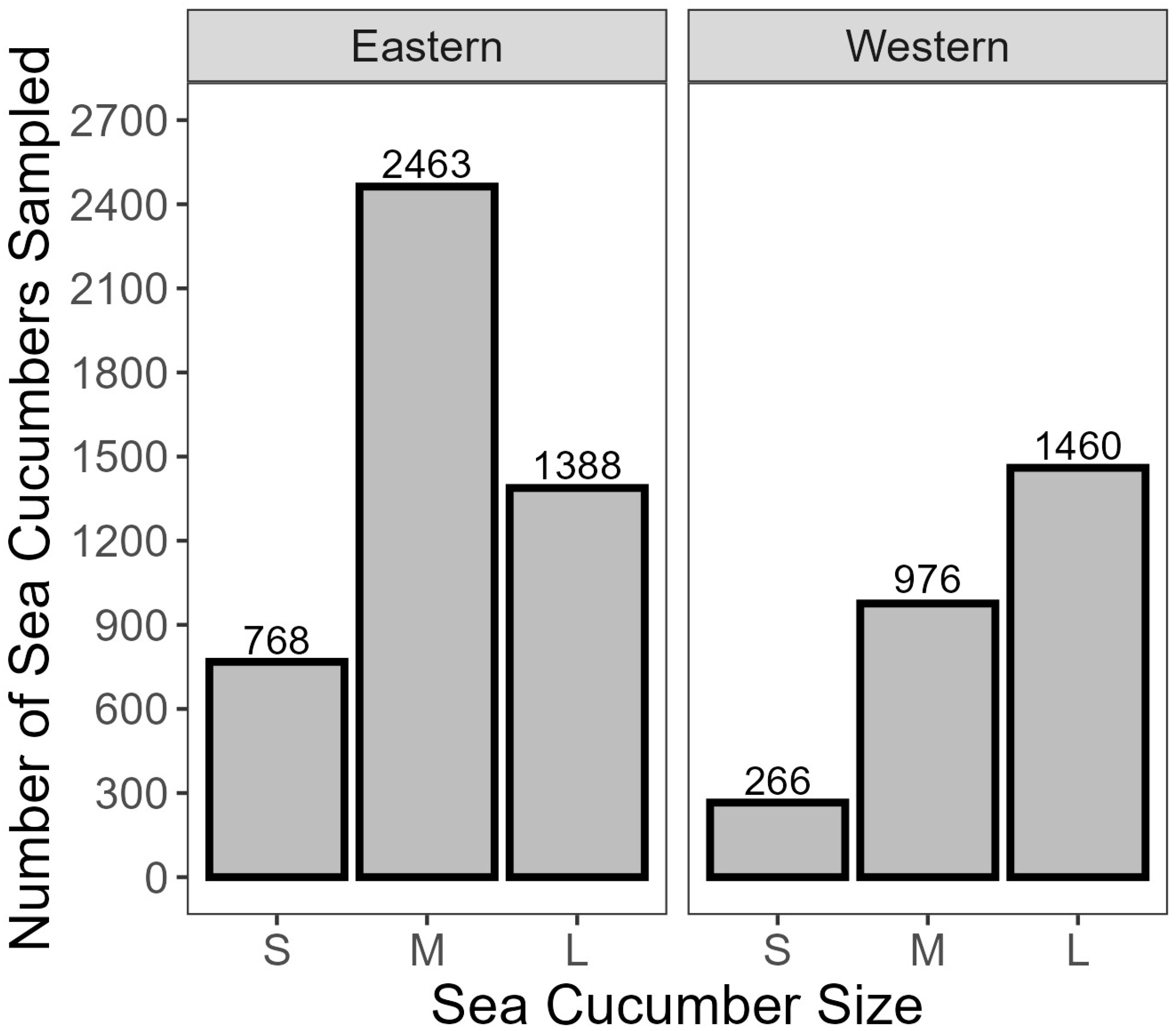
- fishing area;
- hail weight.
- Using the hail weight, the load was divided into top, middle and bottom based on storage position in the boat’s hold.
- Unloading was executed using one of the following two methods, depending on the facility:
- Unloading staff shoveled product into a bucket which was hoisted out of the hold and loaded into a tote (bucket method).
- Sea water was pumped into the hold and product was transferred over a drain screen to the tote using a vacuum pump (vacuum transfer).
- As the vessel was unloaded, the following was undertaken:
- Two 2000 L or three 1000 L insulated totes were randomly selected and identified using Number Generator Random, v 2.1 [20] from each of the top, middle, and bottom sections of the hold.
- Once filled, these totes were segregated and used for sample collection.
- No water was added to the process.
- The Transcell scale was tared for the weight of the Stacknest pans and ~40 kg of sea cucumber samples were randomly transferred from each segregated tote into each pan.
- Each pan was weighed and tagged to identify the collection time, weight, and sampling location.
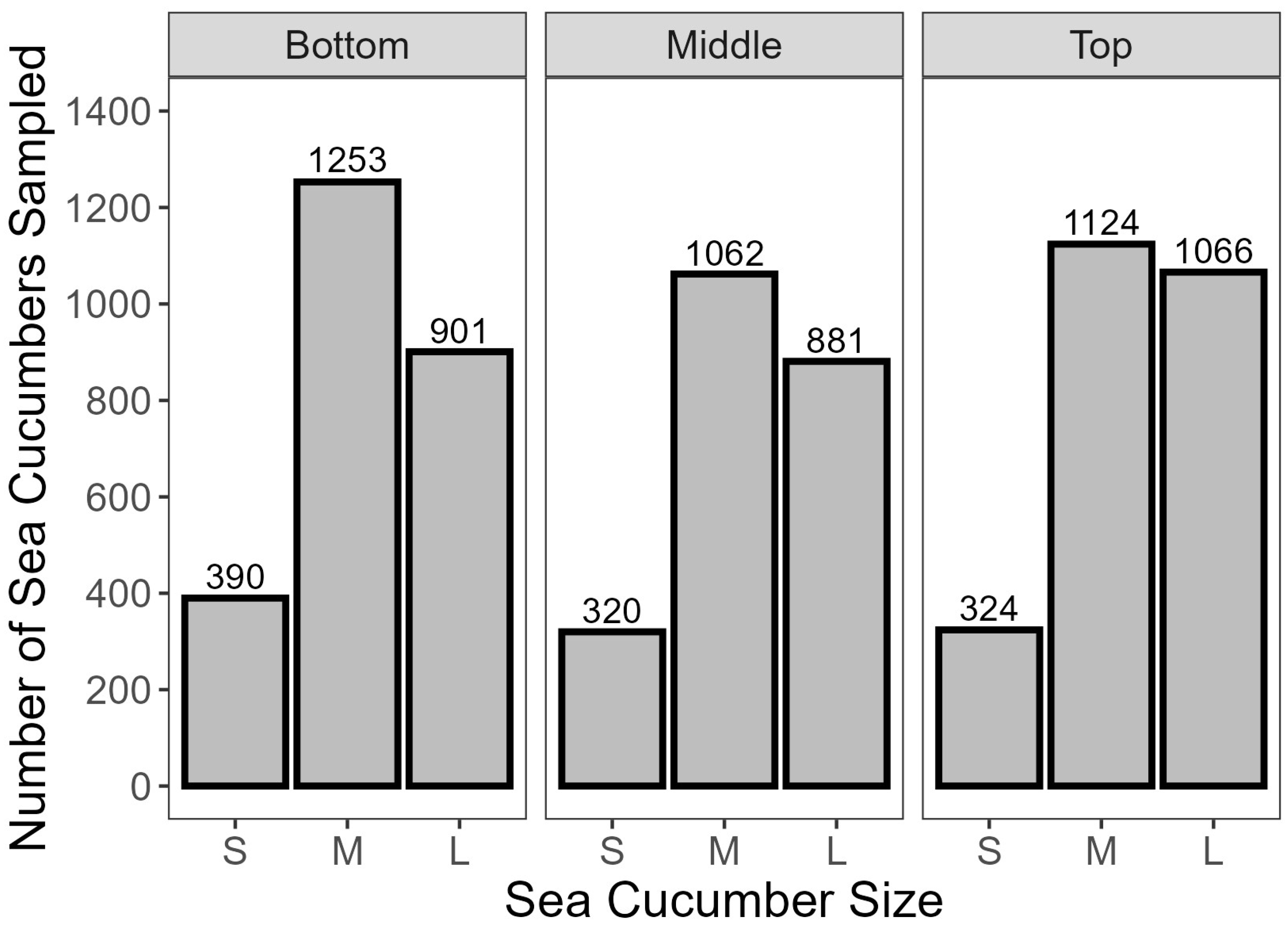
- In total, 18 pans were collected, six from each of the bottom, middle and top of the hold.
- The remaining product in each tote was returned for processing.
2.1.2. Subsample Collection for Evaluation
- The Ohaus and Western scales were tared for the weight of the bus pans and the Transcell scale was tared for the weight of the StackNest pans.
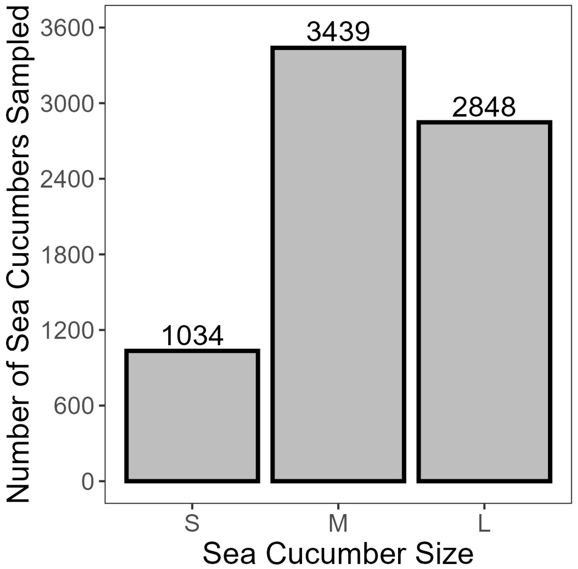
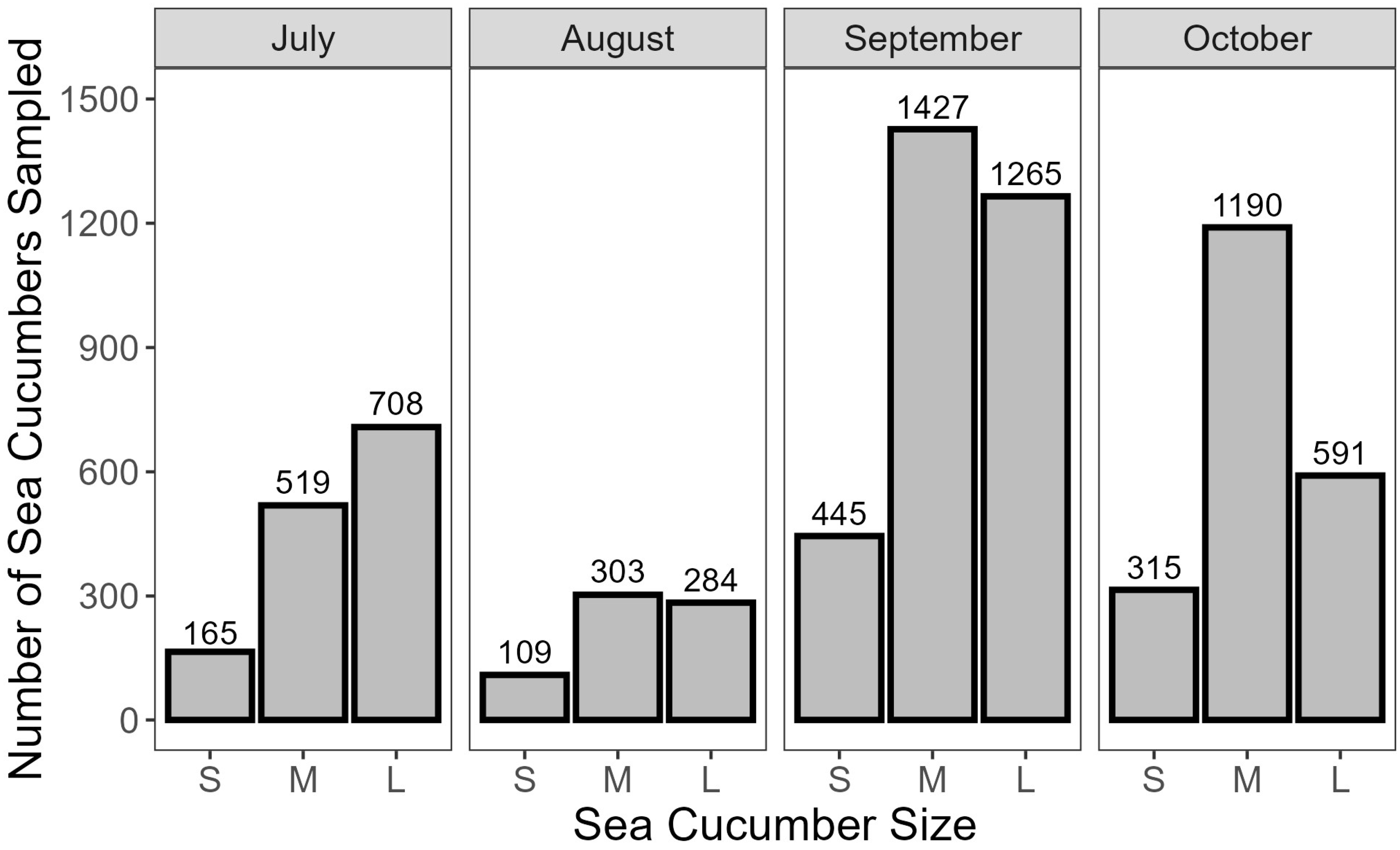
- Beginning with the six StackNest pans collected from the top layer, sea cucumbers were randomly selected one at a time from each StackNest pan, weighed, and sorted based on landed round weight (x ≤ 150 g = small, 150 < x ≤ 250 g = medium, and x > 250 g = large). These size bands were selected based on the range of available animal sizes and were used throughout the project.
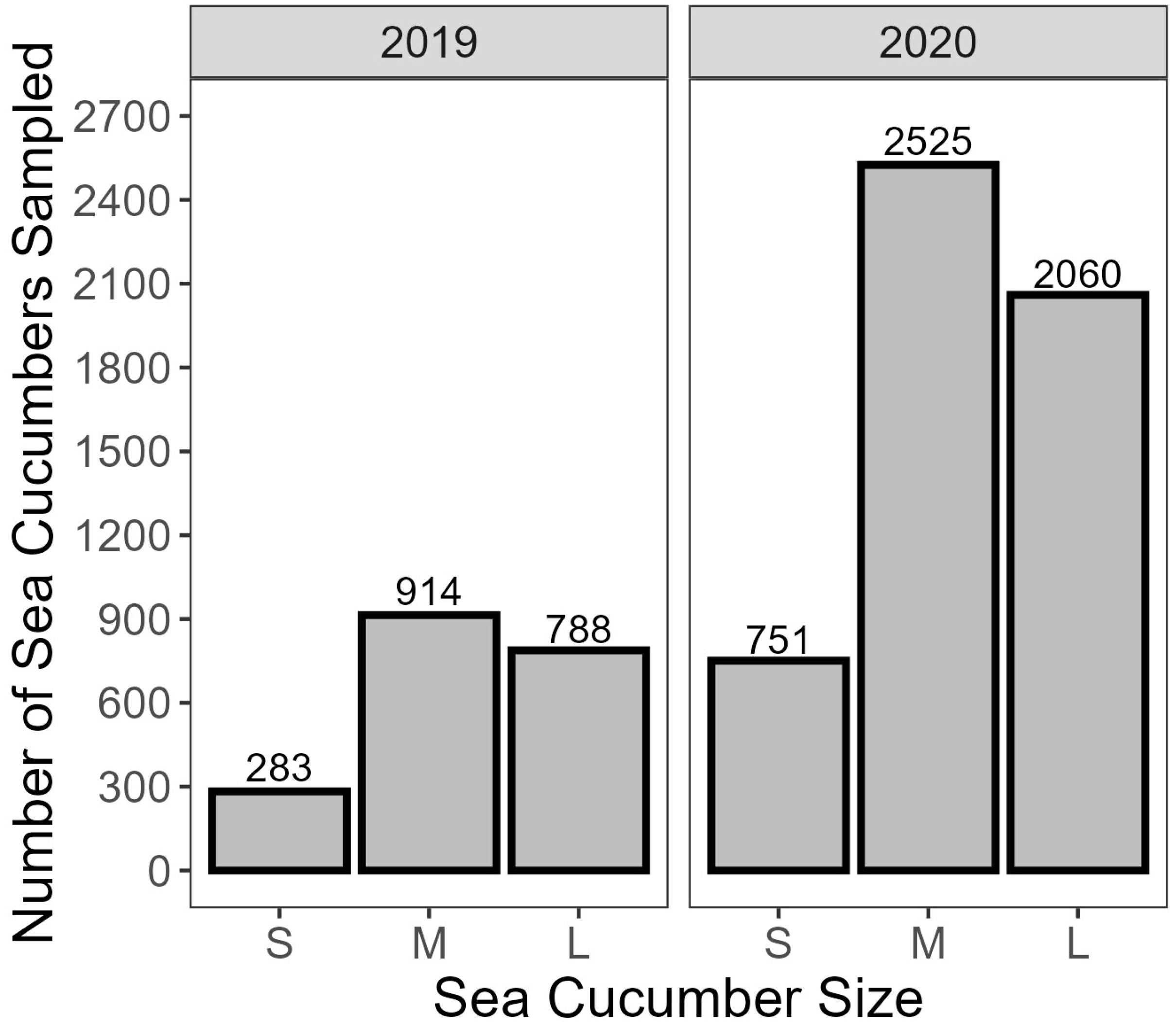
- An amount of 12 sea cucumbers, 40 each of small, medium and large size, were collected from each layer for water loss testing.
- The sampling time, net weight of the sample, and sample weighing time (to estimate the time duration between sampling and weighing) were recorded on the data collection form (Supplementary Materials).
- Once sufficient samples were collected, the expelled water remaining in the StackNest pan was weighed and recorded on the data collection form.
- Each bus pan was tagged with the size, location, and time the sample was collected.
- Approximately 230 random individuals were weighed for each of the top, middle, and bottom layers at each landing to estimate a size distribution for the project.
- The remaining sea cucumbers were returned to the processor for processing.
- This procedure was repeated for the middle and bottom layers of sea cucumber.
2.1.3. Quantifying Water Loss in Samples
- The Ohaus and Western scales were tared for the weight of the bus pans.
- Beginning with the small sea cucumbers collected from the top layer of the hold, we undertook the following:
- A set of five animals was selected at random.
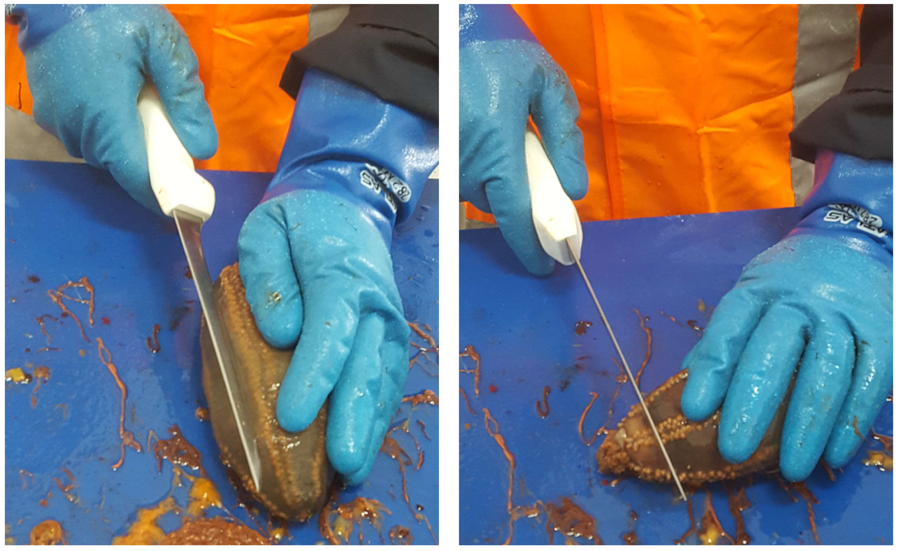
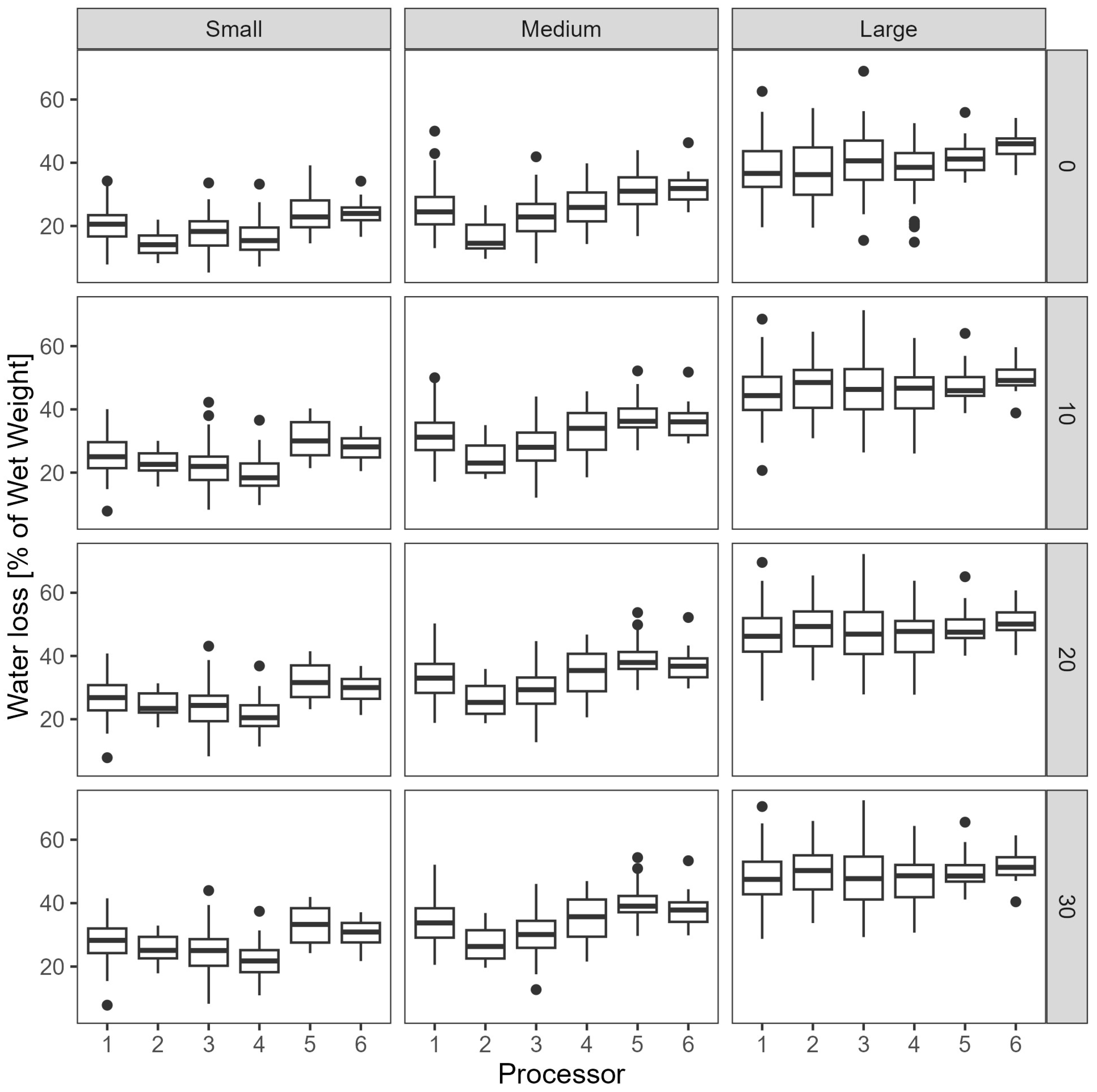
- Two sets were taken at a time, one for the longitudinal cut and one for the flower cut (Figure 2).
- Each set of five individuals was weighed and the weight recorded.
- Each individual was cut, the water sack broken, and placed back in the bus pan.
- In the case of flower cut samples, the trimmings were saved.
- To calculate the initial water loss, each set of five animals was weighed again immediately after cutting and the weight recorded.
- In the case of flower cut samples, the trimmings were weighed for each set and the weight was recorded.
- Each set was placed on the lump roe drain screen to drain.
- Steps 1–6 were repeated for each set of five individuals in the sample group (e.g., top layer, small animals).
- The water remaining in the bus pan was weighed and recorded.
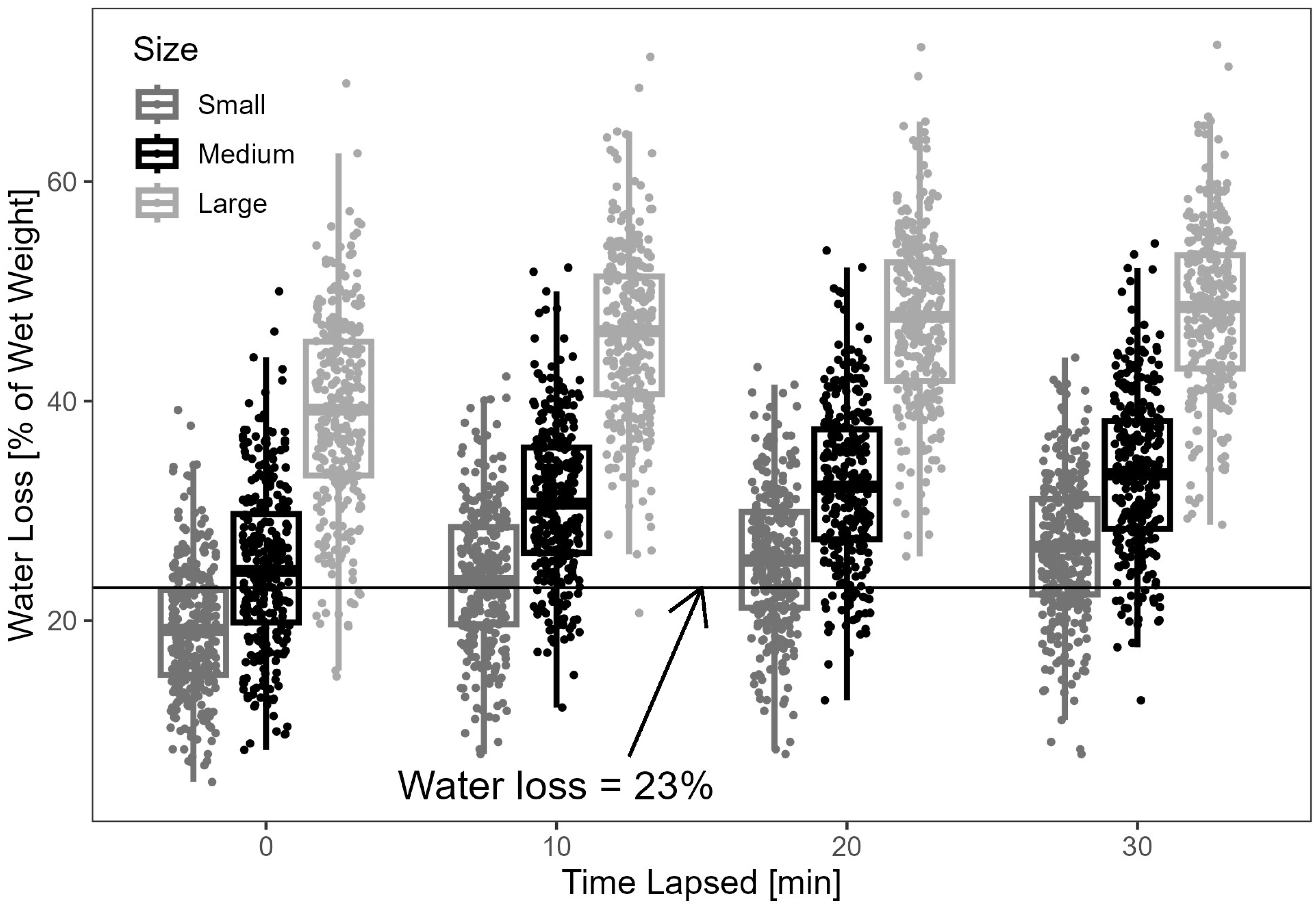
- The weight of each of the eight sample sets was measured after draining for 10, 20 and 30 min and recorded.
- This procedure was repeated for each of the nine sample groups.
2.2. Data Analysis
2.3. Trim Loss
2.4. Total Water Loss for Each Sample
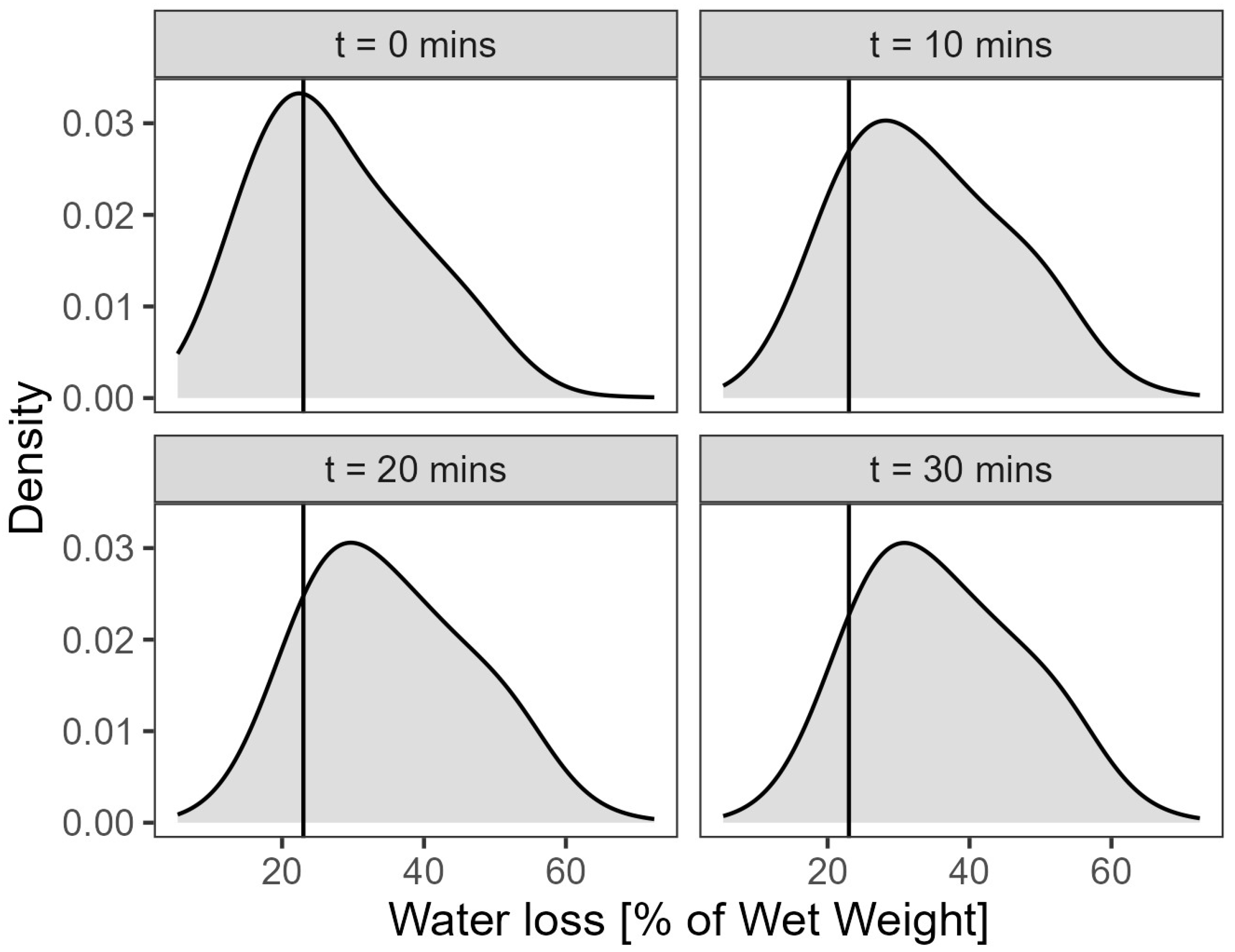
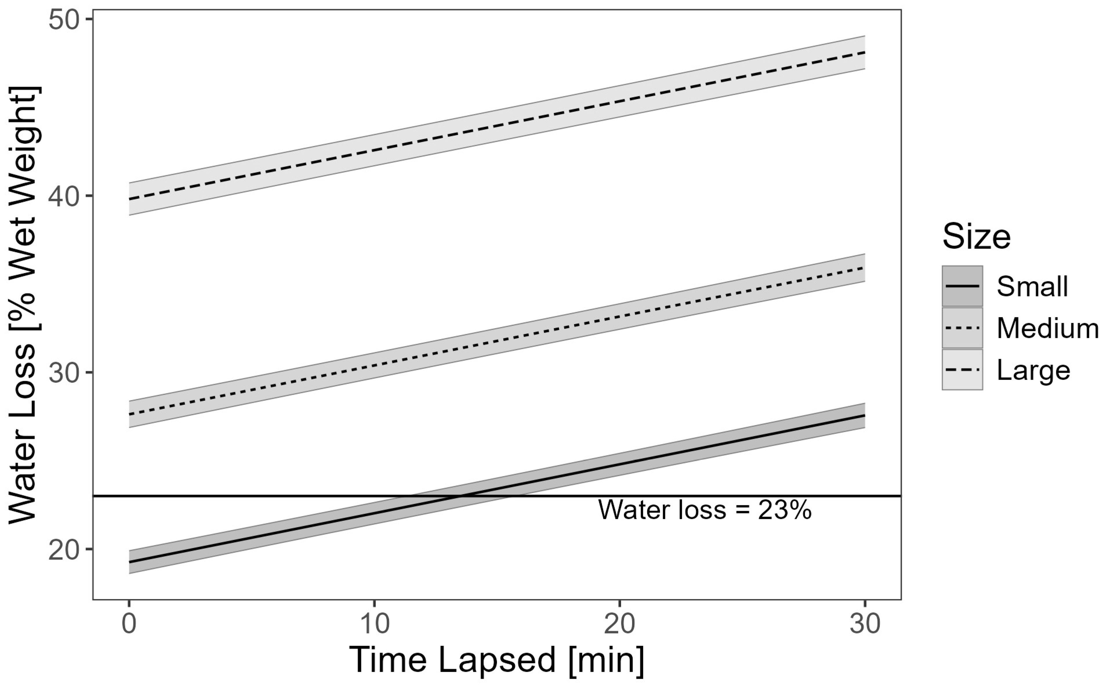
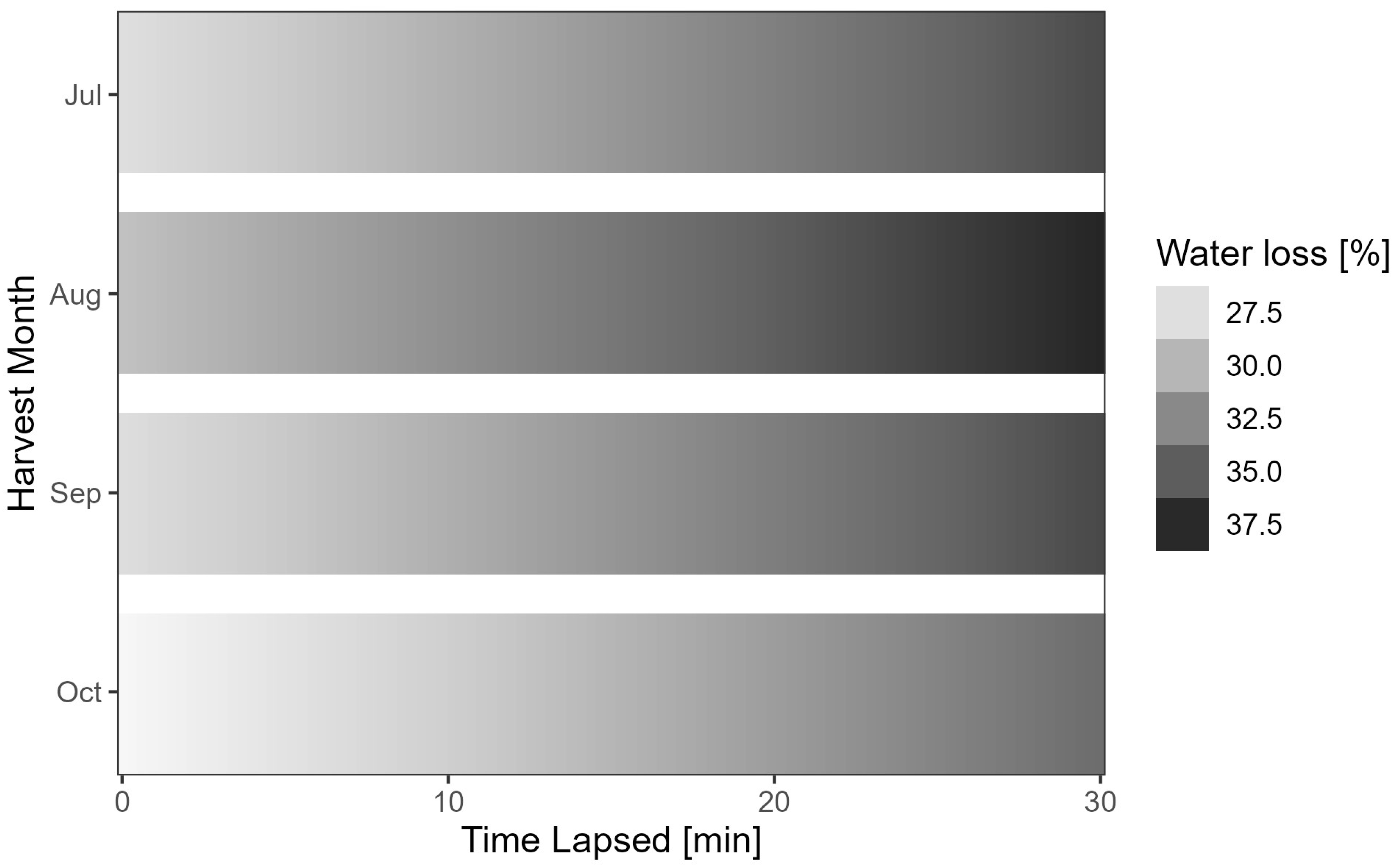
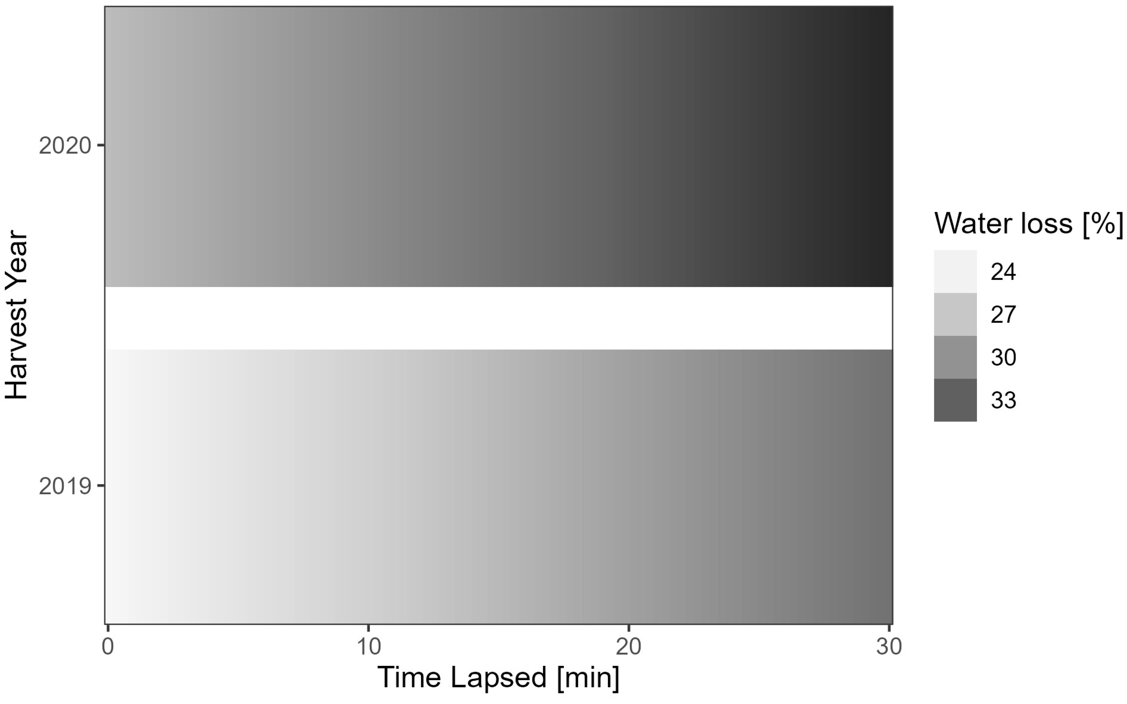
3. Results
3.1. Preliminary Water Loss Analysis
3.2. Statistical Analysis
E = µi = κi θi
σ2i = κi θ2i
4. Discussion
5. Conclusions
Supplementary Materials
Author Contributions
Funding
Institutional Review Board Statement
Informed Consent Statement
Data Availability Statement
Acknowledgments
Conflicts of Interest
Abbreviations
| BIC | Bayesian information criteria |
| DFO | Fisheries and Oceans Canada |
| EEZ | Exclusive economic zone |
| GADM | Global administrative areas |
| NAFO | North Atlantic Fisheries Organization |
| SPM | St. Pierre and Miquelon |
Appendix A
Appendix A.1. Equipment
- Western Scale digital indicator (#M2000, Western Scale Co., Ltd., Port Coquitlam, BC, Canada) with a TSS 16″ × 16″ stainless steel base (#TSS1616, The Scale Shop, St. John’s, NL, Canada).
- This scale has a 25 kg capacity and a 0.005 kg resolution.
- This scale’s calibration was certified in January 2019 and January 2020.
- The calibration was checked periodically throughout each sampling season.
- Ohaus Defender 5000 scale with digital indicator (#D52XW25WQR5, Ohaus Corp., Parsippany, NJ, USA).
- This scale has a 25 kg capacity with a 0.001 kg resolution.
- The scale’s calibration was certified in December 2019 and July 2020.
- The calibration was checked periodically throughout the 2020 sampling season.
- Transcell digital indicator and 16″ × 16″ stainless steel base (#TI-500E SS, Transcell Technologies Inc., Buffalo Grove, IL, USA).
- This scale has a 50 kg capacity and a 0.01 kg resolution.
- This scale was certified in January 2019 and July 2020.
- The calibration was checked periodically throughout each sampling season.
- Seventy-liter StackNest closed pans (#60258 70L, IPL Inc., St-Damien de Buckland, QC, Canada).
- Fourteen-liter Rubbermaid commercial bus pans (#FG334992GRAY, Newell Brands Co., Atlanta, GA, USA).
- Vented drying pans (#11020, Sommer-Allibert S.A., La Défense, France).
- Lump roe drain screens (#43186, C&W Industrial Fabrication & Marine Equipment, Bay Bulls, NL, Canada).
- Insulated totes with capacities of 1000 and 2000 L (various brands, processor supplied).
- Additional items included filleting knives, and Teflon tags.
References
- Yang, H.; Bai, Y. Apostichopus japonicus in the life of Chinese people. In Developments in Aquaculture and Fisheries Science, 1st ed.; Yang, H., Hamel, J.-F., Mercier, A., Eds.; Academic Press: London, UK, 2015; Volume 39, pp. 1–23. [Google Scholar]
- Hossain, A.; Dave, D.; Shahidi, F. Northern sea cucumber (Cucumaria frondosa): A potential candidate for functional food, nutraceutical, and pharmaceutical sector. Mar. Drugs 2020, 18, 274. [Google Scholar] [CrossRef] [PubMed]
- Bordbar, S.; Anwar, F.; Saari, N. High-value components and bioactives from sea cucumbers for functional foods—A review. Mar. Drugs 2011, 9, 1761–1805. [Google Scholar] [CrossRef] [PubMed]
- Gianasi, B.L.; Hamel, J.-F.; Montgomery, E.M.; Sun, J.; Mercier, A. Current knowledge on the biology, ecology, and commercial exploitation of the sea cucumber Cucumaria frondosa. Rev. Fish. Sci. Aquac. 2021, 29, 582–653. [Google Scholar] [CrossRef]
- Purcell, S.W.; Lovatelli, A.; Vasconcellos, M.; Ye, Y. Managing Sea Cucumber Fisheries with an Ecosystem Approach; Food and Agriculture Organization of the United Nations: Rome, Italy, 2010. [Google Scholar]
- Purcell, S.W.; Mercier, A.; Conand, C.; Hamel, J.F.; Toral-Granda, M.V.; Lovatelli, A.; Uthicke, S. Sea cucumber fisheries: Global analysis of stocks, management measures and drivers of overfishing. Fish Fish. 2013, 14, 34–59. [Google Scholar] [CrossRef]
- So, J.J.; Hamel, J.-F.; Mercier, A. Habitat utilisation, growth and predation of Cucumaria frondosa: Implications for an emerging sea cucumber fishery. Fish. Manag. Ecol. 2010, 17, 473–484. [Google Scholar] [CrossRef]
- Anderson, S.C.; Flemming, J.M.; Watson, R.; Lotze, H.K. Serial exploitation of global sea cucumber fisheries. Fish Fish. 2011, 12, 317–339. [Google Scholar] [CrossRef]
- Fisheries and Oceans Canada. Sea Cucumber Newfoundland and Labrador Region 3Ps. Available online: https://www.dfo-mpo.gc.ca/fisheries-peches/ifmp-gmp/sea_cucumber-holothuries/2019/index-eng.html (accessed on 20 May 2022).
- Nelson, E.J.; MacDonald, B.A.; Robinson, S.M.C. A review of the Northern sea cucumber Cucumaria frondosa (Gunnerus, 1767) as a potential aquaculture species. Rev. Fish. Sci. 2012, 20, 212–219. [Google Scholar] [CrossRef]
- Department of Fisheries Forestry and Agriculture. Seafood Industry Year in Review 2023. Available online: https://www.gov.nl.ca/ffa/files/Seafood-Industry-Year-in-Review-2023.pdf (accessed on 3 February 2025).
- Wickham, H. ggplot2: Elegant Graphics for Data Analysis; Springer: New York, NY, USA, 2016. [Google Scholar]
- Lampbert, P. Sea Cucumbers of British Columbia, Southeast Alaska and Puget Sound; UBC Press: Vancouver, BC, Canada, 1997. [Google Scholar]
- Hamel, J.F.; Sun, J.; Gianasi, B.L.; Montgomery, E.M.; Kenchington, E.L.; Burel, B.; Rowe, S.; Winger, P.D.; Mercier, A. Active buoyancy adjustment increases dispersal potential in benthic marine animals. J. Anim. Ecol. 2019, 88, 820–832. [Google Scholar] [CrossRef] [PubMed]
- Skewes, T.; Smith, L.; Dennis, D.; Rawlinson, N.; Donovan, A.; Ellis, N. Conversion Ratios for Commercial Beche-de-mer Species in Torres Strait; CISRO Marine Research: Canberra, Australia, 2004; p. 32. [Google Scholar]
- Grant, S.M.; Squire, L.; Keats, C. Biological Resource Assessment of the Orange Footed Sea Cucumber (Cucumaria frondosa) Occurring on the St. Pierre Bank; Centre for Sustainable Aquatic Resources, Fisheries and Marine Institute of the Memorial University of Newfoundland: St. John’s, NL, Canada, 2006. [Google Scholar]
- Gianasi, B.L.; Hamel, J.-F.; Mercier, A. Experimental test of optimal holding conditions for live transport of temperate sea cucumbers. Fish. Res. 2016, 174, 298–308. [Google Scholar] [CrossRef]
- Trenholm, R.G.; Montgomery, E.M.; Hamel, J.-F.; Rowe, S.; Gianasi, B.L.; Mercier, A. Exploring body-size metrics in sea cucumbers through a literature review and case study of the commercial dendrochirotid Cucumaria frondosa. In The World of Sea Cucumbers: Challenges, Advances, and Innovations; Mercier, A., Hamel, J.-F., Suhrbier, A.D., Pearce, C.M., Eds.; Academic Press: London, UK, 2024; pp. 521–546. [Google Scholar]
- Department of Fisheries Forestry and Agriculture. Standing Fish Price-Setting Panel: Sea Cucumber Fishery-2022. Available online: https://www.gov.nl.ca/fishpanel/pricingdecisions/2022/Sea-Cucumber-Fishery-Decision-May-18.pdf (accessed on 30 May 2022).
- Ortola, M.L. Number Generator Random, 2.1; Apple: Cupertino, CA, USA, 2018. [Google Scholar]
- Zuur, A.F.; Ieno, E.N. A protocol for conducting and presenting results of regression-type analyses. Methods Ecol. Evol. 2016, 7, 636–645. [Google Scholar] [CrossRef]
- R Core Team. R: A Language and Environment for Statistical Computing; R Foundation for Statistical Computing: Vienna, Austria, 2022. [Google Scholar]
- Wickham, H.; Averick, M.; Bryan, J.; Chang, W.; D’Agostino McGowan, L.; François, R.; Grolemund, G.; Hayes, A.; Henry, L.; Hester, J.; et al. Welcome to the tidyverse. J. Open Source Softw. 2019, 4, 1686. [Google Scholar] [CrossRef]
- Grolemund, G.; Wickham, H. Dates and times made easy with lubridate. J. Stat. Softw. 2011, 40, 1–25. [Google Scholar] [CrossRef]
- Dunn, P.K.; Smyth, G.K. Randomized quantile residuals. J. Comput. Graph. Stat. 1996, 5, 236–244. [Google Scholar] [CrossRef]
- Venables, W.N.; Ripley, B.D. Modern Applied Statistics with S, 4th ed.; Springer: New York, NY, USA, 2002. [Google Scholar]
- Zuur, A.F.; Ieno, E.N.; Elphick, C.S. A protocol for data exploration to avoid common statistical problems. Methods Ecol. Evol. 2010, 1, 3–14. [Google Scholar] [CrossRef]
- Fox, J. Applied Regression Analysis and Generalized Linear Models, 2nd ed.; Sage Publications Ltd.: Thousand Oaks, CA, USA, 2008. [Google Scholar]
- Dunn, P.K.; Smyth, G.K. Positive continuous data: Gamma and Inverse Gaussian GLMs. In Generalized Linear Models with Examples in R; DeVeaux, R., Fienberg, S.E., Olkin, I., Eds.; Springer: New York, NY, USA, 2018; pp. 425–456. [Google Scholar]
- Das, B.K.; Jha, D.N.; Sahu, S.K.; Yadav, A.K.; Raman, R.K.; Kartikeyan, M. Chi-Square Test of Significance. In Concept Building in Fisheries Data Analysis; Springer Nature: Singapore, 2023; pp. 81–94. [Google Scholar]
- Schwarz, G. Estimating the dimension of a model. Ann. Stat. 1978, 6, 461–464. [Google Scholar] [CrossRef]
- Breheny, P.; Burchett, W. Visualization of regression models using visreg. R J. 2017, 9, 56–71. [Google Scholar] [CrossRef]
- Fish Food & Allied Workers. Sea Cucumber Price–2023. Available online: https://ffaw.ca/our-fish-prices/sea-cucumber-price-2023/ (accessed on 22 June 2023).
- Batt, J.; Bennett-Steward, K.; Couturier, C.; Hammell, L.; Harvey-Clark, C.; Krieiberg, H.; Iwama, G.; Lall, S.; Litvak, M.; Rainnie, D.; et al. CCAC Guidelines on the Care and Use of Fish in Research, Teaching, and Testing; Canadian Council on Animal Care: Ottawa, ON, Canada, 2005; p. 85. [Google Scholar]


| Date | Offloading Location | Fishing Area | Hail Weight (lbs.) 1 | Offloading Method |
|---|---|---|---|---|
| 22 August 2019 | OCI, St. Lawrence | Western Bank | 60,000 | Vacuum |
| 30 August 2019 | OCI, St. Lawrence | Eastern Bank | 90,000 | Vacuum |
| 21 September 2019 | QuinSea, Fortune | Western Bank | 50,000 | Bucket |
| 27 September 2019 | OCI, Fortune | Eastern Bank | 90,000 | Bucket |
| 11 October 2019 | OCI, St. Lawrence | Eastern Bank | 55,000 | Vacuum |
| 22 July 2020 | OCI, St. Lawrence | Eastern Bank | 63,000 | Vacuum |
| 29 July 2020 | QuinSea, Fortune | Western Bank | 96,000 | Bucket |
| 11 August 2020 | QuinSea, Fortune | Western Bank | 95,000 | Bucket |
| 3 September 2020 | Clearwater Grand Bank | Eastern Bank | 45,000 | Vacuum |
| 17 September 2020 | Green, Burin | Western Bank | 55,000 | Vacuum |
| 29 September 2020 | Fogo, Riverhead | Eastern Bank | 60,000 | Vacuum |
| 7 October 2020 | Clearwater Grand Bank | Eastern Bank | 60,000 | Vacuum |
| 14 October 2020 | OCI, St. Lawrence | Eastern Bank | 33,000 | Vacuum |
| Description | 2019 | 2020 |
|---|---|---|
| Trips | 5 | 8 |
| Hold locations | 3 | 3 |
| Sea cucumber sizes | 3 | 3 |
| Cut methods | 2 | 2 |
| Sets | 4 | 4 |
| Water loss times | 4 | 4 |
| Total data points | 1440 | 2200 1 |
| Variable | Type | Levels | Units | Values |
|---|---|---|---|---|
| License (L) | Factor | 12 | AB, AP, AS, BG, CY, DM, HM, JC, KA, PS, TK, WS | |
| Processor (P) | Factor | 6 | 1, 2, 3, 4, 5, 6 | |
| Bank (B) | Factor | 2 | Eastern, Western | |
| Transfer (T) | Factor | 2 | Bucket, vacuum transfer | |
| Month (M) | Factor | 4 | Oct, Sept, Aug, Jul | |
| Year (Y) | Factor | 2 | 2019, 2020 | |
| Location (L) | Factor | 3 | Bottom, middle, top | |
| Size (S) | Factor | 3 | Small, medium, large | |
| Cut (C) | Factor | 2 | Flower, longitudinal | |
| Lapsed (t) | Integer | mins | 10, 20, 30, 40 | |
| TLapsed (tl) | Integer | mins | 84–661 | |
| Free water (FW) | Number | kg | 0.034–2.786 | |
| Free water % (FWp) | Number | % | 5.28–72.46 |
| Df | Deviance | Scaled Dev | p (>Chi) | |
|---|---|---|---|---|
| <none> | 176.81 | |||
| Lapsed | 1 | 214.50 | 833.34 | <2.2 × 10⁻¹⁶ |
| Mon | 3 | 182.50 | 125.93 | <2.2 × 10⁻¹⁶ |
| Location | 2 | 190.69 | 306.97 | <2.2 × 10⁻¹⁶ |
| Cut | 1 | 178.66 | 41.12 | 1.43 × 10⁻¹⁰ |
| Size:Transfer | 2 | 180.88 | 90.11 | <2.2 × 10⁻¹⁶ |
| Size:Year | 2 | 178.88 | 45.75 | 1.16 × 10⁻¹⁰ |
| Estimate | Std. Error | t | p (>|t|) | |
|---|---|---|---|---|
| (Intercept) | 12.936 | 0.422 | 30.669 | <2 × 10⁻¹⁶ |
| Lapsed | 0.277 | 0.009 | 30.010 | <2 × 10⁻¹⁶ |
| Size = medium (M) | 2.980 | 0.405 | 7.364 | 2.19 × 10⁻¹³ |
| Size = large (L) | 23.201 | 0.614 | 37.802 | <2 × 10⁻¹⁶ |
| Mon = Sep | 1.778 | 0.295 | 6.019 | 1.93 × 10−09 |
| Mon = Aug | 3.538 | 0.318 | 11.120 | <2 × 10⁻¹⁶ |
| Mon = Jul | 1.687 | 0.377 | 4.477 | 7.82 × 10−06 |
| Year = 2020 | 0.883 | 0.306 | 2.882 | 3.98 × 10−03 |
| Location = middle | 0.149 | 0.296 | 0.624 | 0.533 |
| Location = top | 3.927 | 0.255 | 15.421 | <2 × 10⁻¹⁶ |
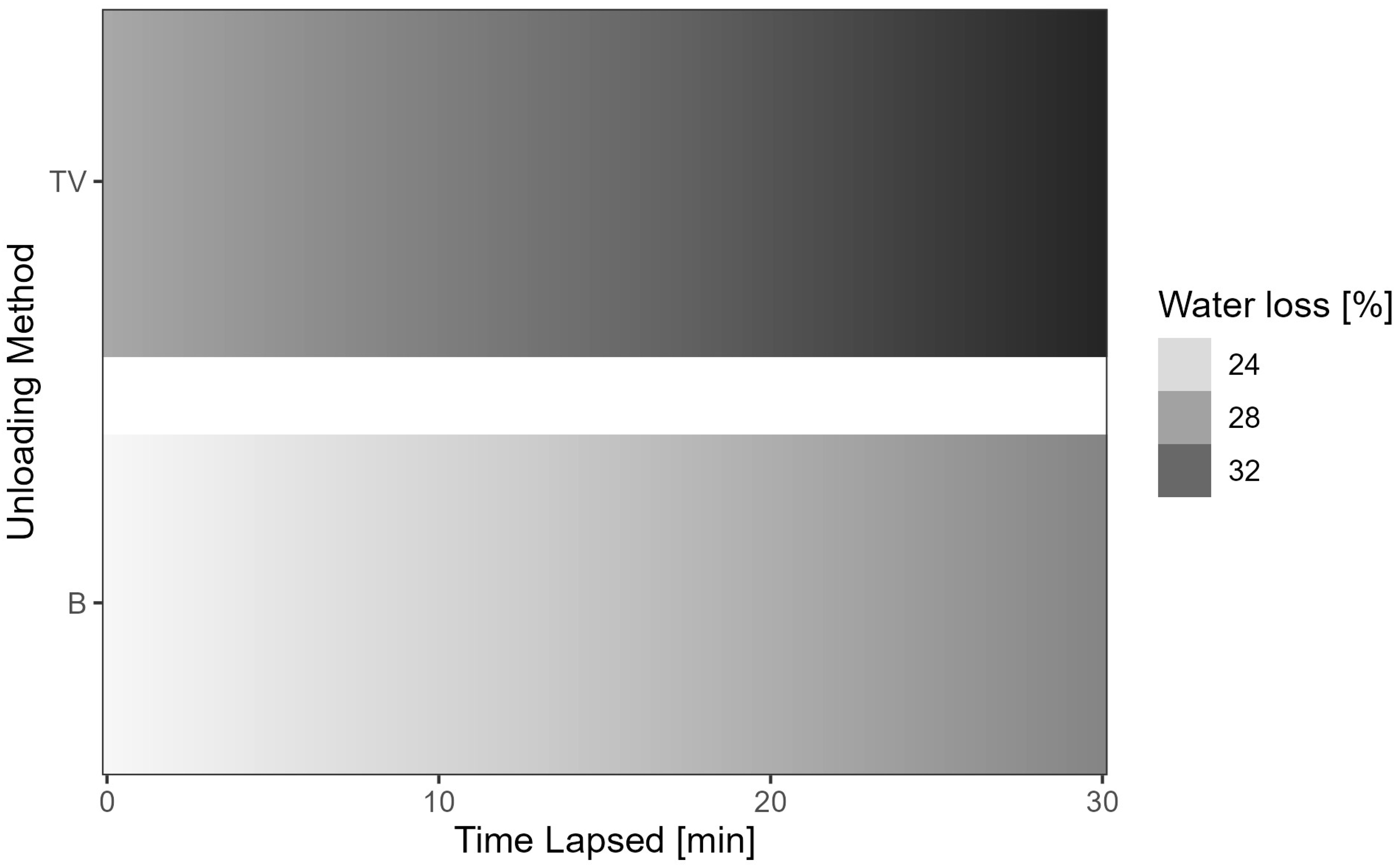
| Transfer = vacuum (TV) | 3.662 | 0.316 | 11.603 | <2 × 10⁻¹⁶ |
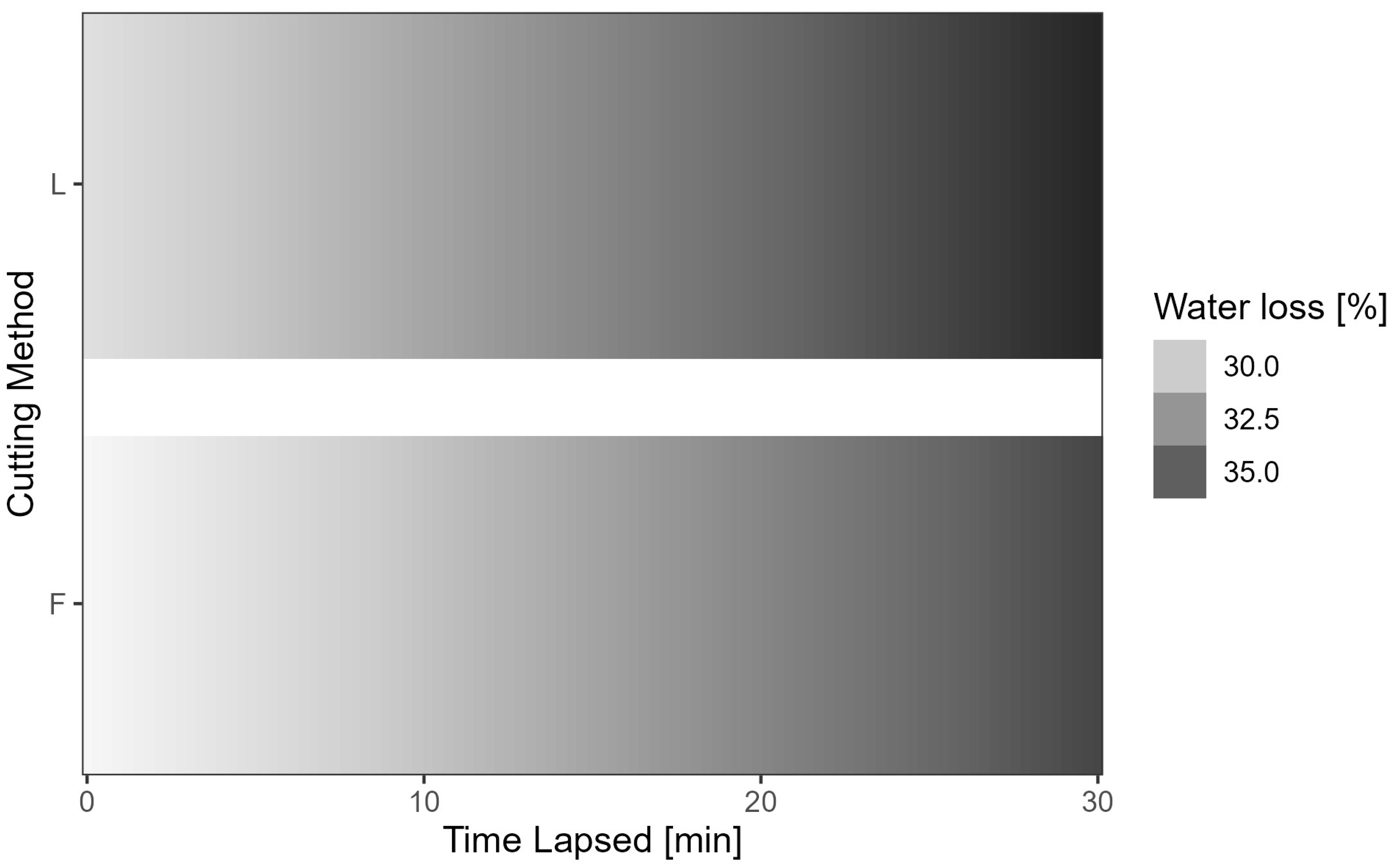
| Cut = longitudinal | 1.311 | 0.203 | 6.445 | 1.31 × 10⁻¹⁰ |
| Size = M × transfer = TV | 2.287 | 0.468 | 4.886 | 1.07 × 10−06 |
| Size = L × transfer = TV | −4.257 | 0.666 | −6.395 | 1.81 × 10⁻¹⁰ |
| Size = M × year = 2020 | 3.098 | 0.462 | 6.710 | 2.25 × 10⁻¹¹ |
| Size = L × year = 2020 | 1.604 | 0.631 | 2.542 | 0.011 |
| 2.5% | 97.5% | |
|---|---|---|
| (Intercept) | 12.111 | 13.771 |
| Lapsed | 0.258 | 0.296 |
| Size = medium (M) | 2.176 | 3.789 |
| Size = large (L) | 22.008 | 24.415 |
| Mon = Sep | 1.200 | 2.355 |
| Mon = Aug | 2.916 | 4.160 |
| Mon = Jul | 0.946 | 2.432 |
| Year = 2020 | 0.284 | 1.481 |
| Location = middle | −0.322 | 0.621 |
| Location = top | 3.428 | 4.427 |
| Transfer = vacuum (TV) | 3.040 | 4.428 |
| Cut = longitudinal | 0.910 | 1.713 |
| Size = M × transfer = TV | 1.372 | 3.201 |
| Size = L × transfer = TV | −5.569 | −2.956 |
| Size = M × year = 2020 | 2.197 | 4.000 |
| Size = L × year = 2020 | 0.364 | 2.840 |
Disclaimer/Publisher’s Note: The statements, opinions and data contained in all publications are solely those of the individual author(s) and contributor(s) and not of MDPI and/or the editor(s). MDPI and/or the editor(s) disclaim responsibility for any injury to people or property resulting from any ideas, methods, instructions or products referred to in the content. |
© 2025 by the authors. Licensee MDPI, Basel, Switzerland. This article is an open access article distributed under the terms and conditions of the Creative Commons Attribution (CC BY) license (https://creativecommons.org/licenses/by/4.0/).
Share and Cite
Brown, P.; Burke, H.J.; Goyali, J.C.; Murphy, W.; Dave, D. Seasonal Trends in Water Retention of Atlantic Sea Cucumber (Cucumaria frondosa): A Modeling Approach. Fishes 2025, 10, 212. https://doi.org/10.3390/fishes10050212
Brown P, Burke HJ, Goyali JC, Murphy W, Dave D. Seasonal Trends in Water Retention of Atlantic Sea Cucumber (Cucumaria frondosa): A Modeling Approach. Fishes. 2025; 10(5):212. https://doi.org/10.3390/fishes10050212
Chicago/Turabian StyleBrown, Pete, Heather J. Burke, Juran C. Goyali, Wade Murphy, and Deepika Dave. 2025. "Seasonal Trends in Water Retention of Atlantic Sea Cucumber (Cucumaria frondosa): A Modeling Approach" Fishes 10, no. 5: 212. https://doi.org/10.3390/fishes10050212
APA StyleBrown, P., Burke, H. J., Goyali, J. C., Murphy, W., & Dave, D. (2025). Seasonal Trends in Water Retention of Atlantic Sea Cucumber (Cucumaria frondosa): A Modeling Approach. Fishes, 10(5), 212. https://doi.org/10.3390/fishes10050212