Effects of Sampling Design on Population Abundance Estimation of Ichthyoplankton in Coastal Waters

Abstract

The abundance, spatial distribution of and dynamic changes in ichthyoplankton species affect the recruitment and fish population dynamics, which are fundamental for stock assessment and fisheries management. An evaluation of alternative sampling designs needs to be carried out to determine the optimal scheme that is cost-effective in collecting high-quality ichthyoplankton data. A simulation study was conducted to evaluate the performances and consistency of six potential sampling designs for an ichthyoplankton survey in the coastal waters of the central and southern Yellow Sea. Relative estimation error (REE) and relative bias (RB) were used to measure the performances in estimating the population abundances of five target ichthyoplankton species in different sampling designs. In general, the two systematic sampling (SYS) designs had high precision and accuracy estimation and remained stable over years for estimating the population abundance of ichthyoplankton species compared with the other four sampling designs. SYS did not result in the overestimation or underestimation of the mean population abundance. Most sampling designs showed relatively high accuracy in abundance estimation when sample sizes were higher than medium levels. This study could improve the performances of sampling designs of ichthyoplankton surveys and provide a reference for the further optimization of sampling designs.

1. Introduction

Fishery-independent surveys are fundamental in collecting data for assessment of fish population characteristics such as abundance and spatial distribution [1,2]. A well-designed fishery-independent survey can provide accurate information about population dynamics, which can be further used to make decisions for fishery management and the sustainable utilization of fishery resources [3]. With the increasing demand for high-quality data for fish stock assessment and management, sampling design and its optimization has attracted much attention [1,4,5,6,7,8].

Ichthyoplankton refers to the early life history stage of fishes, including eggs, larvae and juveniles. Ichthyoplankton monitoring programs are often conducted to collect information on the species composition, abundance, and geographical distribution of ichthyoplankton. Distribution patterns of ichthyoplankton influence their growth and survival rate, and habitat preference can lead to different spatiotemporal patterns [9,10,11]. The eggs and larvae of marine fishes are usually collected in fine-meshed plankton nets or specially designed gear [12]. Ichthyoplankton surveys can obtain data to estimate the distributions, abundance, diversity, and structure of ichthyoplankton communities, including associations of larvae with their predators and prey [13,14], which is usually a component of stock assessments and fisheries management. Monitoring ichthyoplankton abundance is also a relatively simple method to understand fish populations dynamics. The resulting ichthyoplankton data are often used in identifying fish stocks, inferring spawning locations and times, and estimating spawning stock biomass [15,16]. The abundance of, spatial distribution of, and changes in ichthyoplankton affect the early recruitment and dynamics of fish populations [17], which is important for fish stock assessment and management [18,19,20]. Many factors, such as environmental changes and human disturbances, may affect the traditional spawning environments of fish stocks, leading to changes in the spawning ground, abundance, and spatial distribution patterns of ichthyoplankton species over time [21,22].

Simple random sampling (SRS), stratified random sampling (StRS), fixed-station sampling (FS), cluster sampling (CS), and systematic sampling (SYS) are commonly used sampling designs in fishery-independent surveys. SRS is the simplest sampling design, and other complex sampling designs usually include SRS to some extent [23]. StRS divides the population into different stratum according to heterogeneities and conducts SRS at each stratum to improve the precision and accuracy of the estimation of population abundance [5,24,25,26]. FS is a repeated sampling at fixed stations, which can find different information at the same sampling station to compare the changes in resources over time [27,28,29]. CS has long history in ecology studies, and it is often adopted when environmental gradients are closely related to species distribution [4,30,31,32]. SYS is accurate when the target species is evenly and widely distributed [8,33]. The effects of sampling designs on the estimation of different survey objectives have been examined in many studies [8,25,26,27,34].

A well-designed sampling program is fundamental to high-quality data collection in ichthyoplankton surveys. Considering the various survey objectives, the accuracy and precision of estimation, and the cost saving, ichthyoplankton survey design has gradually attracted much attention. There have been some studies on ichthyoplankton sampling, involving sampling designs, gears, time series, sample sizes, and so on. Hernandez et al. [35] compared the effectiveness of two plankton mesh nets for an ichthyoplankton survey and found that these two nets were largely comparable. Pepin and Helbig [20] explored the influence of spatial scales and spatial sampling resolution on abundance estimate of ichthyoplankton. Koslow and Wright [36] examined the influence of the reduction in sampling time series or sample size on the abundance estimation of key species and patterns of community change. However, the evaluation and comparison of the performances of different sampling designs for choosing optimal designs are still relatively lacking. Fixed-station sampling designs and cluster sampling designs based on transects have been extensively applied in ichthyoplankton surveys [36,37,38,39]. Fixed-station surveys easily collect data over long time series and can guarantee the randomness of survey data due to the floating nature of ichthyoplankton itself [12]. Long et al. [40] compared different stratified sampling designs for two larvae species in the Yangtze Estuary and determined the optimal stratification scheme. The influences of sampling designs on the estimation of different characteristics of ichthyoplankton communities and the effectiveness of the survey designs need to be evaluated. Fishery-independent surveys are often expensive, and sampling procedures at sea are also often constrained by ocean conditions [41,42]. This requires an evaluation of alternative sampling designs to select a cost-effective scheme, which can allow us to obtain high-quality data with limited cost.

The objectives of this study are to evaluate the performances of different sampling designs and to find the optimal sampling design to improve the accuracy and precision of estimates of abundance indices for multiple ichthyoplankton species in the ichthyoplankton survey. This study could also provide a framework to evaluate the performances of sampling designs for multispecies ichthyoplankton surveys in coastal waters.

2. Materials and Methods

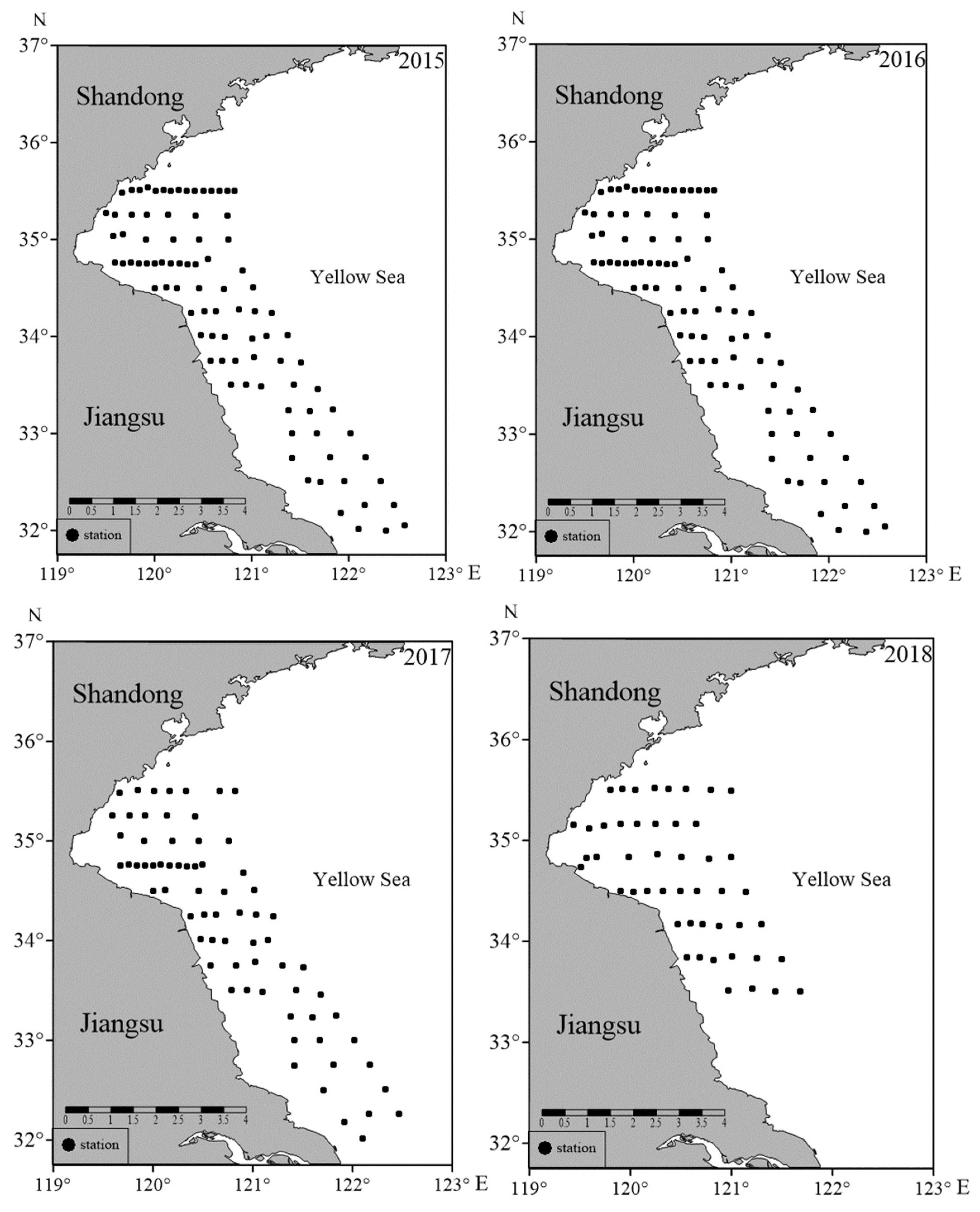
2.1. Data Collection

The coastal waters of the central and southern Yellow Sea are important spawning, feeding and nursery grounds for many fish species [43,44], and they are also traditional fishing grounds in China [45]. The spawning season is mainly from May to August, with a peak in June [43].

The ichthyoplankton surveys were conducted to collect information on the overall species composition and abundance indices of ichthyoplankton species in June from 2015 to 2018 in the coastal waters of the central and southern Yellow Sea. The survey area ranged from 32° N to 35.5° N and from 119° E to 123° E. The number of survey stations was set at 90, 89, 72, and 48 from 2015 to 2018, respectively (Figure 1). The ichthyoplankton surveys were conducted using a large horizontal trawl net, with the towing speed being about 2 knots and the hauling duration being 10 min on average at each survey station. A single general oceanic flowmeter mounted at the mouth of the nets was used to estimate the volume of water filtered. The length and mouth diameter of the sampling net were 2.8 m and 0.8 m respectively, and the mesh size was 0.505 mm.

The ichthyoplankton samples were preserved in 5% sea water formalin neutral solution. The collection and preservation of ichthyoplankton samples were conducted according to the Specifications for Oceanographic Survey Part 6: Marine Biological Survey (GB/T12763.6-2007) [46]. All ichthyoplankton were subsequently separated from other planktonic organisms and identified by species or to the lowest taxonomic level possible. Eggs, larvae, and juveniles were observed with laboratory microscopy, and species identification was carried out with reference to Fish Eggs and Larvae in China Seas [47] and Eggs and Larvae of Fish in the Coastal and Adjacent Waters of China [48].

2.2. ‘True’ Values Based on Ordinary Kriging Interpolation

Red tonguesole (Cynoglossus joyneri, CJ), silver sillago (Sillago sihama, SS), Commerson’s anchovy (Stolephorus commersonni, SC), dragonet (Callionymus·spp., CM), and Japanese anchovy (Engraulis japonicus, EJ) were chosen as the target species in the ichthyoplankton surveys in this study.

The sampling unit size of the interpolated abundance maps was 3′ × 3′, and there were 3661 potential sampling units in the surveyed waters. Ordinary kriging interpolation (OKI) was used to interpolate the relative abundance data at un-surveyed locations by combing weights and values at surveyed locations for the target ichthyoplankton species from 2015 to 2018, respectively [49]. The weights were estimated according to semi-variance among known values [50,51]. We assumed that the current survey design could represent the ‘true’ spatial distribution of ichthyoplankton species in the study area, and the interpolated relative abundance data based on OKI were regarded as the ‘true’ values for each species in each sampling unit in this simulation study.

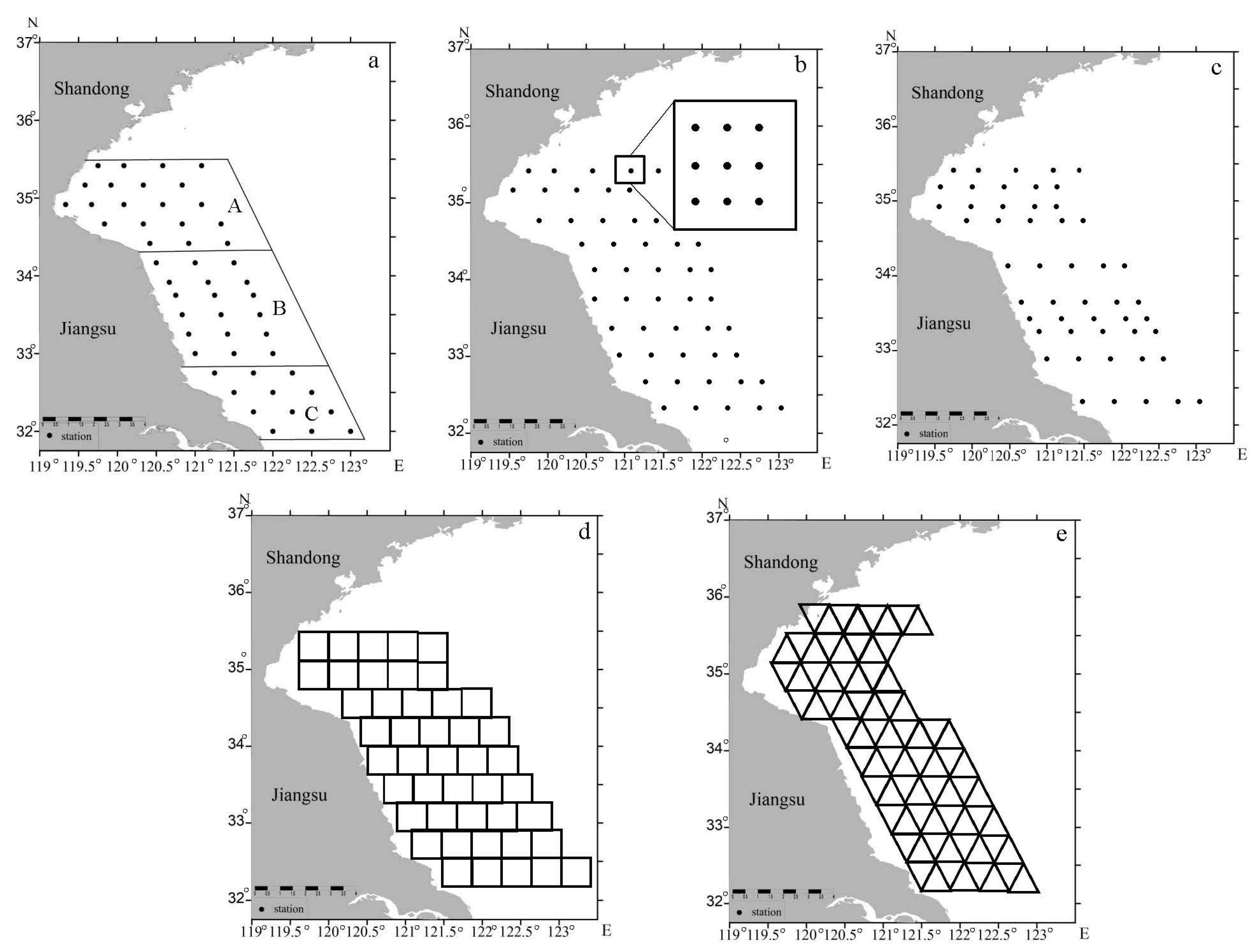
2.3. Sampling Designs

Six sampling methods and four levels of sample size were considered in the following potential sampling designs:

(1) Simple random sampling design (SRS): In total, 50, 100, 150 and 200 sampling stations were randomly selected without replacement from all potential sampling units.

(2) Stratified random sampling design (StRS): The study area was divided into three regions: zone A, Haizhou Bay and its adjacent waters (34.5°~35.75° N, 119.3°~121° E); zone B, the coastal waters of northern Jiangsu Province (33.00°~34.50° N, 121°~122° E); zone C, the coastal waters of southern Jiangsu Province (32.00°~33.00° N, 122°~123° E). The sample sizes among strata were allocated proportionally based on the area of each region (

Table 1. The allocation of sampling efforts among strata in stratified random sampling in this simulation study. W_h is the weighting factor of stratum h. N_h is the potential number of sampling stations in stratum h. n_h is the number of sampling stations in stratum h.

Stratum	Strata Description	Wh	Nh	nh
Zone A	34.5°~35.75° N, 119.3°~121° E	0.29	50	15
			100	29
			150	44
			200	58
Zone B	33.00°~34.50° N, 121°~122° E	0.43	50	21
			100	43
			150	64
			200	86
Zone C	32.00°~33.00° N, 122°~123° E	0.28	50	14
			100	28
			150	42
			200	56

).

(3) Fixed-station sampling design (FS): In total, 50, 100, 150, and 200 fixed stations were equidistantly chosen according to the latitude and longitude of the sea area. Each latitude identified five sites equidistant from each other based on its coverage, which formed a transect, then the selected transects were determined equidistantly according to the required number of sampling stations. The sampling site was randomly selected among nine stations, which were composed of the fixed point and the eight surrounding stations.

(4) Cluster sampling design (CS): According to the latitude, all sampling units were divided into 71 transects with 5 sampling stations, which were equidistant for each transect, and 10, 20, 30, and 40 transects were randomly sampled, generating 50, 100, 150, and 200 sampling stations accordingly.

(5) Systematic sampling design (SYS): This included regular systematic sampling (SYSr) and hexagonal systematic sampling (SYSh) designs. Both sampling methods divided the survey area into smaller, equal-area sampling units. SYSr divided the survey area using a square grid, while SYSh used an equidistant hexagonal grid. The 3661 sampling units were assigned with numerical values based on their longitude, and stations with the same longitude were sorted by their latitude. In these two designs, the stations could be divided into k = 3661/n groups. A certain station number between 1 and k was randomly selected as the starting point, and n sampling stations (n = 50, 100, 150, 200) were extracted according to the fixed interval k. The closest integer to 3661/n was selected when k was not an integer.

The example maps of different sampling designs under 50 sampling stations are shown in Figure 2.

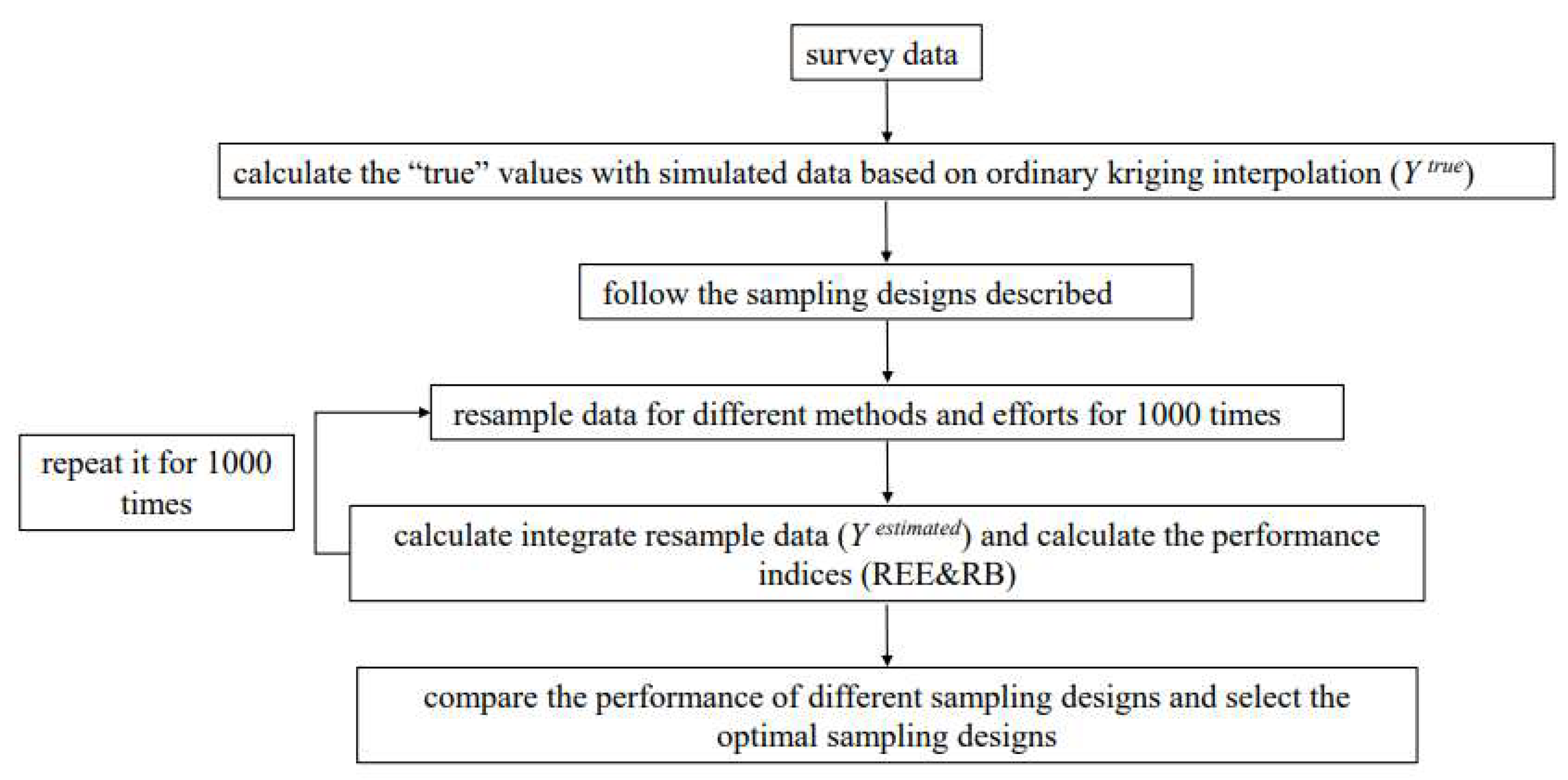
2.4. Simulation Procedure

The performances of different sampling designs in estimating the abundance indices of ichthyoplankton species were compared, and the consistency of the optimal sampling design in different years was evaluated. OKI was used to interpolate the relative abundance distribution of target ichthyoplankton species based on the original survey data, and the ‘true’ values (Y^true) of abundance indices were calculated based on the interpolated data. Different sampling methods were used to resample the interpolated data 1000 times at given sample sizes, and the estimated value of abundance indices of target species were calculated based on the resampled data. Relative estimation error (REE) and relative bias (RB) were used to compare the differences between the estimated values and ‘true’ values of abundance indices of target species for different sampling designs, and this process was repeated 1000 times. The optimal sampling designs were determined according to their performances in estimating abundance indices of ichthyoplankton species. The simulation process of this study is shown in the flowchart (Figure 3).

2.5. Measures for Evaluating Performance

Relative estimation error (REE) and relative bias (RB) were used to compare the performances of different sampling designs in estimating abundance indices of ichthyoplankton species in this simulation study. REE was used to evaluate the accuracy and precision of estimated abundance indices and was calculated as follows [52]:

$$\mathrm{REE}={\displaystyle \frac{\sqrt{{{\displaystyle \sum }}_{i=1}^R{\left(Y_i^{estimated}-Y^{true}\right)}^2/R}}{Y^{true}}}\times 100\%$$

(1)

RB was used for evaluating the accuracy of estimated abundance indices, and it can be calculated by the following formula [52,53]:

$$\mathrm{RB}={\displaystyle \frac{{{\displaystyle \sum }}_{i=1}^R{Y}_i^{estimated}/R-Y^{true}}{Y^{true}}}\times 100\%$$

(2)

where $Y^{true}$ is the ‘true’ value calculated based on the interpolated data, $Y_i^{estimated}$ is the estimated value calculated according to the ith resampled data, and R is the number of resampling times.

The optimal sampling designs were determined according to their general performances in estimating the abundance indices of all selected ichthyoplankton species at all levels of sample size. $T_{\overline{REE}}$ and $T_{\overline{\left|RB\right|}}$ is used to compared the performances of different sampling designs in estimating the abundance indices of multiple ichthyoplankton species in this study. $T_{\overline{REE}}$ is the sum of the average REE values of each single species under each sample size for all target species:

$$T_{\overline{REE}}={{\displaystyle \sum }}_{j=1}^J{{\displaystyle \sum }}_{k=1}^{K}MRE{E}_{jk}$$

(3)

where $MRE{E}_{jk}$ is the average REE values of the jth species at the kth level of sample size, J is the number of target species (J = 5), and K is the number of levels of sample size (K = 4).

$T_{\overline{\left|RB\right|}}$ is the sum of the average absolute value of RB (|RB|) at each sample size for all species, which is calculated as

$$T_{\overline{\left|RB\right|}}={\displaystyle \sum }_{j=1}^{J}Mean\left({{\displaystyle \sum }}_{k=1}^K{\displaystyle \frac{{{\displaystyle \sum }}_{i=1}^R\left|RB\right|}{R}}\right)$$

(4)

where J is the number of target species (J = 5), K is the number of levels of sample size (K = 4), and R is the number of resampling times at a given sample size.

3. Results

3.1. “True” Value of Spatiotemporal Distribution

Five species were chosen as the target species in the ichthyoplankton surveys in this study. These five fish species have similar spawning seasons, relatively high frequencies of occurrence, and different spatial distribution patterns over several years (

Table 2. The average abundances, standard deviations (SDs) and frequencies of occurrence of target ichthyoplankton species in the original surveys in different years.

Species	Scientific Name	Year	Average Abundance (ind./100 m3)	Standard Deviation (SD)	Frequency of Occurrence (%)
red tonguesole	Cynoglossus joyneri	2015	4.26	13.21	53.33
		2016	32.80	131.20	77.53
		2017	0.92	2.86	31.51
		2018	8.44	31.92	56.25
silver sillago	Sillago sihama	2015	5.15	28.17	48.89
		2016	10.39	37.78	77.53
		2017	10.12	46.67	50.69
		2018	1.36	5.20	37.50
Commerson’s anchovy	Stolephorus commersonni	2015	12.40	44.44	45.56
		2016	132.04	1014.07	59.55
		2017	5.72	23.85	36.99
		2018	83.90	437.97	54.17
dragonet	Callionymus·spp.	2015	9.31	27.06	27.78
		2016	3.14	11.92	25.84
		2017	9.75	33.26	30.14
		2018	10.70	51.72	31.25
Japanese anchovy	Engraulis japonicus	2015	12.31	78.46	25.56
		2016	7.26	36.64	49.44
		2017	8.58	29.12	64.38
		2018	14.21	62.02	43.75

).

The spatial distributions of five ichthyoplankton species’ abundances based on OKI in 2015 were shown to illustrate the spatial distribution of ‘true’ values of ichthyoplankton abundance in this study (Figure 4). The spatial distribution patterns of the different species differed significantly. In general, the silver sillago and Japanese anchovy were concentrated in the Haizhou Bay and its adjacent waters (Figure 4b,e), while Commerson’s anchovy was not only distributed in the Haizhou Bay but also had a higher abundance in the offshore waters of southern Jiangsu (Figure 4c); the high distribution area of the red tonguesole was concentrated in the northern waters of Jiangsu (Figure 4a), while the dragonet was concentrated in the north of the central and southern waters of the Yellow Sea (Figure 4d).

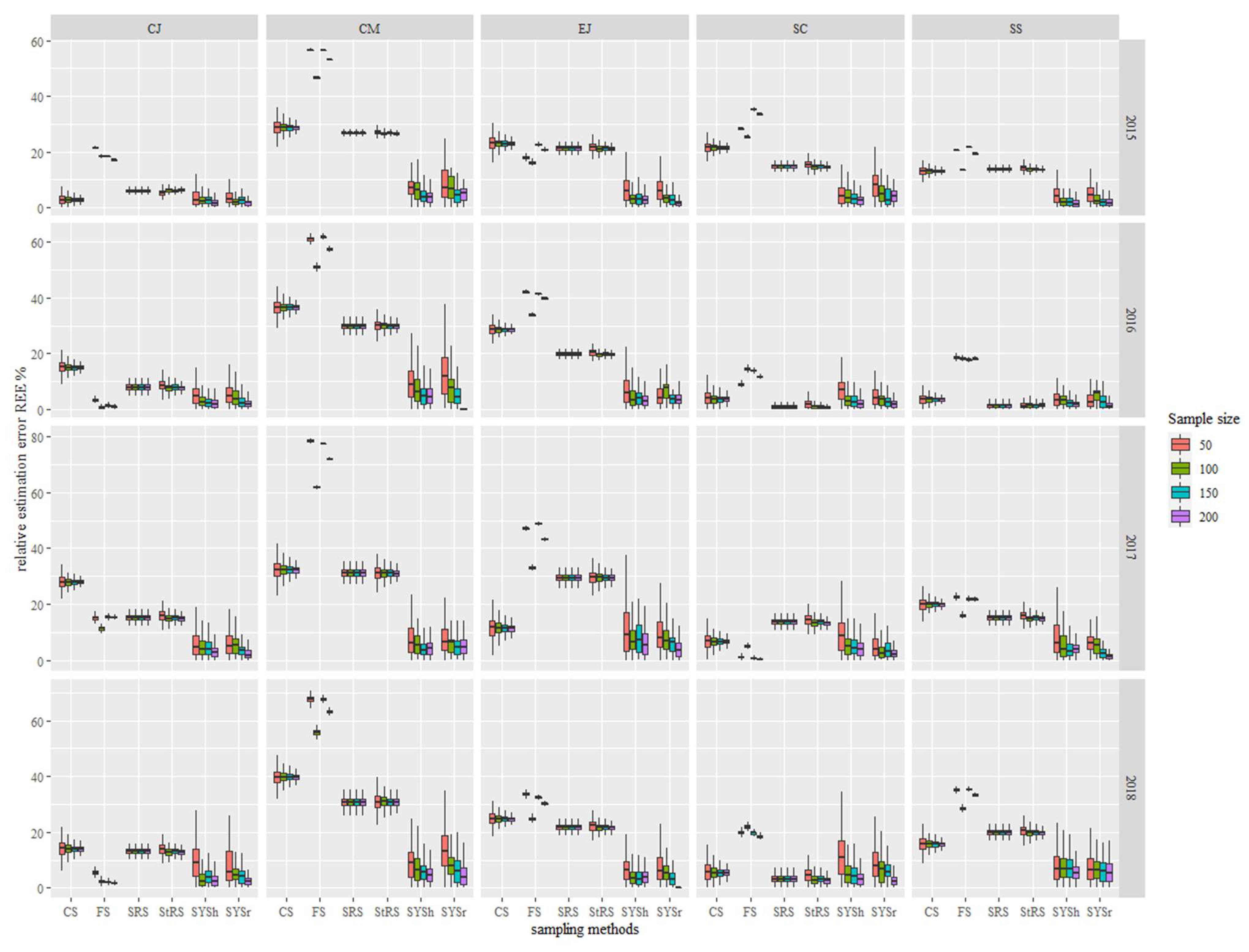
3.2. Comparison of REE

The REE values of abundance indices for target ichthyoplankton species in different sampling designs showed certain variations in different years (Figure 5). In general, except for fixed-station sampling methods, REE values in other sampling methods for target species were less than 30% at different sample sizes in different years. The REE values were relatively constant or showed decreasing trends with sample size.

The REE values in the different sampling designs varied for different species and in different years. For example, the REE values were relatively low and stable in CS in 2015 and relatively low in SYS in other years for red tonguesole (CJ) (Figure 5). For Commerson’s anchovy (SC), the REE values in SRS were low in 2016 and 2018, while the REE values in SYS were low in other years (Figure 5). For silver sillago (SS), the REE values of SRS in 2016 were at lower levels at small sample sizes, and SYS had better performances in other cases.

Compared with other sampling designs, the REE values of all target species in SYS were relatively low and showed slight annual variations (Figure 5). However, the REE ranges in SYS were relatively large at small sample sizes and low at large sample sizes. The performances of FS were unstable, and REE values were high for most of the target species over years and sensitive to sample size, except for a few cases like red tonguesole (CJ) in 2016 and Commerson’s anchovy (SC) in 2017. The REE values in FS did not show the decreasing tendency with sample size compared with those for other designs. SRS and StRS showed high stability, with the variability in REE values being small even at small sample sizes. However, the REE values in SRS and StRS were larger than those in SYS in most cases.

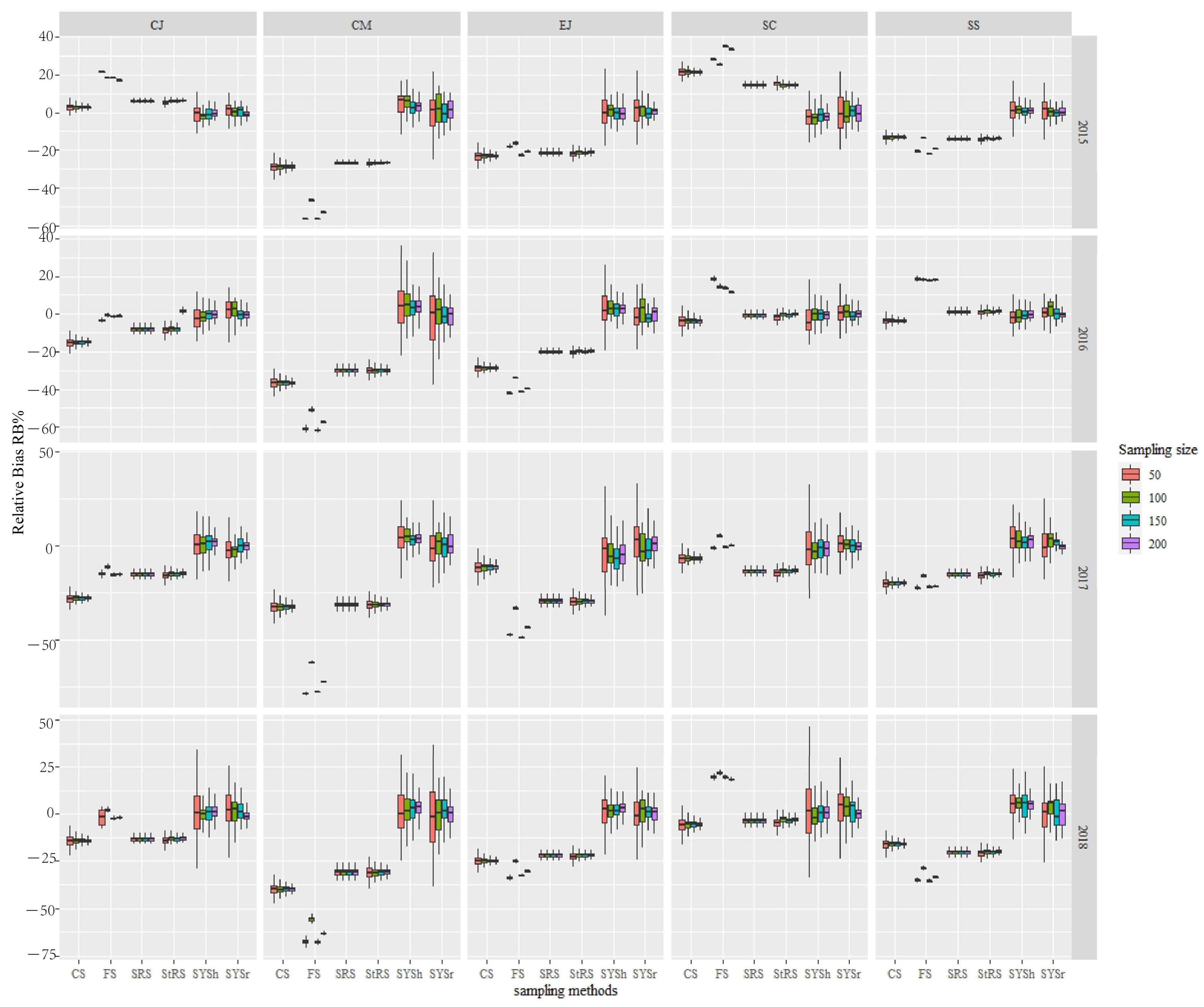
3.3. Comparison of RB

The RB values of estimated abundance indices of target ichthyoplankton species varied greatly in different sampling designs (Figure 6). The range of RB values generally decreased with sample size. The RB values of SYS fluctuated around zero, while the RB values in other sampling designs were either significantly higher or lower than zero in most cases.

The RB value of the estimation of the abundance indices of target ichthyoplankton species in FS differed greatly from zero in most cases, in which the abundance indices of target species were overestimated or underestimated, followed by cluster sampling design (CS), whose RB values deviated from zero. SRS and StRS had relatively small ranges of RB values, but the RB values in both designs deviated from zero. The RB values of SYS fluctuated around zero, without showing a consistently positive or negative trend with sample size. The fluctuation ranges of RB values in SYS were relatively large at relatively low sample sizes (Figure 6).

3.4. Comprehensive Comparison of Different Sampling Designs for Multiple Species

The $T_{\overline{REE}}$ values for the two systematic sampling designs were generally smaller than those in the other sampling designs in most years. As for the two systematic sampling designs, SYSh performed better in 2015 and in 2018 in terms of $T_{\overline{REE}}$, while SYSr was better than SYSh in terms of $T_{\overline{\left|RB\right|}}$ in 2017 and 2018. As for multiple species concerned, the performances of systematic sampling designs had relatively low interannual variations and high stability compared with those for single target species (

Table 3. The $T_{\overline{REE}}$ and $T_{\overline{\left|RB\right|}}$ of the estimated abundance indices of multiple ichthyoplankton species. FS, fixed-station sampling; SRS, simple random sampling; StRS, stratified random sampling; SYSh, hexagonal systematic sampling; SYSr, regular systematic sampling; CS, cluster sampling. $T_{\overline{REE}}$, the sum of the average REE values of each single species under each sample size for all target species; $T_{\overline{\left|RB\right|}}$, the sum of the average absolute value of RB (|RB|) at each sample size for all species.

Performance Index	Year	SRS	StRS	FS	CS	SYSh	SYSr
$T_{\overline{REE}}$	2015	82.90	82.89	140.83	89.38	18.64	21.31
	2016	60.99	60.48	129.17	87.61	21.98	21.88
	2017	106.78	105.97	170.81	111.45	28.63	26.92
	2018	106.63	105.85	163.12	110.09	30.58	31.29
$T_{\overline{\left|RB\right|}}$	2015	82.90	82.29	143.78	89.14	12.99	14.58
	2016	60.00	53.40	128.02	87.35	14.74	14.77
	2017	104.19	103.15	152.55	98.13	22.36	18.04
	2018	88.84	87.56	147.17	99.70	21.13	20.60

).

4. Discussion

This study showed that the two systematic sampling designs had better performances for estimating the abundance indices of multiple ichthyoplankton species compared with the other four sampling designs in terms of relative estimation error and relative bias in the ichthyoplankton survey. The results of the good performances of the systematic sampling designs were consistent with conclusions that were obtained in estuarine and benthic communities to estimate the population abundance index under different sampling designs [42,54]. Previous studies have suggested that SYS might underestimate the population density [8,54]. However, SYS showed unbiased estimates of abundance indices of ichthyoplankton species in this study. This may be due to the relatively high spatial coverage of sampling stations in SYS. In the case of ichthyoplankton, SYS can better cover the survey area, thus obtaining more data information. The performances in estimating abundance indices of ichthyoplankton species were similar for the two systematic sampling designs.

As for StRS and SRS, their performances in estimating abundance indices of ichthyoplankton species were relatively similar. In general, StRS performed better than SRS because it considered the low heterogeneity within strata and the high heterogeneity between strata. This study showed that StRS performed better than SRS in most cases, indicating that stratification was in line with the spatial distribution characteristics of target ichthyoplankton species in the study area to a certain extent, which was consistent with conclusions in previous studies [7,25,55,56].

Except for CJ, the abundance indices of other species in FS were seriously overestimated or underestimated in different years, while CS had a good sampling performance in some cases. CS is usually more applicable when the heterogeneity between transects is low and the heterogeneity within a transect is high [4,57]. Many studies have proposed developing adaptive sampling designs on the basis of CS to balance the sampling error of CS [4,58,59]. The REE and RB values in FS fluctuated within narrow ranges, which was due to random sampling out of the nine most adjacent stations in the space of fixed station points. However, the REE value in FS was the highest among all sampling designs, which may be due to the problem of station layout. If the spatial distribution of target ichthyoplankton species was relatively uniform, FS could reflect its interannual variation well [30,31]. However, fish species are often not uniformly distributed in the nature, so the sampling performance of FS usually shows great bias [7,28,29]. Currently, most studies on the ichthyoplankton were based on the data collected by the fixed-station sampling design [3,37,38]; however, this study showed that the fixed-station sampling design was likely to make the estimation of ichthyoplankton abundance less accurate. Therefore, it is necessary to evaluate the performances of current ichthyoplankton sampling program design and determine the optimal survey sampling design, so that higher-quality data can be obtained to conduct subsequent analysis.

In general, the estimated accuracy and precision of abundance indices of fish populations increase with sample size [25,59]. The REE values of estimates of abundance indices in SRS, StRS, and CS decreased slightly with sample size. However, REE values in SYS decreased largely and the fluctuation range became smaller with sample size in this study. The REE value of FS was smallest when the sample size was at 100 on most occasions, and it then increased even though the sample size increased to 150 sampling stations, which was not consistent with the general rule of sampling. The performances of SYS varied with species and years, and it had relatively high error in SYS for some sampling scenarios, which was consistent with previous studies [8,42]. As for SYS, SRS, or StRS, the REE values of abundance indices’ estimates of ichthyoplankton were small even at a small sample size, indicating that a relatively accurate estimate could be obtained even if the sample size was maintained at a low level for the ichthyoplankton survey. On the contrary, the REE values of abundance indices of target ichthyoplankton species in FS increased with sample size. Therefore, it is necessary to discuss the optimal sample size for different sampling designs specifically.

Larvae abundance is a relative index of spawning stock biomass, which can be used to monitor the population dynamics of fish species, and can provide basic information for the designation of protected areas and fisheries management [60]. When faced with multiple survey objectives, the optimal sampling designs are often different for different sampling objectives [7,25,61]. For the long-term fishery-independent survey, especially for ichthyoplankton, which is passively transported [62], the performance of survey design needs to be continuously evaluated and re-examined to ensure the accuracy of the survey data due to the possible changes in spatial distribution caused by environmental change and changes in the adaptability of the fish themselves [63].

The defined strata in StRS referred to the spatial structure of the ichthyoplankton community in the coastal waters of the central and southern Yellow Sea in this study [38]. However, the spatial distribution of species abundance might be different from the spatial pattern at community level. This may explain why StRS did not perform better than SRS in estimating abundance indices of target fish populations on some occasions. Many studies indicated that it was necessary to adjust the strata to obtain the optimal stratification design when aiming at different sampling objectives [7,25,64]. The effect of stratification scheme on the estimation of abundance indices of target ichthyoplankton species should be furtherly examined in future studies.

In this study, the abundance indices of ichthyoplankton species were used as the sampling objective to evaluate the performances of different sampling designs. SYS is the most suitable sampling method for the ichthyoplankton survey program. This study provided a framework to determine a reasonable sampling design for estimating the abundance indices of target ichthyoplankton species in the ichthyoplankton survey.

5. Conclusions

This study explored the effects of different sampling designs on the population abundance estimation of ichthyoplankton in the coastal waters. The two systematic sampling designs were better than the other four traditional sampling designs in estimating the abundance of different ichthyoplankton species. This suggests that the sampling design that evenly covers the entire sea area, including both the high- and low-value areas of the species distribution, is optimal when estimating ichthyoplankton species abundance in an ichthyoplankton sampling program. The findings can be used to propose a method with higher precision and accuracy for ichthyoplankton surveys and to reduce the survey cost in case of being able to obtain accurate data, as well as to provide a sampling program reference for further ichthyoplankton surveys.

References

1. Cochran, W.G. Sampling Techniques, 3rd ed.; John Wiley & Sons: New York, NY, USA, 1977; pp. 18–322. [Google Scholar]
2. Rago, P.J. Fishery independent sampling: Survey techniques and data analyses. FAO Fish. Technical. 2005, 474, 201–215. [Google Scholar]
3. Bazigos, G.; Kavadas, S. Optimal sampling designs for large-scale fishery sample surveys in Greece. Mediterr. Mar. Sci. 2007, 8, 65–84. [Google Scholar] [CrossRef]
4. King, S.E.; Powell, E.N. Influence of adaptive stations in a transect-based sampling design for a multispecies fish survey. Fish. Res. 2007, 86, 241–261. [Google Scholar] [CrossRef]
5. Yu, H.; Jiao, Y.; Su, Z.; Reid, K. Performance comparison of traditional sampling designs and adaptive sampling designs for fishery-independent surveys: A simulation study. Fish. Res. 2012, 113, 173–181. [Google Scholar] [CrossRef]
6. Xu, B.; Ren, Y.; Chen, Y.; Xue, Y.; Zhang, C.; Wan, R. Optimization of stratification scheme for a fishery-independent survey with multiple objectives. Acta Oceanol. Sin. 2015, 34, 154–169. [Google Scholar] [CrossRef]
7. Wang, J.; Xu, B.; Zhang, C.; Xue, Y.; Chen, Y.; Ren, Y. Evaluation of alternative stratifications for a stratified random fishery-independent survey. Fish. Res. 2018, 207, 150–159. [Google Scholar] [CrossRef]
8. Ma, J.; Tian, S.; Gao, C.; Richard, K.; Zhao, J. Evaluation of sampling designs for different fishery groups in the Yangtze River estuary, China. Reg. Stud. Mar. Sci. 2020, 38, 10373. [Google Scholar] [CrossRef]
9. Garcia, A.M.; Vieira, J.P.; Winemiller, K.O. Effects of 1997–1998 El Niño on the dynamics of the shallow-water fish assemblage of the Patos Lagoon Estuary (Brazil). Estuar. Coast. Shelf Sci. 2003, 57, 489–500. [Google Scholar] [CrossRef]
10. Rabbaniha, M.; Molinero, J.C.; Lopez-Lopez, L.; Javidpour, J.; Primo, A.L.; Owfi, F.; Sommer, U. Habitat association of larval fish assemblages in the northern Persian Gulf. Mar. Pollut. 2015, 97, 105–110. [Google Scholar] [CrossRef] [PubMed]
11. Marina, B.; Svetlana, K.; Francesco, F. The long-term ichthyoplankton abundance summer trends in the coastal waters of the Black Sea under conditions of hydrometeorological changes. Estuar. Coast. Shelf Sci. 2021, 258, 107450. [Google Scholar] [CrossRef]
12. Smith, P.E.; Richardson, S.L. Standard Techniques for Pelagic Fish Egg and Larval Surveys. FAO Fish. Tech. Pap. 1997, 175, 6–113. [Google Scholar]
13. Stratoudakis, Y.; Bernal, M.; Ganias, K.; Uriarte, A. The daily egg production method: Recent advances, current applications and future challenges. Fish Fish. 2006, 7, 35–57. [Google Scholar] [CrossRef]
14. Guerchon, J.; Morov, A.R.; Tagar, A.; Rubin-Blum, M.; Tikochinski, Y.; Berenshtein, I.; Rilov, G.; Stern, N. Marine top secrets: Ichthyoplankton in surface water uncover hidden knowledge on fish diversity and distribution. Estuar. Coast. Shelf Sci. 2023, 282, 108226. [Google Scholar] [CrossRef]
15. Heath, M.R. Field Investigations of the Early Life Stages of Marine Fish. In Advances in Marine Biology; Academic Press: Salt Lake City, UT, USA, 1992; pp. 10–169. [Google Scholar]
16. Edwards, M.; Beaugrand, G.; Hays, G.C.; Koslow, J.A.; Richardson, A.J. Multi-decadal oceanic ecological datasets and their application in marine policy and management. Trends Ecol. Evol. 2010, 25, 602–610. [Google Scholar] [CrossRef] [PubMed]
17. Zhan, B. Fishery Stock Assessment; China Agriculture Press: Beijing, China, 1995; pp. 261–262. [Google Scholar]
18. Zhang, C.I.; Lee, J.B. Stock assessment and management implications of horse mackerel (Trachurus japonicus) in Korean waters, based on the relationships between recruitment and the ocean environment. Prog. Oceanogr. 2001, 49, 513–537. [Google Scholar] [CrossRef]
19. Sassa, C.; Konishi, Y.; Mori, K.E.N. Distribution of jack mackerel (Trachurus japonicus) larvae and juveniles in the East China Sea, with special reference to the larval transport by the Kuroshio Current. Fish. Oceanogr. 2006, 15, 508–518. [Google Scholar] [CrossRef]
20. Pepin, P.; Helbig, J.A. Sampling variability of ichthyoplankton surveys—Exploring the roles of scale and resolution on uncertainty. Fish. Res. 2012, 117–118, 137–145. [Google Scholar] [CrossRef]
21. Arbia, G.; Lafratta, G. Anisotropic spatial sampling designs for urban pollution. J. R. Stat. Soc. 2002, 51, 223–234. [Google Scholar] [CrossRef]
22. Li, M.; Zhang, C.; Xu, B.; Xue, Y.; Ren, Y. Evaluating the approaches of habitat suitability modelling for whitespotted conger (Conger myriaster). Fish. Res. 2017, 195, 230–237. [Google Scholar] [CrossRef]
23. Cadima, E.; Caramelo, A.; Afonso-Dias, M.; Tandstad, M.; Leiva-Moreno, J. Sampling methods applied to fisheries science: A manual. In FAO Fisheries Technical Paper; Food & Agriculture Organization: Rome, Italy, 2005; Volume 434, Available online: https://agris.fao.org/search/en/records/65dde2400f3e94b9e5c6baf8 (accessed on 17 April 2021).
24. Smith, S.J.; Tremblay, M.J. Fishery-independent trap surveys of lobsters (Homarus americanus): Design considerations. Fish. Res. 2003, 62, 65–75. [Google Scholar] [CrossRef]
25. Xu, B.; Zhang, C.; Xue, Y.; Ren, Y.; Chen, Y. Optimization of sampling effort for a fishery-independent survey with multiple goals. Environ. Monit. Assess. 2015, 187, 252. [Google Scholar] [CrossRef] [PubMed]
26. Zhao, J.; Cao, J.; Tian, S.; Chen, Y.; Zhang, S. Evaluating sampling designs for demersal fish communities. Sustainability 2018, 10, 2585. [Google Scholar] [CrossRef]
27. Zhao, J.; Zhang, S.; Lin, J.; Zhou, X. A comparative study of different sampling designs in fish community estimation. Chin. J. Appl. Ecol. 2014, 25, 1181–1187. [Google Scholar]
28. Sun, C.; Wang, Y. Impacts of sampling design on the abundance estimation of Portunus trituberculatus using crab pots. J. Oceanol. Limnol. 2020, 39, 770–783. [Google Scholar] [CrossRef]
29. Sun, C.; Wang, Y. Impacts of the sampling design on the abundance index estimation of Portunus trituberculatus using bottom trawl. Acta Oceanol. Sin. 2020, 39, 48–57. [Google Scholar] [CrossRef]
30. Flint, R.W.; Holland, J.S. Benthic infaunal variability on a transect in the Gulf of Mexico. Estuar. Coast. Mar. Sci. 1980, 10, 1–14. [Google Scholar] [CrossRef]
31. Hawthorne, S.D.; Dauer, D.M. Macrobenthic communities of the lower Chesapeake Bay. IV. Bay-wide transects and the inner continental shelf. Benthic Stud. Low. Chesap. Bay 1984, 68, 193–205. [Google Scholar] [CrossRef]
32. Fuller, W.A. Environmental surveys over time. J. Agric. Biol. Environ. Stat. 1999, 4, 331–345. [Google Scholar] [CrossRef]
33. McCormick, J.L.; Quist, M.C.; Schill, D.J. Creel survey sampling designs for estimating effort in short-duration chinook salmon fisheries. N. Am. J. Fish. Manag. 2013, 33, 977–993. [Google Scholar] [CrossRef]
34. Cheng, Z.; Gao, L.; Yu, L.; Duan, X.; Zhu, F.; Tian, H.; Chen, D.; Liu, M. Catch Efficiency of Multi-Mesh Trammel Nets for Sampling Freshwater Fishes. Fishes 2023, 8, 464. [Google Scholar] [CrossRef]
35. Hernandez, F.J.; Carassou, L.; Muffelman, S.; Powers, S.P.; Graham, W.M. Comparison of two plankton net mesh sizes for ichthyoplankton collection in the northern Gulf of Mexico. Fish. Res. 2011, 108, 327–335. [Google Scholar] [CrossRef]
36. Koslow, J.A.; Wright, M. Ichthyoplankton sampling design to monitor marine fish populations and communities. Mar. Policy 2016, 68, 55–64. [Google Scholar] [CrossRef]
37. Wei, Y.; Wang, X.; Zhang, H.; Liu, L.; Cai, Y. Ichthyoplankton species composition and distribution in Hangzhou Bay in summer during 2004~2010. J. Oceanogr. Taiwan Strait 2012, 31, 501–508. [Google Scholar] [CrossRef]
38. Xiao, H.; Zhang, C.; Xue, Y.; Xu, B.; Yu, H.; Ren, Y. Community structure of ichthyoplankton from typical transects in Haizhou Bay and its adjacent waters during spring and summer. J. Fish. Sci. China 2017, 24, 1079–1090. [Google Scholar] [CrossRef]
39. Kuriyama, P.T.; Sugihara, G.; Thompson, A.R.; Semmens, B.X. Identification of shared spatial dynamics in temperature, salinity, and ichthyoplankton community diversity in the California Current System with empirical dynamic modeling. Front. Mar. Sci. 2020, 7, 1–17. [Google Scholar] [CrossRef]
40. Long, X.; Wan, R.; Li, Z.; Wang, D.; Song, P.; Zhang, F. Sampling designs for monitoring ichthyoplankton in the estuary area: A case study on Coilia mystus in the Yangtze Estuary. Front. Mar. Sci. 2022, 8, 767273. [Google Scholar] [CrossRef]
41. Dorner, B.; Holt, K.R.; Peterman, R.M.; Jordan, C.; Larsen, D.P.; Olsen, A.R.; Abdul-Aziz, O.I. Evaluating alternative methods for monitoring and estimating responses of salmon productivity in the North Pacific to future climatic change and other processes: A simulation study. Fish. Res. 2013, 147, 10–23. [Google Scholar] [CrossRef]
42. Cao, J.; Chen, Y.; Chang, J.H.; Chen, X. An evaluation of an inshore bottom trawl survey design for American lobster (Homarus americanus) using computer simulations. J. N. Atl. Fish. Sci. 2014, 46, 27–39. [Google Scholar] [CrossRef]
43. Wan, R.; Jiang, Y. Studies on the ecology of eggs and larval of Osteichithyes in the Yellow Sea. Mar. Fish. Res. 1998, 19, 60–73. [Google Scholar]
44. Chen, J.; Xu, Z.; Chen, X. Zooplankton in the coast waters of southern Yellow Sea during winter and spring. Mar. Fish. 2008, 30, 327–332. [Google Scholar] [CrossRef]
45. Tang, Q. Regional Oceanography in China: Fishery Oceanography; Ocean Press: Beijing, China, 2012; pp. 16–17. [Google Scholar]
46. General Administration of Quality Supervision, Inspection and Quarantine of the People’s Republic of China. Specifications for Oceanographic Survey-Part 6: Marine Biological Survey GB/T 12763. 6-2007; China Standard Press: Beijing, China, 2007. [Google Scholar]
47. Zhao, C.; Zhang, R.; Lu, S. Fish Eggs and Larvae in China Seas, 2nd ed.; Shanghai Scientific and Technical Publishers: Shanghai, China, 1985; pp. 18–188. [Google Scholar]
48. Wan, R.; Zhang, R. Eggs and Larvae of Fish in the Coastal and Adjacent Waters of China; Shanghai Scientific and Technical Publishers: Shanghai, China, 2017; pp. 45–435. [Google Scholar]
49. Schabenberger, O.; Gotway, C. Statistical Methods for Spatial Data Analysis; Chapman and Hall: London, UK, 2005; pp. 23–100. [Google Scholar]
50. Oliver, M.A.; Webster, R. Kriging: A method of interpolation for geographical information systems. Int. J. Geogr. Inf. Syst. 1990, 4, 313–332. [Google Scholar] [CrossRef]
51. Pokhrel, R.M.; Kuwano, J.; Tachibana, S. A kriging method of interpolation used to map liquefaction potential over alluvial ground. Eng. Geol. 2013, 152, 26–37. [Google Scholar] [CrossRef]
52. Chen, Y. A Monte Carlo study on impacts of the size of subsample catch on estimation of fish stock parameters. Fish. Res. 1996, 26, 207–223. [Google Scholar] [CrossRef]
53. Jiao, Y.; Chen, Y.; Schneider, D.; Wroblewski, J. A simulation study of impacts of error structure on modeling stock–recruitment data using generalized linear models. Can. Fish. Aquat. Sci. 2004, 61, 122–133. [Google Scholar] [CrossRef]
54. Hyun, S.-Y.; Seo, Y.I.L. The systematic sampling for inferring the survey indices of Korean groundfish stocks. Fish. Aquat. Sci. 2018, 21, 24. [Google Scholar] [CrossRef]
55. Chen, Y.; Sherman, S.; Wilson, C.; Sowles, J. A comparison of two fishery-independent survey programs used to define the population structure of American lobster (Homarus americanus) in the Gulf of Maine. Fish. Bull. 2006, 104, 247–255. [Google Scholar]
56. Miller, T.J.; Skalski, J.R.; Ianelli, J.N. Optimizing a stratified sampling design when faced with multiple objectives. Ices J. Mar. Sci. 2007, 64, 97–110. [Google Scholar] [CrossRef]
57. Li, B.; Cao, J.; Chang, J.-H.; Wilson, C.; Chen, Y. Evaluation of effectiveness of fixed-station sampling for monitoring American lobster settlement. N. Am. J. Fish. Manag. 2015, 35, 942–957. [Google Scholar] [CrossRef]
58. Pollard, J.H.; Palka, D.; Buckland, S.T. Adaptive line transect sampling. Biometrics 2002, 58, 862–870. [Google Scholar] [CrossRef]
59. Moradi, M. Using adaptive line-transect sampling in airborne geophysics studies. Commun. Stat.-Simul. Comput. 2019, 48, 675–683. [Google Scholar] [CrossRef]
60. Smith, S.; Lundy, M. Improving the precision of design-based scallop drag surveys using adaptive allocation methods. Can. J. Fish. Aquat. Sci. 2006, 63, 1639–1646. [Google Scholar] [CrossRef]
61. Zhang, G.; Wang, J.; Xue, Y.; Zhang, C.; Xu, B.; Cheng, Y.; Ren, Y. Comparison of sampling effort allocation strategies in a stratified random survey with multiple objectives. Aquac. Fish. 2020, 5, 113–121. [Google Scholar] [CrossRef]
62. Xing, Q.; Yu, H.; Yu, H.; Sun, P.; Liu, Y.; Ye, Z.; Li, J.; Tian, Y. A comprehensive model-based index for identification of larval retention areas: A case study for Japanese anchovy Engraulis japonicus in the Yellow Sea. Ecol. Indic. 2020, 116, 106479. [Google Scholar] [CrossRef]
63. Davidson, E.R.; Hussey, N.E. Movements of a potential fishery resource, porcupine crab (Neolithodes grimaldii) in Northern Davis Strait, Eastern Canadian Arctic. Deep-Sea Res. Pt. I 2019, 154, 103143. [Google Scholar] [CrossRef]
64. Singh, T.; Kumar, R. Allocation of Sample in Stratified Sampling using Circular Systematic Sampling. J. Indian Soc. Agric. Stat. 2017, 71, 61–65. [Google Scholar]
Figure 1. The sampling stations of the ichthyoplankton survey in the coastal waters of the central and southern Yellow Sea from 2015 to 2018.
Fishes 10 00039 g001
Figure 2. The example maps of different sampling designs under 50 sampling stations. (a) stratified random sampling (StRS) design; Zone A, Haizhou Bay and its adjacent waters (34.5°~35.75° N, 119.3°~121° E); zone B, the coastal waters of northern Jiangsu Province (33.00°~34.50° N, 121°~122° E); zone C, the coastal waters of southern Jiangsu Province (32.00°~33.00° N, 122°~123° E); (b) fixed-station sampling design (FS); (c) cluster sampling (CS) design; (d) regular systematic sampling (SYSr) design; (e) hexagonal systematic sampling (SYSh) design.
Fishes 10 00039 g002
Figure 3. The flowchart of the simulation study on evaluating different sampling designs in estimating the abundances of multiple target species in the ichthyoplankton survey.
Fishes 10 00039 g003
Figure 4. The spatial distribution of the abundance data (ind./100 m3) of target ichthyoplankton species based on ordinary kriging interpolation in 2015 in the coastal waters of the central and southern Yellow Sea: (a) CJ, red tonguesole; (b) SS, silver sillago; (c) SC, Commerson’s anchovy; (d) CM, Dragonet·spp; (e) EJ, Japanese anchovy.
Fishes 10 00039 g004
Figure 5. The relative estimation error (REE) for different target species with different sampling designs in different years. FS, fixed-station sampling; SRS, simple random sampling; StRS, stratified random sampling; SYSh, hexagonal systematic sampling; SYSr, regular systematic sampling; CS, cluster sampling. CJ, red tonguesole; CM, dragonet; EJ, Japanese anchovy; SS, silver sillago; SC, Commerson’s anchovy.
Fishes 10 00039 g005
Figure 6. The relative bias (RB) for different species with different sampling designs in different years. FS, fixed-station sampling; SRS, simple random sampling; StRS, stratified random sampling; SYSh, hexagonal systematic sampling; SYSr, regular systematic sampling; CS, cluster sampling. CJ, red tonguesole; CM, dragonet; EJ, Japanese anchovy; SS, silver sillago; SC, Commerson’s anchovy.
Fishes 10 00039 g006