Research on Improved Near-Infrared Fish Density Classification Method Based on ResNet18

Abstract

Addressing the technological requirement for real-time monitoring of fish density in dim aquaculture environments, this study proposes a near-infrared (NIR) image classification method using a modified ResNet18 architecture. Initially, an NIR-Fish dataset comprising 736 high-quality annotated images (256 × 256 resolution) spanning three density scenarios (low, medium, and high density) was constructed. Contrast-Limited Adaptive Histogram Equalization (CLAHE) preprocessing was implemented with an 8 × 8 tiling strategy and clip limit = 4.0, significantly enhancing the discernibility of faint boundary features. A dual-channel attention module (DCAM) was embedded into the ResNet18 backbone, featuring a parallel architecture integrating Global Average Pooling (GAP) and Global Max Pooling (GMP). This design synergistically optimized local salient feature enhancement and global statistical feature fusion through parameter-shared fully connected layers (reduction ratio of 16:1). The experiments show that the classification accuracy of the proposed method on the independent test set is 80.57%, which is 4.34 percentage points higher than that of the original ResNet18. F1 scores for the three density levels were 0.8308 (low), 0.7674 (medium), and 0.8294 (high), respectively. Ablation studies confirmed the dual-channel design’s significant performance contribution, while the parameter-sharing mechanism effectively mitigated overfitting risks. By leveraging feature complementarity and lightweight design, this work overcomes the classification bottleneck for NIR images under low signal-to-noise conditions, providing a highly robust technical solution for intelligent aquaculture management.

1. Introduction

The continuous growth of the global population and rising living standards have significantly increased the demand for aquatic products, thereby driving the rapid development of aquaculture. According to statistics from the International Fisheries Organization, the global total production of fisheries and aquaculture reached 214 million tons in 2020, of which aquatic animal production accounted for 178 million tons. It is projected that by 2030, the total production of aquatic animals will further increase to 202 million tons [1]. As fish constitute nearly seventy percent of aquatic animals, enhancing fish farming management efficiency and yield has become a key challenge. Traditional manual farming methods suffer from inefficiency and high costs [2], making them unsuitable for modern large-scale aquaculture. These limitations have propelled the transition towards unmanned and automated fish farming. In particular, with the rapid advancement of computer and information technologies, intelligent farming has become a trending research hotspot, with its core lying in the precise assessment of fish feeding intensity. Most existing research on intelligent fish farming technologies has been conducted under well-lit conditions [3]. However, not all aquaculture environments possess sufficient lighting, and certain fish species are unsuitable for growth in brightly lit conditions. Research on analyzing fish feeding intensity using near-infrared vision technology under low-light conditions is relatively scarce, and the accuracy and robustness of existing studies are suboptimal. Therefore, designing specific algorithms for fish feeding intensity assessment that account for the imaging characteristics of NIR technology is crucial to improve evaluation accuracy.

Near-infrared vision technology has shown significant advantages in solving dark or nighttime fish observation. Related studies show that an 850 nm near-infrared light source has no significant effect on fish behavior, which provides a theoretical basis for the monitoring of dark light environments [4], and its cross-domain application has verified the universality of the technology. For example, 730 nm single-wavelength imaging in agriculture can identify cherry fruit fly oviposition damage [5]. The 850 nm band is used in animal husbandry to detect organic acids in silage [6]. The subcutaneous vascular network is extracted by the matched filter enhancement technique in the medical field [7]. However, aquatic NIR imaging faces unique challenges: First, low contrast results in blurred fish contours [8]. Secondly, random electrical noise interferes with feature extraction [9]. Finally, NIR imaging also has dynamic disturbances, such as the clumping of bait. Addressing the aforementioned challenges, we present a systematic framework wherein image enhancement techniques are utilized to refine raw data quality (Section 2.1), followed by a dual-channel attention mechanism engineered to optimize feature representation (Section 2.2).

For the technical aspects of visible light computer vision, Saminiano et al. set two predefined labels: feeding and not feeding. The convolutional neural network algorithm is used to classify the feeding status of fish individual images, and its accuracy can reach 96.4% [10]. In order to further refine the intensity of fish feeding activity, Ubina et al. further refined the labels and realized the identification of four different levels of feeding intensity: none, weak, moderate, and strong. The optical flow neural network is used to generate optical flow frames instead of fish images as the input images of the feeding behavior recognition network, and the final accuracy can reach 95% [11]. Tang et al. used the optical flow method for feature extraction to achieve three classifications of underwater fish feeding status and two classifications of aquatic fish feeding status [12]. Xu et al.improved the deep learning model LRCN by integrating the SE (squeeze-and-excitation network) attention module into LRCN, improving the feature picking ability of the model for the classification of fish feeding behavior and realizing the three classification of the water feeding status [13]. Based on the lightweight neural network MobileViT, Xu et al. combined the CBAM attention module with the MV2 module to design the CBAM-MV2 module, which improved the prediction ability, robustness, and generalization performance of the model, and the accuracy can reach 98.61% [14].

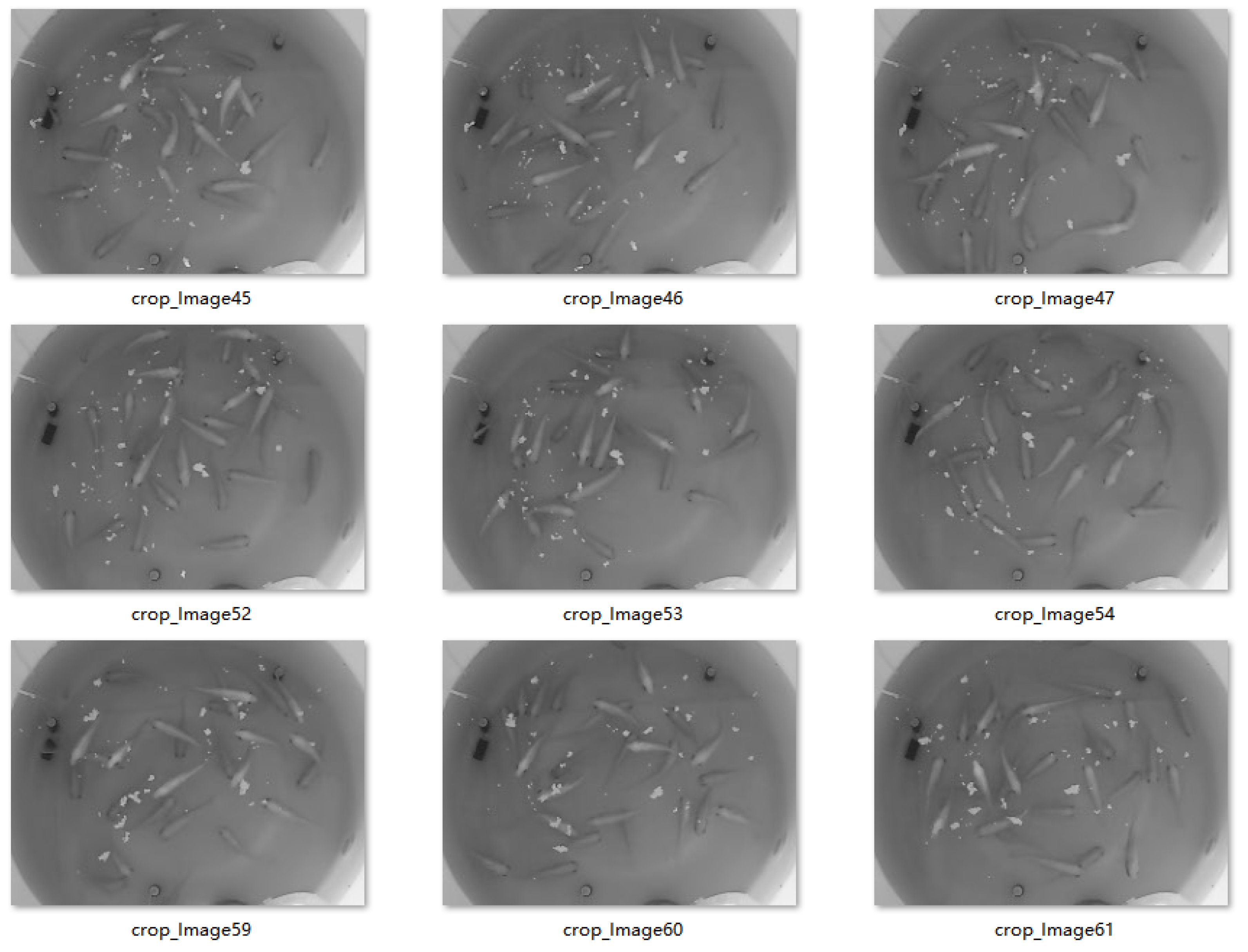
For infrared vision, Zhou et al. [15] analyzed the feeding behavior of the fish school based on the obtained near-infrared image and divided the image into background and fish school. Firstly, the order moment is used to calculate the centroid of the fish school, which is used as the vertex for triangulation, and then, the fish density index is calculated as the quantitative index of feeding behavior. Since the texture features of the water surface can reflect the spatial information of fish, such as the direction of movement and the range of change, the texture features of the image can also be extracted by the gray level co-occurrence matrix to characterize the feeding intensity of fish. Finally, the feeding intensity of fish is quantified by combining the degree of fish density with the texture features of the water surface.The near-infrared fish feeding image is shown in Figure 1. Zheng et al. [16], on the other hand, proposed a method for fish feeding intensity assessment based on near-infrared depth maps, which mainly collect depth information of fish schools through depth cameras. Then, according to the depth map obtained, the fish foreground object can be extracted, and the background image can be eliminated with the minimum amount of calculation so as to obtain a clear fish feeding image. This method estimates the number of preying fish by the total number of target pixels in the depth map and combines the change rate of target pixels to reflect the feeding activity of fish in real time.

In the research of fish feeding behavior recognition, the attention mechanism, as a key technology for improving the feature selection ability of the model, has shown significant advantages in various visual tasks in recent years. For example, the multi-level cross-attention feature proposed by Hosam et al. realizes cross-scale feature interaction through a two-branch transformer [17] and achieves 99.91% recognition accuracy in the PlantVillage dataset, which is especially suitable for the feature separation problem between fish and complex water bodies in infrared images. Dynamic Threshold Convolution and Multi-Path Dynamic Attention developed by Yang et al. achieve 99.50% accuracy on the Tiny-ImageNet dataset by filtering water interference features through key token selection strategies [18]. He et al. designed Autocorrelation Attention and Cross-Spatial Correlation Attention for small sample scenes, which improved the classification accuracy by 2.41% in small sample datasets, and they provided a solution for aquaculture scenes with scarce annotations [19]. The Spatial Location Channel Attention Module (SLCAM) designed by Xu et al. uses a four-branch architecture to simultaneously extract horizontal and vertical spatial features, and its bidirectional pooling strategy improves the Top-1 accuracy of ResNet50 by 2.52% on ImageNet-1K [20]. This feature can enhance the contour localization ability of the model for near-infrared image data. Fu et al. combined channel–spatial attention and CNN–transformer architecture in hyperspectral classification, and they achieved 92.84% mAP in the Honghu dataset, which effectively solved the problem of background interference in cross-modal feature fusion [21]. The residual group Multi-Scale Enhanced Attention Network of Wang et al. combines coordinate attention and improved tensor synthetic attention to achieve 96.88% accuracy on the CIFAR-10 dataset, and the inference speed is increased by 1.8 times, which results in subsequent lightweight subsequent models [22]. Loosen Attention designed by Wang et al. for aurora images improves the classification accuracy by 15.9% under 4k sample training through the fusion of localized channel attention and coarse-grained spatial attention. This dynamic feature adaptation mechanism is particularly suitable for water body fluctuation scenes [23]. Wang et al.’s Multi-Scale Frequency Attention Fusion network combined with Spatial Frequency Attention module achieves 7.25 EN value on the MSRS dataset, which significantly enhances the model’s ability to retain texture features of images [24].

Studies have shown that fish feeding intensity is highly correlated with the density of fish. When fish are feeding, they will gather in shallow water [25]. However, when the fish in the breeding pond are not feeding, they will potentially roam underwater. An accurate classification of the density degree of shallow fish schools will help assess fish feeding intensities. In this study, based on the image classification model of deep learning, the fully supervised learning strategy is used to accurately classify the fish density degree. By constructing high-quality labeled datasets, the model still shows excellent robustness and generalization ability under limited labeled samples. This method can provide objective and consistent classification results, accurately meet the needs of fish density monitoring, and is of great significance for promoting the intelligent management of aquaculture.

2. Materials and Methods

2.1. Dataset Construction

The NIR-Fish dataset constructed in this study is derived from a simulated farming system in a laboratory environment, and the experimental device includes a circular farming barrel with a diameter of 1.2 m, an oxygen booster, a water changer, and a camera with near-infrared vision shooting function. The experimental subjects were groups of grass goldfish with a body length of 10–15 cm. Before data collection, a 72 h feeding cessation treatment was implemented to ensure that feeding behavior was accurately triggered by experimental feeding. The camera was set up 0.8 m above the breeding bucket, and dynamic changes in the fish from a static state to density feeding during the feeding process were recorded at a frame rate of 30 fps. The total duration of the video covered the critical response period of 0–600 s after feeding. The original data is constructed by the sequential frame extraction strategy, and key frames of the video are extracted at an interval of 5 s. After the dithering process, 736 valid images are obtained. 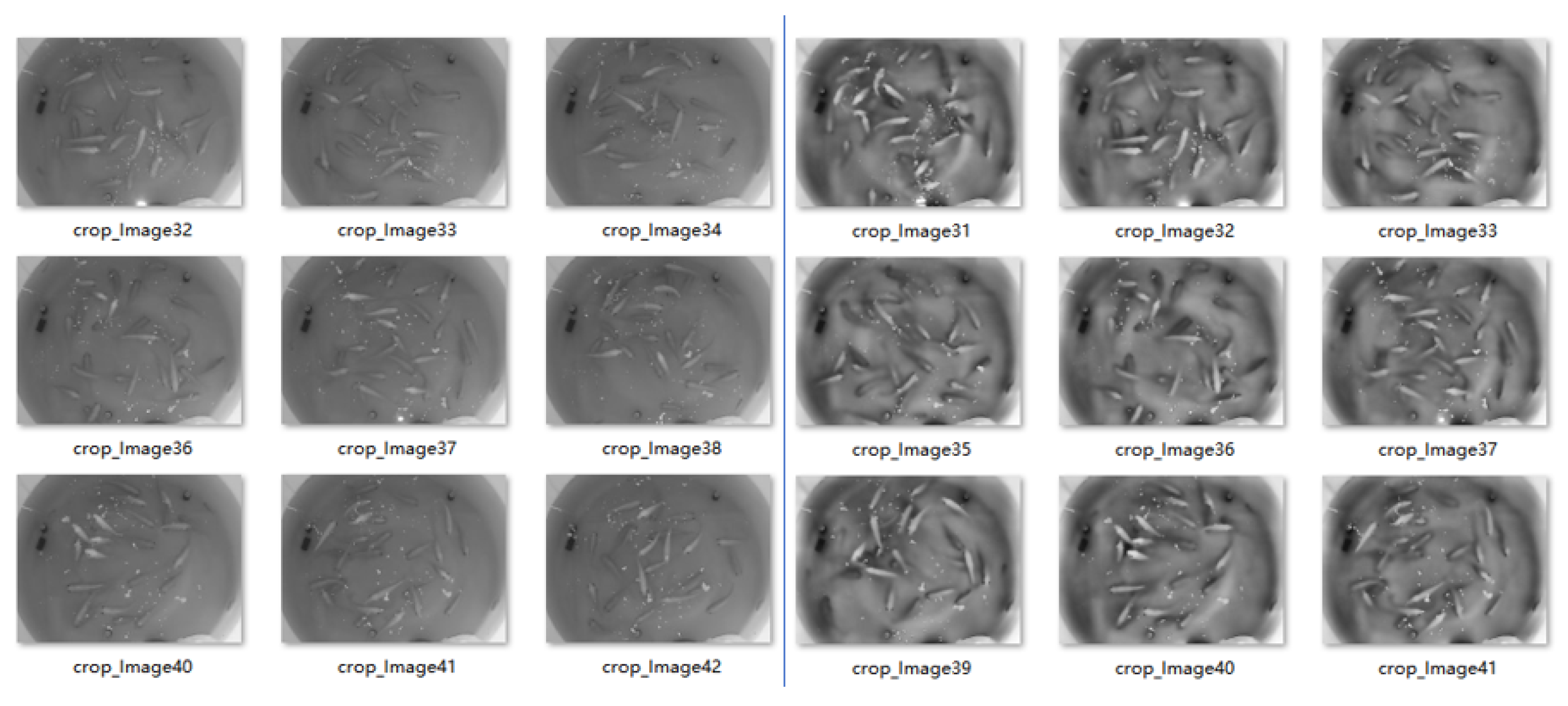An example of the collected dataset is shown in Figure 1. It can be seen from the collected image data that the contrast in a single image is low, and the discrimination of fish density degree between different images is not obvious. It is necessary to enhance the characteristics of fish density degree in the image by preprocessing.

In this study, the Contrast-Limited Adaptive Histogram Equalization (CLAHE) method is used for image enhancement. The CLAHE algorithm works by cutting the whole image into many small squares to adjust the contrast inside each cube individually [26]. This local adaptive strategy has been proven to be effective in preserving key detail features in medical image enhancement [27]. It is worth noting that the choice of the tile’s size is a trade-off: If the cubes are too large, the adjustment will not be fine enough. If the small square is too small, it will produce obvious square traces again. For example, in the study of strawberry phenotype classification, Yang et al.found that the block size of CLAHE had a significant impact on the accuracy of organ recognition. When 4 × 4 small blocks were used, the junction of the strawberry fruit and calyx easily produced splitting artifacts, which led to the distortion of fruit stalk characteristics. However, the 16 × 16 large blocks blurred the leaf texture and reduced the sensitivity of the classification model to powdery mildew [28]. In the field of skin detection, Saiwaeo et al.’s system experiment further supports the universal law of block size. Their study showed that 4 × 4 blocks caused 12.7% block boundary artifacts in skin-like areas, while 16 × 16 blocks caused the edge spread of acne lesions. 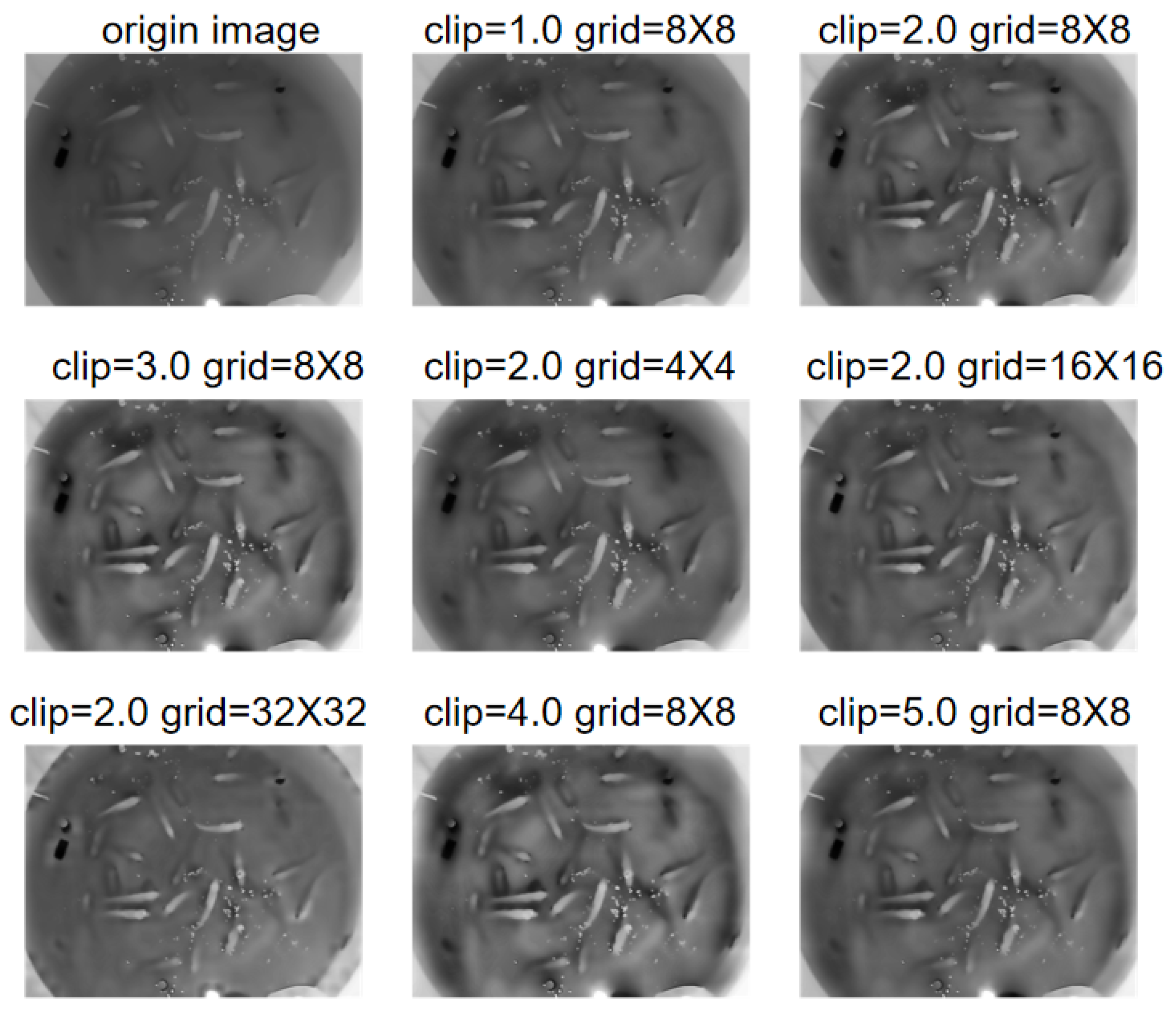The 8 × 8 blocking scheme keeps the artifact rate below 0.8% while maintaining pore texture clarity [29]. We measured images of actual shoals of fish and found that the adult fish presented a long strip shape in 800 × 600 pixel images with a length of about 90 pixels and a width of about 40 pixels. After many trials and comparisons, the final decision was made to divide the image into 8 × 8 small squares. This division has two advantages: first, each square can completely contain 2–3 fish images, and second, one can avoid cutting into the fish body and causing the image to break.

In contrast intensity adjustment, the CLAHE algorithm has an important parameter called clip limit. This parameter controls the strength of the contrast enhancement [30]. We focus on optimizing the control logic of the clip limit parameter, which directly affects the contrast stretch amplitude in local regions of the image. Through a large number of experimental observations, it was found that when the clip limit value is low, the discrimination between the main body of the fish and the water background is insufficient. However, if the parameter is too high, it will lead to abnormal enhancements of noise, such as microscopic particles. To this end, we developed an adaptive adjustment mechanism: Firstly, we analyzed the global gray distribution characteristics of the image and automatically increased the clip limit to 4.0 when significant overlap was detected between the main fish area (gray value mainly distributed in the range of 80–120) and the background water area (gray value concentrated in the range of 60–90). This dynamic adjustment strategy successfully controls the increase in background noise in the ideal range while ensuring the enhancement effect. In order to verify the rationality of the parameter combination, we conducted several groups of control experiments. In the comparison of processing block sizes, although the 4 × 4 block scheme can enhance the texture details of the fish body, it will cause block boundary artifacts. However, the processing of large blocks of 16 × 16 will lead to the blurring of scale features. In the contrast test of clip limit parameter, when the parameter was increased to 5.0, although the fish contour was sharper, the tiny particles such as bait residues would produce over-enhancement artifacts. When the parameter is reduced to 2.0, the edge discrimination between dense fish schools is significantly decreased. After repeated verification, the final 8 × 8 processing block with the clip limit parameter of 4.0 achieved the optimal balance between the fish feature enhancement and the background noise suppression, which not only ensured the clear and sharp edge of the fish body but also controlled the background interference at the visually undetectable level. Figure 2 shows the comparison effect under each parameter combination.

The effect of the dataset before and after processing is shown in Figure 3. As shown in Figure 4, the density level in this study was manually determined based on the number of shallow bright fish in the image. The criteria are as follows: low density: the number of bright fish is less than 3; medium density: 4 to 8 bright fish; high density: the number of bright fish is 9 or more. There are 294 low-density fish school images, 297 medium-density fish school images, and 145 high-density fish school images.

This study addresses the challenge of limited image samples by developing a systematic data augmentation strategy to enhance the model’s generalization capability in complex environments. Based on feature space expansion theory, a multi-modal perturbation mechanism is employed to dynamically reconstruct sample distributions during training. Specifically, input images are first resized to a standardized dimension (adjusted to $\mathrm{IMG}\_\mathrm{SIZE}+32$ pixels) to preserve edge features and spatial distribution information of target objects through an expanded field of view. Subsequently, random cropping is applied (output size: $\mathrm{IMG}\_\mathrm{SIZE}$), generating approximately 1089 spatial variants to effectively simulate potential perspective shifts in real-world monitoring scenarios. For geometric transformations, a multi-axial perturbation strategy is adopted: Random horizontal flipping (probability: 0.5) and vertical flipping (probability: 0.3) enhance model robustness to directional variations, while ±15° random rotation simulates possible angular deviations in equipment installation. To address optical characteristics of aquatic environments, a perspective distortion module (deformation scale: 0.1; application probability: 0.2) is introduced to emulate wave-induced deformation effects. At the spectral enhancement level, leveraging the illumination dynamics of near-infrared imaging, color jittering techniques are applied to independently adjust brightness, contrast, and saturation (perturbation magnitude: 0.3 for each), improving model stability under varying lighting conditions. The core value of this augmentation strategy lies in its systematic expansion of the sample space. Each individual sample can generate approximately 5 distinct variants per epoch on average. This magnitude of feature space reconstruction enables the model to learn more comprehensive sample variation characteristics, particularly for common disturbances in aquatic environments such as scale variations, perspective shifts, and illumination fluctuations. Through real-time streaming processing, this dynamic augmentation solution significantly expands dataset diversity based on limited original data, providing sufficient conditions for the model to learn complex environmental variation patterns while avoiding the storage overhead associated with static dataset expansion.

2.2. Network Model Structure

The deep residual neural network constructed in this paper is based on ResNet-18 [31], which combines the channel attention mechanism with the residual learning paradigm, and it constructs an end-to-end image recognition model with clear layers and powerful feature expression ability. The whole network adopts a phased feature extraction strategy to form a complete calculation flow from the input image to the final classification output. Its core architecture is composed of an input preprocessing module, a multi-level residual feature extraction module, a feature enhancement module, and a classification decision module.

The input image is first processed by a carefully designed initial feature extraction module. This module uses a $7\times 7$ convolution kernel for initial feature extraction. This design has two advantages: On the one hand, a larger receptive field can capture richer spatial context information in the shallow layer of the network, and on the other hand, the initial spatial downsampling is achieved by convolution with a step size of 2. Then, the feature map is standardized through the batch normalization layer to accelerate training convergence and improve the generalization ability of the model, and then, the nonlinear expression ability is introduced through the ReLU activation function. The initial feature map is then entered into a $3\times 3$ Max pooling layer, which further compresses the spatial dimension to 1/4 of the original input while maintaining feature discrimination, forming a 64-channel primary feature representation, which lays a foundation for subsequent deep feature extraction [32].

The feature extraction body adopts a fourth-order progressive residual structure, and each group is composed of two basic residual blocks, forming a channel expansion path from 64 to 128 to 256 to 512. Each basic residual block contains two $3\times 3$ convolution kernels, and batch normalization is implemented after each layer of convolution to ensure the stability of feature distribution. When the size of the input and output feature maps or the channel dimension does not match (mainly occurs in the first layer of each residual block group), the $1\times 1$ convolution kernel is used for spatial downsampling and channel dimension transformation to ensure the accurate alignment of the identity map path and the convolution path. This design allows the deep network to overcome the vanishing gradient problem, which is mathematically expressed as follows:

$$y=F\left(x,\left\{W_i\right\}\right)+W_{s}x$$

(1)

where F represents the residual function, $W_s$ is the projection matrix of dimension matching, and $\left\{W_i\right\}$ represents the set of all learnable parameters in the residual function. The convolution operation with a step size of 2 is used in the first layer of the second to fourth residual block group of the model so that the spatial resolution of the feature map is reduced to $1/8,1/16$, and 1/32 in turn, forming a pyramidal feature abstract structure to capture high-level semantic information on the low-resolution feature map.

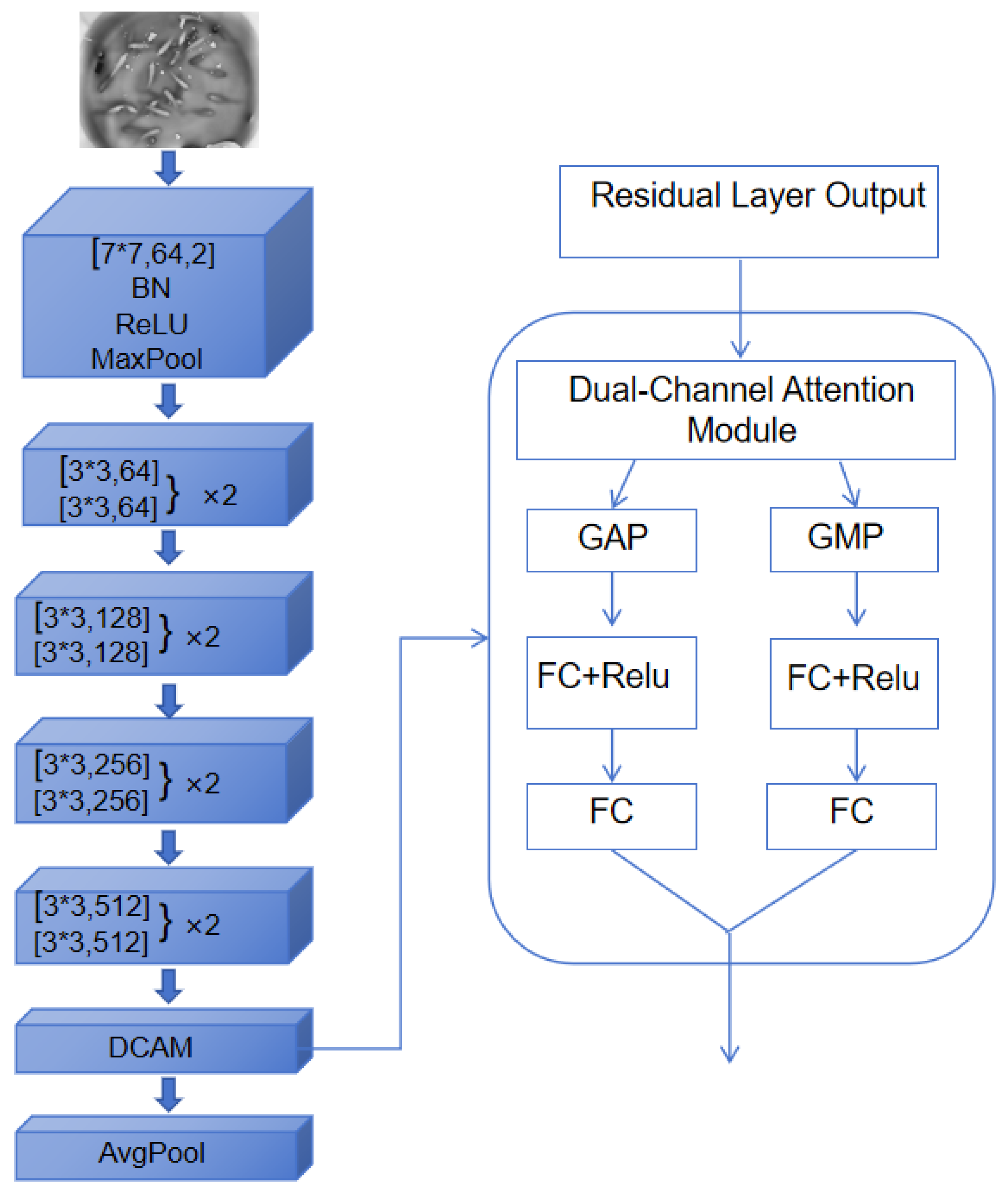
After the fourth residual block group outputs 512 channels of high-level features, a dual-channel attention module (DCAM) is introduced to enhance the feature representation for addressing the unique challenges of near-infrared fish images. The detailed workflow of the DCAM is as follows and is also illustrated in Figure 5.

The input to the DCAM is the feature map $F\in R^{C\times H\times W}$ (where $C=512$). First, the module employs two parallel pooling operations to generate distinct spatial context descriptors: Global Average Pooling (GAP) compresses the feature map into a vector $v_{\mathrm{avg}}\in {\mathbb{R}}^C$ by averaging across spatial dimensions, capturing the global statistical characteristics of the fish school density. Conversely, Global Max Pooling (GMP) generates a vector $v_{\max }\in R^C$ by extracting the maximum activation per channel, which emphasizes locally salient features such as fish boundaries and eyes that are critical in low-contrast NIR images.

The core innovation of the DCAM lies in the subsequent processing of these two descriptors. Instead of using separate fully connected layers, both $v_{\mathrm{avg}}$ and $v_{\max }$ are fed into a shared fully connected bottleneck network. This shared network, denoted as $F_{\mathrm{shared}}(·)$, consists of two linear layers with a reduction ratio of $r=16$. It first projects the input vector from C dimensions down to $C/r$ dimensions, applies ReLU non-linearity, and then projects it back to C dimensions. This parameter-sharing mechanism is mathematically represented as follows:

$$v_{\mathrm{avg}}^{\prime }=F_{\mathrm{shared}}\left(v_{\mathrm{avg}}\right),v_{\max }^{\prime }=F_{\mathrm{shared}}\left(v_{\max }\right)$$

(2)

This design drastically reduces the number of parameters by approximately half compared to a dual-branch structure with independent weights, thereby effectively mitigating the risk of overfitting on small-sample datasets.

The transformed descriptors are then fused through element-wise addition:

$$v_{\mathrm{fused}}=v_{\mathrm{avg}}^{\prime }+v_{\max }^{\prime }$$

(3)

This additive fusion allows the model to adaptively learn the complementary contributions of the global and local features. The fused vector $v_{\mathrm{fused}}$ is passed through a sigmoid function $\sigma (·)$ to generate a channel-wise attention weight vector $w\in {(0,1)}^C$:

$$w=\sigma \left(v_{\mathrm{fused}}\right)$$

(4)

Finally, the original input feature map F is recalibrated by channel-wise multiplication with the attention weights, producing the enhanced feature map $F^{\prime }$:

$$F_c^{\prime }=F_c·w_c,\mathrm{for}\mathrm{each}\mathrm{channel}c$$

(5)

where $w_c$ is the c-th element of w. This operation amplifies the features most relevant to density classification and suppresses less informative ones.

By integrating global and local contextual information through a parameter-efficient, shared-weights architecture, the DCAM significantly improves the model’s robustness and accuracy under challenging imaging conditions.

2.3. Loss Function Design

In this study, the cross-entropy loss function is used as the optimization objective of the model, and its mathematical expression is shown in the following equation:

$$L=-\sum _{i=1}^N{y}_{i}log\left(Y_i\right)$$

(6)

where $y_i$ is the one-hot encoded representation of the true label, and $Y_i$ is the softmax probability predicted by the model. The loss function is designed for multi-classification tasks, which can effectively measure the difference between the predicted probability distribution and the true distribution and optimize the model parameters through the back propagation algorithm.

The optimization algorithm uses the AdamW optimizer, which is a modified version of the Adam optimizer. By decoupling the weight decay and gradient update process, it improves the generalization performance while maintaining the advantages of the adaptive learning rate. The initial learning rate is set to ${10}^{-4}$, and the weight decay coefficient is set to ${10}^{-4}$. These hyperparameters are determined by grid search and show good robustness in several benchmark tasks. Learning rate scheduling adopts the ReduceLROnPlateau strategy, and it uses the validation loss as the monitoring index. When the index does not improve for three consecutive epochs, the learning rate automatically decays to 0.5 times the current one. This adaptive learning rate mechanism can maintain a large update step size in the early stage of training to accelerate convergence, and it automatically reduces the step size to achieve fine-tuning when approaching the optimal point, which significantly improves optimization efficiency.

In order to deal with the problem of class imbalance, this paper introduces the sample weighting mechanism. The WeightedRandomSampler is created by computing the frequency, F_c, of the occurrence of each category in the training set and assigning the category weight w_c = 1/F_c to each sample. This class-based sample reweighting strategy ensures that the model is not biased towards the majority class, which significantly improves the classification performance of the minority class. In the specific implementation, the class distribution C of the complete dataset was counted, and the weight vector w = [1/C0,1/C1,…,1/Ck] was calculated; then, the sample weight Strain was mapped according to the training sample index.

This method improves the sampling probability of minority class samples without changing the actual sample distribution. Early stopping is used to prevent overfitting, and training is stopped when the validation loss does not improve after 10 consecutive epochs. The training monitoring system recorded and visualized the key indicators in real time. The training loss curve and the validation loss curve were distinguished by different colors, and the current indicators were automatically saved to a text file after each epoch. When the validation accuracy reaches a new high, the system automatically saves the current model state, including the model parameters, the current epoch, and the validation accuracy, ensuring that the best model will not be overwritten by subsequent training. This design avoids the uncertainty of manually selecting models while significantly reducing the risk of overfitting. In the process of backpropagation, the gradient dipping strategy is used, and the gradient norm is scaled when it exceeds the threshold of 1.0. This mechanism ensures training stability and, in particular, prevents the gradient explosion problem in deep networks.

3. Experimental Results and Discussion

In the experiments of this paper, the framework of deep learning is PyTorch v2.4.1, the programming language is Python 3.8, and Intel i5 13400f and NVIDIA GeForce RTX 4060 are used for training. During the training process, AdamW is used as the optimizer of the model. Set the learning rate to ${10}^{-4}$, the batch size to 32, the maximum number of iterations (epochs) to 100, and the early stop patience value to 10. The model training parameters are shown in

Table 1. Experimental configuration.

Component	Specification
Graphics Card	NVIDIA GeForce RTX 4060
VRAM	8G
CPU	Intel i5 13400f
Optimizer	AdamW
Max Epochs	100
Learning Rate	${10}^{-4}$
Early Stopping Patience	10
PyTorch Version	2.4.1
CUDA Version	12.4

.

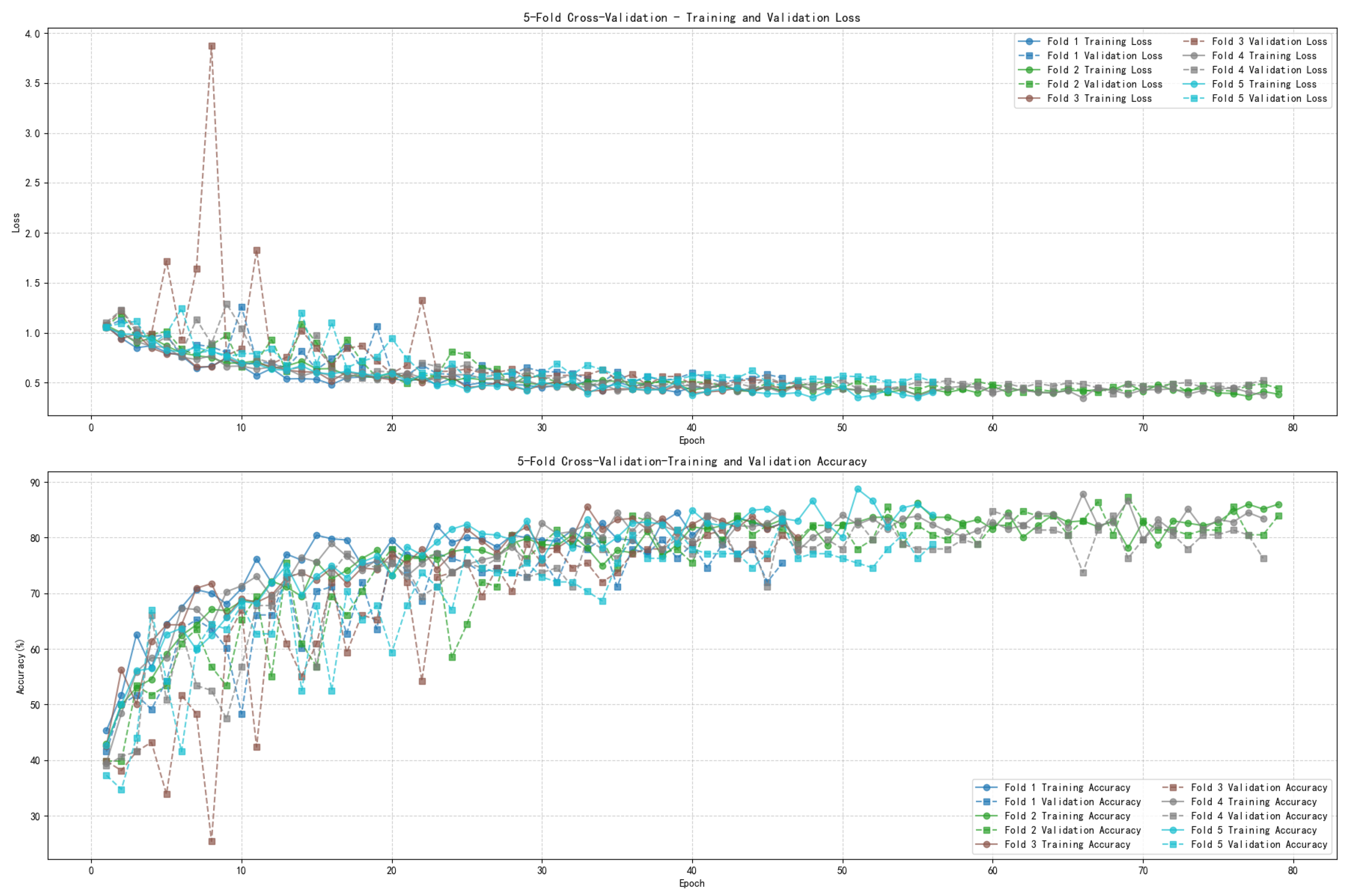
In order to comprehensively evaluate the performance of the model and reduce the impact of random data division, this study adopted a hierarchical five-fold cross-validation strategy [33]: The original dataset was divided into five mutually exclusive subsets, four subsets were used as the training-validation set (further split by 4:2), and the remaining one subset was used as the independent test set. The changes in loss and accuracy of model training are shown in Figure 6, which shows highly robust learning dynamics and stable convergence characteristics: In the initial stage of training (Epoch 0–20), the loss curves of all folds show a significant downward trend, and the training loss and the validation loss decrease simultaneously. The training loss decreases rapidly from the initial high value to the median range, and the validation loss shows a brief abnormal spike at Fold 3 (spiking 150% from the mean value of the same period). However, the fluctuation quickly returned to the baseline decline trajectory within five epochs, and the corresponding verification accuracy quickly rebounded from the valley value of 48% to the normal level. At the same time, the Fold accuracy curves keep rising steadily, with training accuracy steadily increasing from the 40% range to over 75% and validation accuracy climbing from less than 40% to around 65%, with Fold 4 first breaking 80% in the middle stage (around Epoch 30). In the middle and late stage of training (Epoch 20–80), the performance differentiation of each Fold gradually converged. Although Fold 1 showed slight signs of overfitting (the difference between training and validation accuracy was 8%), the overall performance was still within the controllable range. In the final convergence stage (Epoch 60–80), the 50% validation loss is synchronously compressed to a very narrow low value range (0.3–0.4), and the validation accuracy is stable in the range of 80–86%, with Fold 4 leading with 85.8%, and Fold 3 ranking at the bottom with 80.1% affected by the early perturbation. The cross-fold standard deviation is only 2.7%, which indicates that the model has strong adaptability to data partition. Although the training accuracy reaches a high level of 90.3%, it always maintains a reasonable verification gap of 6.5 ± 1.2%, which proves that the regularization mechanism effectively balances the feature memory and generalization ability. To quantitatively assess the statistical significance and robustness of the model’s performance, we conducted a rigorous confidence interval analysis based on the five-fold cross-validation results. The average test accuracy across all folds was 80.57%. Using a paired t-test framework with a 95% confidence level (degrees of freedom = 4; t-critical value ≈ 2.776), the confidence interval was calculated as [78.47%, 82.67%], derived from the individual fold accuracies of [79.73%, 81.63%, 82.99%, 78.91%, and 79.59%]. This narrow interval indicates that the model’s performance is highly reliable and not attributable to random variations in data partitioning. Combined with the low cross-fold standard deviation (2.7%), these results robustly validate the consistency and generalizability of the proposed method under different data splits, effectively addressing potential concerns about statistical fluctuations [34].

In the whole training process, the model verifies the superiority of the architecture design through the triple core capabilities. Firstly, the anti-disturbance recovery ability is demonstrated in the extreme test of Fold 3. The abnormal loss value returns to the baseline efficiently at the rate of 1.16/epoch within four epochs, which highlights the stabilizing effect of the dual-channel attention mechanism on gradient propagation. Secondly, the generalization performance was double verified by the dense distribution (80–86%) and low standard deviation (2.7%) of the cross-fold validation accuracy; in particular, Fold 3 still achieved 80.1% performance, which proved the inclusiveness of the model to noise samples. Thirdly, the effectiveness of the prevention and control of overfitting is reflected in that the training–validation accuracy continues to maintain a reasonable gap of 6.5%, and the 50% validation loss synchronously converges to a steady-state interval of 0.35 ± 0.03, which shows that L2 regularization and the Dropout layer successfully constrain complex feature memory. The efficiency of achieving steady-state convergence within 50 rounds (50% earlier than the preset period) further highlights the optimization potential of the training strategy, which lays an empirical foundation for the application of the lightweight model in complex scenes.

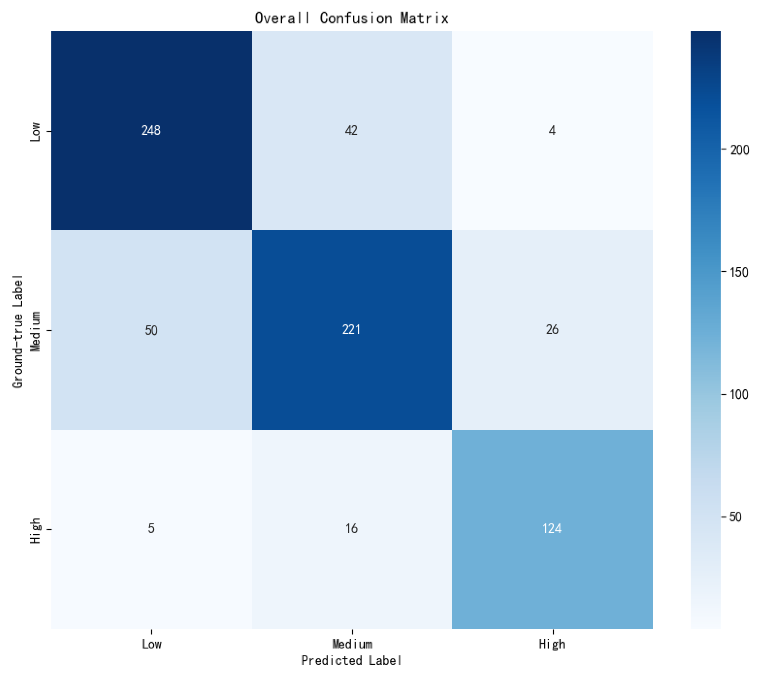
The confusion matrix obtained from the experiment is shown in Figure 7, from which it can be seen that the accuracy of the model is higher when the shallow fish density degree is low, and the accuracy is lower when the shallow fish density degree is medium. There are two main reasons. First, there are many datasets with a low shallow fish density degree, and the model can better learn image features with a low shallow fish density degree, while there are few datasets with a medium shallow fish density degree, and the image features cannot be fully learned. Secondly, the characteristics of fish density in near-infrared images are not obvious, and the bait floating on the water is aggregated into blocks, which increases the interference to the image classification task. The same is true for the low classification accuracy of images with a high clustering degree.

After a comprehensive evaluation of the combined performance of different data processing strategies and model architectures, the proposed improved scheme demonstrates significant advantages while maintaining excellent classification performance and exhibiting commendable computational efficiency. As shown in

Table 2. Model performance comparison.

Model	Recall			F1			Accuracy	Number of Parameters	Inference Time (ms)
	Low	Medium	High	Low	Medium	High
Preprocessed+ MobileNetV3-Small	0.8095	0.6263	0.8828	0.7829	0.6889	0.7901	75.01	1,520,931	25.70
Preprocessed+ ShuffleNet	0.8265	0.7172	0.7379	0.8033	0.7370	0.7405	76.50	1,256,679	23.76
Raw Data+Original ResNet18	0.8644	0.6498	0.7847	0.8199	0.7057	0.7459	76.23	-	-
Raw Data+ResNet18+ DCAM	0.8881	0.6532	0.7917	0.8252	0.7119	0.7808	77.45	-	-
Preprocessed Data+Original ResNet18	0.8095	0.7205	0.8828	0.8054	0.7431	0.8393	78.81	11,178,051	25.70
Preprocessed Data+ResNet18+DCAM	0.8435	0.7441	0.8552	0.8308	0.7674	0.8294	80.57	11,210,819	26.22

, the ResNet18 model with image data preprocessing and dual-channel attention integration achieves the highest accuracy of 80.57% on the test set, which is 4.34 percentage points higher than the ResNet18 baseline model trained on raw data (76.23%). Furthermore, it outperforms the lightweight models ShuffleNet (76.50%) and MobileNetV3-Small (75.01%). In terms of computational efficiency, the improved model has a parameter count of 11.21M and an inference time of 26.22 ms, which remains within the same order of magnitude as the lightweight models (ShuffleNet V2 at 1.26 M/23.76 ms and MobileNetV3-Small at 1.52 M/25.70 ms), highlighting an exceptional balance between accuracy and efficiency. The model also excels in fine-grained classification tasks: In recall metrics, the “medium” density level reaches 0.7441 (a 14.5% improvement over the original ResNet18’s 0.6498), and the “high” level achieves 0.8552 (a 9.0% increase). The F1 score for the “medium” level significantly improves to 0.7674 (compared to only 0.7057 in the original model), validating the enhanced structure’s effectiveness in balanced learning. Ablation studies further reveal that using preprocessed data alone or incorporating only the dual-channel improvement yields inferior results compared to their combined application, indicating that omitting image enhancement or dual-channel attention leads to a decline in fish density recognition rates. It is worth noting that adding an attention module only incurs a minimum overhead of approximately 0.3 M parameters and 0.5 ms inference time, but it helps improve performance and confirms the necessity of each component in addressing the challenges of near-infrared imaging. These optimizations are grounded in a thorough consideration of the physical characteristics of near-infrared imaging. Ultimately, the scheme achieves remarkable accuracy improvements in fish density classification, offering a new technical paradigm for biological monitoring in low-light environments that harmonizes performance and efficiency.

4. Conclusions

In factory aquaculture, it is necessary to use computer vision technology to evaluate the density degree of fish to reduce the workload of manual assessment. At present, most of the assessment of fish feeding intensity based on computer vision technology is carried out in a well-lit environment and lacks consideration of the breeding scene in a dim environment. The use of near-infrared vision technology can realize the observation of fish behavior in dim conditions. However, the low contrast of near-infrared imaging and dynamic illumination fluctuations makes the classification task of fish density extremely challenging. In order to realize the classification task of fish density degree in near-infrared vision, this paper processed original near-infrared image data to enhance the density degree feature of shallow fish and proposed an improved Resnet18 network model to classify the density degree of shallow fish. The proposed model consists of a series of residual blocks, and it uses spatial downsampling and channel dimension transformation to ensure that the identity map path is aligned with the convolution path, which not only enables the deep network to overcome the gradient disappearance problem but also improves the recognition ability of the key features while maintaining high computational efficiency. It provides a feasible solution for complex NIR image classification tasks. The classification accuracy of the improved Resnet18 model is about 4 percentage points higher than that of the original Resnet18 model and nearly 5 percentage points higher than that of the MobileNetV3 model. The F1 score of the three categories of the improved Resnet18 network is higher than that of the original Resnet18 and MobileNetV3.

After improvement, the classification accuracy of Resnet18 reaches 80.57%, which can be basically used in the actual dim farming scene, but its accuracy still has a large room for improvement. The experimental results show that the proposed model has higher classification accuracy for images with a low clustering degree and lower classification accuracy for images with a high clustering degree. This is because the corresponding dataset is very small (only 145, accounting for 19.9%), and high-quality datasets can be added in the future to improve the effect of model learning. In addition, baits floating on the water surface become lumps, which can increase the difficulty for the model to identify the degree of shallow fish density. In this part, some image preprocessing operations can be performed to reduce the influence of decoys on the classification task. Based on the current limitations, we propose the following specific directions for future research: (1) exploring multi-modal data fusion that combines near-infrared imaging with depth information to enhance feature discrimination in complex aquatic environments; (2) optimizing the dynamic adaptability of the attention module to automatically adjust to water quality fluctuations and other complex interference; and (3) establishing a more comprehensive evaluation framework that includes diverse environmental conditions to systematically validate model robustness.