Abstract
Larimichthys polyactis, a key species in East Asian coastal ecosystems, shows distinct seasonal changes in density distribution, shaped by environmental factors and migratory behaviors of two dominant populations (East China Sea and South Yellow Sea). This study explored its 2023 density dynamics in Zhejiang coastal waters using quarterly surveys across 83 stations, combined with generalized additive models (GAM) and random forest (RF) models. Results showed that RF outperformed GAM overall, with bottom dissolved oxygen (SBO), salinity, and depth as the most influential environmental drivers. Density peaked in summer (77.88 thousand ind./km2) in central and northern offshore areas, dominated by the South Yellow Sea population migrating into the region. Autumn densities (3.76 thousand ind./km2) declined sharply as populations moved to overwintering grounds, while spring (0.41 thousand ind./km2) and winter (0.26 thousand ind./km2) densities were lowest. These findings highlight the role of seasonal environmental filters and population-specific migrations in shaping distribution patterns. RF models provide robust tools for predicting habitats, supporting seasonally tailored conservation strategies to protect critical spawning, foraging, and overwintering areas, which are vital for the sustainable management of this ecologically and economically important species.
Keywords:
seasonal biomass density; species distribution models; environmental drivers; Larimichthys polyactis Key Contribution:
We examined seasonal density variations of Larimichthys polyactis in Zhejiang coastal waters using quarterly surveys and species distribution models (GAM and RF), with RF showing superior performance. Our findings reveal that its distinct seasonal density dynamics (peaking in summer, lowest in winter) are highly associated with environmental drivers (bottom dissolved oxygen, salinity, depth) and population-specific migratory behaviors.
1. Introduction
The small yellow croaker (Larimichthys polyactis) is an ecologically and economically vital demersal fish in Northwest Pacific coastal ecosystems, playing a pivotal role in marine food webs as both predator and prey [1,2]. It is an omnivorous fish that feeds on pelagic crustaceans, fish, cephalopods, and other organisms [3]. Its ecological significance is matched by its economic value, supporting fisheries in China and the Republic of Korea, with annual yields exceeding 300,000 tons, making it a critical resource for coastal communities [1,4]. Beyond direct harvest, L. polyactis contributes to ecosystem stability by mediating energy flow between benthic food webs, with its abundance influencing the dynamics of co-occurring species [5].
Over the past four decades, however, L. polyactis populations have experienced severe declines, primarily due to overfishing, habitat degradation from coastal development, and shifts in environmental conditions linked to climate change [6,7]. Historical records indicate a 60% reduction in spawning stock biomass since the 1980s, with particularly sharp declines in the East China Sea [6,8]. These trends have raised concerns about ecological cascades, as reduced L. polyactis abundance may disrupt predator-prey relationships and alter nutrient cycling in coastal waters. Addressing these declines requires a detailed understanding of the species’ habitat requirements, especially how it responds to seasonal environmental changes [9,10].
Seasonal dynamics are a defining feature of marine ecosystems, with temperature, salinity, and productivity fluctuating in response to solar radiation, river discharge, and ocean currents [4]. For migratory species like L. polyactis, these fluctuations drive key life-history events, including spring spawning, summer foraging, autumn migration, and winter overwintering [4,7,11]. For example, spring phytoplankton blooms boost prey availability, supporting energy accumulation for reproduction, while winter temperature drops trigger movements to deeper, thermally stable waters [12]. Yet, despite their importance, seasonal shifts in L. polyactis density have rarely been quantified using rigorous modeling approaches, limiting the precision of conservation strategies [4].
Species distribution models (SDMs) offer a powerful framework to link species occurrence and abundance to environmental factors [13,14]. Traditional models like GAM are well-suited for capturing smooth, non-linear relationships between species and a few environmental factors, such as the effect of depth on fish distribution [15]. Machine learning methods like RF excel at resolving complex interactions between multiple variables, making them valuable for dynamic coastal systems [16]. Comparing these models can reveal not only which environmental factors drive distribution but also how their importance shifts across seasons, a critical insight for adaptive management.
This study aims to fill key gaps in our understanding of L. polyactis ecology by investigating its ecological dynamics in Zhejiang coastal waters. Using quarterly field surveys and SDMs, we analyzed seasonal variations in environmental factors and their impacts on density while evaluating the performance of these models in predicting seasonal distribution patterns. Given the influence of environmental gradients (e.g., depth, salinity) on the species’ life-history strategies, our study seeks to quantify how these variables shape density patterns, identify critical habitats across seasons, and propose seasonally targeted management strategies. This study contributes to advancing knowledge of L. polyactis ecology and underscores the importance of integrating seasonal environmental dynamics into fisheries management. This study can assess the effects of recent conservation measures and provide timely data for policy-making.
2. Materials and Methods
2.1. Study Area
The study was conducted in Zhejiang coastal waters (27°–31° N, 120.5°–123.5° E), a complex marine system encompassing Hangzhou Bay, the Zhoushan Archipelago, and adjacent offshore regions (Figure 1). This area is influenced by three major hydrographic features: the Yangtze River plume, which brings low-salinity water in summer and autumn; the Zhe-Min Coastal Current, a cold, low-salinity current flowing southward; and the Taiwan Warm Current, a warm, high-salinity current intruding northward in winter [6,17,18]. These interactions create strong seasonal gradients in temperature and salinity, with depth ranging from 8 to 10 m in nearshore areas to over 60 m in offshore zones [6].
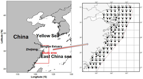
Figure 1.
Study area and survey stations in Zhejiang coastal waters.
2.2. Sampling Design
Surveys were conducted in 2023 across four seasons: spring (April), summer (July), autumn (November), and winter (February), with one cruise per season, totaling 4 surveys. Each cruise covered 83 sampling stations (Figure 1), which were strategically distributed to encompass three distinct habitat types: nearshore (depth < 30 m), mid-shelf (30–50 m), and offshore (>50 m) [10]. This design ensured comprehensive representation of the full environmental gradient in the study area.
Fish sampling used a standardized bottom trawl (net opening circumference 50 m, cod-end mesh size 25 mm) deployed from the research vessel. Each station was trawled for 1 h at a constant speed of 3 knots. To estimate the biomass density of L. polyactis, the swept-area method was applied following the formula for bottom trawl surveys:
where denotes the average resource density in the i-th survey cruise (units: 103 ind./km2 for biomass density); n is the total number of trawl stations in the i-th survey cruise. Cj represents the catch per trawl at the j-th station during the i-th survey cruise. D is the horizontal expansion width of the trawl net mouth. Vj is the average towing speed at the j-th station during the i-th survey cruise. Tj denotes the actual trawling duration at the j-th station during the i-th survey cruise, and E is the escape rate of the catch (set to 0.5 in this study based on the relevant literature on demersal fish escape rates) [19].
Environmental data were collected simultaneously at each station using a Sea-Bird SBE 19plus CTD profiler (Sea-Bird Electronics, Inc., Bellevue, WA, United States), which recorded depth (m); sea surface and bottom temperature (SST, SBT, °C); sea surface and bottom salinity (SSS, SBS, and PSU); sea surface and bottom chlorophyll-a (SSChl, SBChl, mg/m3); and sea surface and bottom dissolved oxygen (SSO, SBO, mg/L). These variables were chosen based on their known influence on L. polyactis physiology and behavior [6,7,8,9].
2.3. Environmental Variable Selection
To avoid multicollinearity, which can bias model results, a variance inflation factor (VIF) analysis was performed on the environmental variables. Variables with VIF >5 were excluded, as they indicated strong correlation with other factors [13]. This process retained eight variables: depth, SBT, SSS, SBS, SSChl, SBChl, SSO, and SBO.
2.4. Model Construction and Evaluation
GAM and RF models were implemented in R (v4.3.2) using the mgcv and randomForest packages, respectively [20,21]. For the GAM, the model formula was specified as follows:
where s( ) denotes a smooth function and by(season) includes interaction terms to account for seasonal differences in species responses to environmental factors.
density ~ s(depth) + s(SBT) + s(SSS) + s(SBS) + s(SSChl) +
s(SBChl) + s(SSO) +s(SBO) + by(season)
For the RF model, 500 decision trees were generated and were sufficient to ensure model stability. Consistent with the GAM, the RF model incorporated the same set of environmental variables and seasonal effects as predictors, ensuring comparability between the two models.
Model performance was evaluated using three metrics: coefficient of determination (R2), mean squared error (MSE), and root mean square error (RMSE) [22]. MSE and RMSE quantified the magnitude of prediction errors (with lower values indicating higher accuracy), while R2 assessed the proportion of variance in density patterns explained by the model (with values closer to 1 indicating stronger explanatory power). Based on these evaluation metrics, the model with superior performance was selected to conduct subsequent predictions of L. polyactis density distribution.
2.5. Spatial Mapping
Predicted density values were interpolated across the study area using ordinary kriging implemented in R (via the gstat package) [23]. This process generated four seasonal predicted distribution maps (one for each survey period), with observed density patterns overlaid directly on the predicted surfaces to visually validate model outputs. The side-by-side comparison of predicted gradients and observed points allowed for qualitative assessment of how well each model captured the spatial structure of L. polyactis density.
3. Results
3.1. Environmental Factor Distribution
Environmental conditions in 2023 exhibited distinct seasonal and spatial heterogeneity, with key variables closely tied to hydrographic processes (Figure 2). SBT ranged from 11.0 ± 1.0 °C in winter to 22.2 ± 3.0 °C in summer. Spatial gradients were striking. In summer, nearshore areas (<30 m) had SBT 2–3 °C higher than offshore zones. By winter, SBT stabilized across depths, varying by <1 °C in offshore regions. Salinity dynamics were dominated by the Yangtze River plume and oceanic currents. SSS dropped to 30.3 ± 1.2 PSU in Autumn, while SBS remained >33 PSU offshore, forming a sharp nearshore-offshore gradient. In summer, a distinct low-salinity zone emerges in the northwestern part of the study area, primarily driven by intensified freshwater input from the Yangtze River plume. This zone exhibits SSS and SBS often below 25 PSU, with a sharp gradient increasing toward the northeastern offshore areas influenced by higher-salinity currents. SSChl and SBChl showed distinct seasonal patterns, with high concentration in summer, medium concentration in autumn and spring, and low concentration in winter, and nearshore areas consistently exceeded offshore zones. SSO showed little seasonal variation across the year, with fluctuations remaining minimal. In contrast, SBO exhibited marked seasonal differences. Spring (7.7 ± 0.8 mg/L) and winter (9.19 ± 0.6 mg/L) levels were significantly higher than those in summer (4.6 ± 1.1 mg/L) and autumn (5.0 ± 1.8 mg/L), reflecting stronger stratification and oxygen consumption in warmer months.
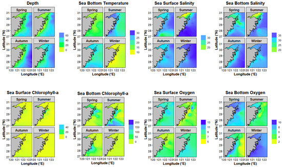
Figure 2.
Environmental conditions in 2023 in Zhejiang coastal waters.
3.2. Model Comparison
Model performance was evaluated using MSE, R2, and RMSE (Figure 3). The results showed that RF achieved the highest R2 value (0.91) among all seasonal comparisons, with a notably stronger fit than GAM in summer. Concurrently, RF exhibited significantly lower MSE and RMSE, indicating more accurate predictions. GAM performed marginally better than RF in spring and winter. Despite GAM’s slight edge in two seasons, RF demonstrated superior overall performance when considering all seasons collectively, especially its stronger predictive power in summer and more consistent error metrics across the year.
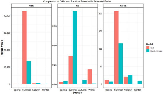
Figure 3.
Comparison of evaluation metrics for GAM and random forest models in different seasons.
We also compared the predicted values of both models against observed data (p > 0.1) (Figure 4). Across spring, autumn, and winter, the discrepancies between predicted and true values were minimal for both models, with no clear distinction in performance. However, in summer, RF predictions aligned significantly closer to observed densities than GAM. Considering all seasons and evaluation metrics, RF demonstrated a stronger overall ability to capture the complexity of L. polyactis density patterns, confirming it as the superior model.
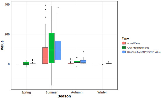
Figure 4.
Comparison of actual and model—predicted values across different seasons. Note: The discrete points in the box plot represent outliers. Outliers > 400 have been deleted in the figure.
3.3. Seasonal Density Distribution of Larimichthys polyactis and Relative Importance of Environmental Factors
L. polyactis density showed clear seasonal shifts (p < 0.05) (Figure 2 and Figure 5). Summer emerged as the season with the highest biomass density across the study area, reaching 77.88 thousand ind./km2, followed by autumn (3.76 thousand ind./km2). In contrast, spring and winter exhibited significantly lower densities, with 0.41 and 0.26 thousand ind./km2, respectively. The bar plot illustrated the relative importance of all eight environmental factors in shaping L. polyactis distribution (Figure 6). Among them, SBO, salinity (both SSS and SBS), and depth consistently showed the highest influence values, underscoring their critical roles in habitat selection across seasons. In contrast, chlorophyll-a (both SSChl and SBChl) exhibited the lowest importance, suggesting that while primary productivity is a background driver, it plays a less important role compared to physical–chemical factors in determining density patterns.
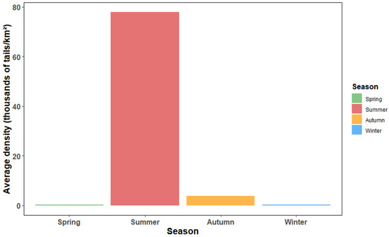
Figure 5.
Seasonal density distribution of Larimichthys polyactis in 2023 in Zhejiang coastal waters.
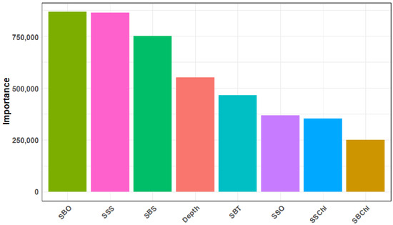
Figure 6.
Relative importance of environmental factors (depth (m), sea bottom temperature (SBT, °C), sea surface salinity (SSS, PSU), sea bottom salinity (SBS, PSU), sea surface chlorophyll-a (SSChl, mg/m3), sea bottom chlorophyll-a (SBChl, mg/m3), sea surface dissolved oxygen (SSO, mg/L), and sea bottom dissolved oxygen (SBO, mg/L) on the density of L. polyactis.
3.4. Predicted Distribution of Larimichthys polyactis
Actual sampling revealed notable differences in L. polyactis occurrence across seasons. Nearly all survey stations captured samples in summer, while only 12 stations recorded the species in winter. We present the predicted distribution patterns based on the RF model (Figure 7). The predicted values of L. polyactis showed good spatial consistency with observed data. Across the study area, offshore deep waters consistently had higher density than nearshore zones, reflecting the species’ preference for more stable deep-water habitats. Seasonal variations in spatial distribution were distinct. In summer, higher biomass density was concentrated in the central and northern regions, with lower values in the south. In spring and autumn, by contrast, southern areas showed higher density. Notably, autumn’s predicted distribution extended beyond the range of actual sampling points, suggesting potential habitats not covered by survey stations. Winter saw minimal density across the entire study area, consistent with the limited number of stations that captured the species during this period.
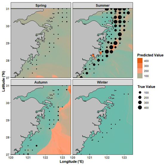
Figure 7.
Potential distribution of Larimichthys polyactis in 2023 in Zhejiang coastal waters. Points represent the survey values, and colors represent the model-predicted values. Notes: the blue color represents the lowest predicted value.
4. Discussion
4.1. Model Performance
In this study, the comparative analysis of GAM and RF models revealed distinct strengths tied to the complexity of environmental relationships in Zhejiang coastal waters. RF consistently outperformed GAM across most seasons, findings that align with observations in Hangzhou Bay [24,25], where RF’s ability to resolve non-linear interactions and threshold effects made it superior for predicting L. polyactis distributions [24]. This superiority was most pronounced in summer, when RF achieved an R2 of 0.91. The strength of RF lies in its ensemble learning framework, which aggregates predictions from multiple decision trees to handle collinearity and interaction effects and is critical in dynamic systems where salinity, temperature, and depth covary [16]. The results reinforce the utility of RF for fisheries management in complex coastal ecosystems, where multi-factor interactions dominate [26,27]. While GAM remains valuable for hypothesis testing—clarifying, for example, that depth has a unimodal effect on density [15]. The predictive power of RF may make it the preferred tool for mapping critical habitats, particularly during ecologically dynamic seasons like summer.
However, RF is not without limitations. Its “black-box” structure obscures the mechanistic links between variables and predictions, making it hard to interpret why certain habitats are preferred [28]. Additionally, it demands greater computational resources, is sensitive to imbalanced sampling data and outliers, and may overfit to noise in small datasets [28]. These limitations also constrain its utility for hypothesis-driven ecological research. Thus, while RF excels at predictive mapping in complex, dynamic systems, GAM remains a powerful tool for refining our understanding of species-environment relationships, particularly when mechanistic insights are prioritized over pure predictive accuracy.
4.2. Environmental Effects for Larimichthys polyactis
The seasonal fluctuations in depth, temperature, salinity, chlorophyll-a, and dissolved oxygen observed in 2023 are not isolated variables but interconnected components of a dynamic “habitat filter” that structures L. polyactis distribution across the year [29]. Among these, SBO, salinity (both SSS and SBS), and depth emerged as the most influential drivers, which were consistent with patterns in coastal ecosystems, where physical stability and physiological constraints dominate habitat selection.
SBO plays a seasonally variable role. The high SBO (9.19 ± 0.6 mg/L) in winter supports overwintering aggregations by ensuring aerobic respiration during reduced feeding, while summer stratification lowers SBO (4.6 ± 1.1 mg/L) in nearshore areas, pushing fish to oxygen-rich offshore zones [11]. Winter’s high bottom dissolved oxygen mitigates hypoxia risks, a growing concern in coastal zones due to eutrophication [30]. Deep-water aggregations during this period are not merely temperature-driven but also reflect a strategy to access oxygen-rich habitats, ensuring aerobic respiration during periods of reduced feeding. This finding aligns with studies of other demersal fishes [31], which prioritize oxygen availability in overwintering habitats to balance energy conservation with survival.
Salinity, shaped primarily by Yangtze River discharge, the Zhe-Min Coastal Current, and the Taiwan Warm Current, acts as a critical filter for larval survival and adult habitat selection [17,18]. Our research results indicated that salinity is the second factor affecting the model. Eggs and larvae of L. polyactis showed higher survival rates in waters with salinity >25 PSU [7], which was aligned with observations in our study. L. polyactis has likely evolved to thrive within specific salinity thresholds that minimize the physiological costs of maintaining internal homeostasis. This adaptation is supported by studies on related species, which have shown that consistent salinity ranges are critical for survival and reproductive success in estuarine and coastal fishes [32,33,34]. Beyond direct physiological effects, shifts in salinity can also alter the distribution and abundance of prey species, such as small crustaceans and planktonic larvae. Therefore, the shifts can reshape the trophic dynamics of the ecosystem and indirectly influence where L. polyactis congregates.
Depth acts as a comprehensive environmental driver, exerting indirect influences on L. polyactis distribution by modulating key factors such as temperature, salinity, and primary productivity. The result of the relative importance of environmental factors indicated depth as the primary determinant of its abundance patterns. Historical studies have shown that L. polyactis species in the East China Sea are concentrated in the water depth range of 40–80 m, with resources less than 60 m deep accounting for 60%, which is consistent with the results of this study [35,36]. Such consistency underscores the adaptive reliance of L. polyactis on mid-to-deep shelf habitats, where depth-mediated stability in temperature and salinity minimizes physiological stress.
Notably, chlorophyll-a (both surface and bottom) had the lowest influence. This pattern may be attributed to the reliance of L. polyactis on mobile prey (e.g., small crustaceans and fish larvae) rather than direct association with phytoplankton [37]. This contrasts with planktivorous species, highlighting the importance of trophic position in shaping environmental dependencies.
4.3. Seasonal Density Patterns and Predicted Distribution
The biomass density of L. polyactis showed striking seasonal shifts that closely tracked the migratory behaviors of the two dominant populations in the region [6,7]. Summer densities, peaking at 77.88 thousand ind./km2 in central and northern offshore areas, were dominated by the South Yellow Sea population, which is consistent with their shorter migratory range and seasonal expansion into the study area. The L. polyactis population completes spawning in the Lvsi Fishing Ground and Haizhou Bay by late spring. These fish move west–southward via the Yellow Sea Warm Current, which transports warmer, nutrient-rich waters into Zhejiang coastal zones. This movement aligns with their preference for summer bottom temperatures (25–27 °C) and mid-to-high salinity (>25 PSU), conditions that optimize foraging efficiency and support the abundance of their primary prey (e.g., small crustaceans and larval fish) [38]. The East China Sea population, though present, plays a secondary role in summer. Post-spawning, a subset of these fish remains in northern nearshore areas off the Zhoushan Archipelago, but their numbers are overshadowed by the larger influx of South Yellow Sea individuals. This overlap creates the observed peak density, with the South Yellow Sea population concentrating in central and northern regions where thermal and salinity gradients best match their physiological tolerances. Notably, the synchrony between South Yellow Sea migration and the seasonal strengthening of the Yellow Sea Warm Current ensures they exploit productive foraging grounds at the optimal time. This timing minimizes competition with the East China Sea population, which tends to occupy shallower, southern habitats during this period. Together, these dynamics underscore the South Yellow Sea population’s role as the primary driver of summer density peaks, with their adaptive movement patterns tightly linked to the region’s hydrographic rhythms. Moreover, there is no significant genetic differentiation between L. polyactis populations in the southern Yellow Sea and East China Sea, but there are phenotypic differences, evidenced by highly significant spatial variations in otolith elemental ratios and otolith morphology [39]. Beyond population movements, survey coverage aligns more closely with the species’ concentrated distribution in summer; summer surveys targeted nursery grounds where juvenile individuals aggregate tightly, directly elevating density estimates. This pattern ultimately reflects the species’ adaptive response to seasonal ecosystem dynamics, prioritizing utilization of summer’s peak productivity.
Spring densities were concentrated in southern nearshore zones, corresponding to spawning aggregations of the East China Sea population. These fish migrate from overwintering grounds southwest of Jeju Island, entering the Zhoushan Fishing Ground by late March to spawn in shallow waters, where stable salinity (>25 PSU) and moderate temperatures (18–20 °C) enhance egg survival [10]. The South Yellow Sea population, meanwhile, begins moving westward from its overwintering grounds to spawn in the Lvsi Fishing Ground, with partial overlap in the northern study area by late spring. Autumn densities declined sharply, and predicted distributions extended beyond sampling ranges. This pattern is explained by pre-overwintering migrations. By November, most East China Sea individuals exit the study area to return to offshore overwintering grounds, while the South Yellow Sea population retreats eastward to its core overwintering zone (123–126° E). This aligns with findings in adjacent regions, where autumn range shifts are linked to pre-overwintering movements [3,6]. Given that predicted autumn distributions extend beyond current sampling boundaries, future studies should expand survey coverage eastward and southward to validate whether the observed density patterns align with model projections, particularly in transitional zones between foraging and overwintering grounds. Winter densities were minimal, with scattered individuals restricted to deep offshore waters. This reflects the East China Sea population’s aggregation in the offshore area of Zhejiang, where stable SBO and temperature support energy conservation, while the South Yellow Sea population remains outside the study area in its distinct overwintering grounds [4].
4.4. Management Implications
The seasonal dynamics and environmental dependencies of L. polyactis highlight the need for targeted management strategies that align with key life-history stages. For spring, protecting spawning grounds in southern nearshore areas through seasonal closures (March–April) would safeguard egg and larval survival, building on the success of Zhejiang’s expanded fishing bans. These areas should be prioritized for no-take zones, as they support the East China Sea population’s reproductive output. Summer requires measures to conserve central and northern offshore foraging grounds, where overlapping populations are most vulnerable to trawling. Restricting bottom trawling in 50–60 m depths during July–September would protect both adult fish and their prey, enhancing growth and energy storage for winter. Autumn management must account for migratory pathways, with expanded monitoring beyond current sampling ranges to track fish moving to overwintering grounds. Coordinating with adjacent regions to limit fishing in these transitional zones (e.g., east of 123° E) could reduce mortality during this critical migration period. Winter calls for the designation of deep-water marine protected areas (MPAs), safeguarding overwintering aggregations of the East China Sea population [40,41]. These MPAs would complement existing protections for the South Yellow Sea population, ensuring both stocks maintain viable spawning biomass.
Finally, adaptive management should integrate model predictions to update habitat maps annually, accounting for interannual variability in river discharge and ocean currents. By aligning conservation with the species’ dynamic habitat needs, these strategies can support the recovery of L. polyactis in Zhejiang coastal waters. The seasonal dynamics identified in this study demand a shift from static to adaptive management, with strategies tailored to the species’ changing habitat needs. Spring’s offshore spawning grounds (east of 122.5° E) are particularly vulnerable, as spawning aggregations are concentrated and highly sensitive to disturbance. Expanding the existing fishing ban to include a no-take zone in these areas from March to April would protect eggs and larvae during their most critical development phase. This aligns with evidence from European MPAs [42].
4.5. Limitations
In this study, our analysis focused on capturing the seasonal variations within the observation year, aiming to reveal key dynamic patterns and driving factors at the seasonal scale. However, we acknowledge that relying solely on one year of data restricts our ability to account for interannual differences; external factors like annual climate fluctuations or interannual changes in anthropogenic activities could alter the studied processes across years, which our current dataset cannot fully reflect. We further propose that future research could integrate multi-year observational data to verify the consistency of the current conclusions and explore long-term evolutionary patterns of the system, which would help improve the generalizability and robustness of the research outcomes. Beyond interannual data constraints, another notable limitation pertains to the unavailability of accurate catch data. Despite recognizing that catch represents the primary human-mediated control on the study population and that its spatial dynamics are essential for evaluating plausible effects on spatial densities, we faced practical barriers in acquiring high-quality catch data. Additionally, the spatial predictions, particularly in unsampled regions, involve a degree of uncertainty due to the inherent smoothing and extrapolation tendencies of kriging. It requires verification through supplementary stations and further study in the future. Moving forward, addressing both interannual data gaps and the lack of accurate catch data would be critical to increasing the rigor of this research area and enhancing the practical relevance of its conclusions for management applications.
5. Conclusions
L. polyactis density in Zhejiang coastal waters exhibits pronounced seasonal shifts, driven by depth, salinity, and temperature, which interact to shape habitat suitability across life-history stages. RF models outperform GAM in capturing these dynamics, offering a robust tool for predicting distribution. Seasonally tailored management for spawning grounds, foraging areas, and overwintering habitats can enhance conservation effectiveness. These findings advance the understanding of L. polyactis ecology and support sustainable management of this ecologically and economically vital species. Moreover, these findings can provide a reference for seasonal conservation strategies of similarly migratory species. Future research should incorporate climate change projections and high-resolution fishing effort data to optimize conservation frameworks amid evolving environmental conditions. Integrating such data with the design of MAPs could further strengthen adaptive management [43,44,45].
Author Contributions
Conceptualization, R.J., K.X. and Y.Z.; methodology, D.W.; data curation, M.H.; writing—original draft preparation, X.L. and P.S.; writing—review and editing, P.S. All authors have read and agreed to the published version of the manuscript.
Funding
This study was supported by the National Key R&D Program (2024YFD2400402), the Fishery Resources Survey Special Program of the Ministry of Agriculture and Rural Affairs (HYS-CZ-202505), and the Zhejiang Fisheries Resources Survey Special Program (HYS-CZ-202502).
Institutional Review Board Statement
This study complies with the Specifications for Oceanographic Surveys Part 6: Marine Biological Surveys and the laws of China. The fish samples were collected with a Bottom trawl net, and the samples were dead when they were obtained. Ethical approval was not required for this study.
Data Availability Statement
Data are unavailable because of institutional access restrictions. Contact the corresponding author for data requests.
Acknowledgments
We thank our colleagues for their contributions to data collection and laboratory experiments. Comments by anonymous reviewers on earlier versions helped improve the manuscript.
Conflicts of Interest
The authors declare no conflicts of interest.
References
- Lin, L.S.; Liu, Z.L.; Jiang, Y.Z.; Huang, W.; Gao, T.X. Current status of small yellow croaker resources in the southern Yellow Sea and the East China Sea. Chin. J. Oceanol. Limnol. 2011, 29, 547–555. [Google Scholar] [CrossRef]
- Zhang, C.; Ye, Z.J.; Wan, R.; Ma, Q.Y.; Li, Z.G. Investigating the population structure of Larimichthys polyactis using otolith features. Fish. Res. 2014, 153, 41–47. [Google Scholar] [CrossRef]
- Lin, L.S. Study on feeding habit and trophic level of redlip croaker in Changjiang estrurary. Mar. Fish. 2007, 29, 44–48. [Google Scholar]
- Xu, M.; Wang, Y.; Liu, Z.; Liu, Y.; Zhang, Y.; Yang, L.; Wang, F.; Wu, H.; Cheng, J. Seasonal distribution of early life stages of L. polyactis adjacent to the Changjiang Estuary. Fish. Oceanogr. 2023, 32, 390–404. [Google Scholar] [CrossRef]
- Tang, Y.; Ma, S.; Liu, C.; Wang, X.; Cheng, S. Environmental influences on L. polyactis in Haizhou Bay. J. Ocean. Univ. China 2018, 17, 973–982. [Google Scholar] [CrossRef]
- Liu, Z.L.; Jin, Y.; Yang, L.L.; Yan, L.P.; Zhang, Y.; Xu, M.; Tang, J.H.; Zhou, Y.D.; Hu, F.; Cheng, J.H. Incorporating egg-transporting pathways into conservation plans of spawning areas: An example of small yellow croaker (Larimichthys polyactis) in the East China Sea zone. Front. Mar. Sci. 2022, 9, 941411. [Google Scholar] [CrossRef]
- Song, X.; Hu, F.; Xu, M.; Zhang, Y.; Jin, Y.; Gao, X.; Liu, Z.; Ling, J.; Li, S.; Cheng, J. Early life stages of L. polyactis in the southern Yellow Sea. Diversity 2024, 16, 521. [Google Scholar] [CrossRef]
- Ding, F.Y.; Lin, L.S.; Li, J.S.; Cheng, J.H. Spawning population of L. polyactis in the northern East China Sea. J. Nat. Resour. 2007, 22, 1013–1019. [Google Scholar]
- Zheng, J.; Gao, T.X.; Yan, Y.R.; Song, N. Genetic variation of L. polyactis from mitochondrial DNA. Acta Oceanol. Sin. 2022, 41, 88–95. [Google Scholar] [CrossRef]
- Yin, J.; Wang, J.; Zhang, C.; Xu, B.; Xue, Y.; Ren, Y.L. L. polyactis egg distribution in Haizhou Bay. J. Fish. Sci. China 2019, 26, 1164–1174. [Google Scholar]
- Parsons, D.F.; Suthers, I.M.; Cruz, D.O.; Smith, J.A. Habitat effects on fish abundance on rocky reefs. Mar. Ecol. Prog. Ser. 2016, 561, 155–171. [Google Scholar] [CrossRef]
- Galaiduk, R.; Radford, B.T.; Saunders, B.J.; Newman, S.J.; Harvey, E.S. Ontogenetic habitat shifts in marine fishes. Ec Appl. 2017, 27, 1776–1788. [Google Scholar] [CrossRef]
- Wan, R.; Song, P.; Li, Z.; Long, X.; Wang, D.; Zhai, L. Use of Ensemble Model for Modeling the Larval Fish Habitats of Different Ecological Guilds in the Yangtze Estuary. Fishes 2023, 8, 209. [Google Scholar] [CrossRef]
- Jin, Z.H.; Xu, K.D.; Zhang, H.L.; Zhou, Y.D.; Long, X.Y.; Zhan, W.; Ma, W.J.; Xu, F. Resource assessment of Sciaenidae fishes in Zhejiang. J. Dalian Fish. Univ. 2025, 40, 156–165. [Google Scholar]
- Murase, H.; Nagashima, H.; Yonezaki, S.; Matsukura, R.; Kitakado, T. GAM application in Sendai Bay fish distribution. ICES J. Mar. Sci. 2009, 66, 1073–1080. [Google Scholar]
- Li, Z.G.; Wan, R.; Ye, Z.J.; Chen, Y.; Ren, Y.P.; Liu, H.; Jiang, Y.Q. Use of random forests and support vector machines to improve annual egg production estimation. Fish. Sci. 2016, 83, 1–11. [Google Scholar] [CrossRef]
- Ren, J.S.; Jin, X.S.; Yang, T.; Kooijman, S.A.L.M.; Shan, X.J. A dynamic energy budget model for small yellow croaker Larimichthys polyactis: Parameterisation and application in its main geographic distribution waters. Ecol. Model. 2020, 427, 109051. [Google Scholar] [CrossRef]
- Zhou, F.; Su, J.L.; Huang, D.J. Coastal low salinity intrusion in the southern Yellow Sea. Haiyang Xuebao 2004, 26, 34–44. [Google Scholar]
- Aglen, A.; Foyn, L.; Godø, O.R.; Myklevoll, S.; Østvedt, O.J. Surveys of the Marine Fish Resources of Peninsular Malaysia, June-July 1980; Institute of Marine Research: Bergen, Norway, 1981; Volume 9, pp. 1–69. [Google Scholar]
- Wood, S.N. Generalized Additive Models: An Introduction with R, 2nd ed.; Chapman & Hall/CRC: Boca Raton, FL, USA, 2017. [Google Scholar]
- Breiman, L. Random forests. Mach. Learn. 2001, 45, 5–32. [Google Scholar] [CrossRef]
- Allouche, O.; Tsoar, A.; Kadmon, R. Assessing species distribution model accuracy. J. Appl. Ecol. 2006, 43, 1223–1232. [Google Scholar] [CrossRef]
- Pebesma, E.J. Multivariable geostatistics in S: The gstat package. Comput. Geosci. 2004, 30, 683–691. [Google Scholar] [CrossRef]
- Long, X.; Wang, D.; Song, P.; Han, M.; Jiang, R.; Zhou, Y. Spatio-Temporal Habitat Dynamics of Migratory Small Yellow Croaker (Larimichthys polyactis) in Hangzhou Bay, China. Fishes 2025, 10, 298. [Google Scholar] [CrossRef]
- Li, M.; Wang, B.; Li, Y. Suspended particulate matters and eutrophication in Hangzhou Bay. Mar. Pollut. Bull. 2024, 207, 116793. [Google Scholar] [CrossRef]
- de la Hoz, C.F.; Ramos, E.; Puente, A.; Juanes, J.A. Temporal transferability of marine distribution models. Ecol. Indic. 2019, 106, 105499. [Google Scholar] [CrossRef]
- Li, Z.G.; Ye, Z.J.; Wan, R.; Zhang, C. Model selection between traditional and popular methods for standardizing catch rates of target species: A case study of Japanese Spanish mackerel in the gillnet fishery. Fish. Res. 2015, 161, 312–319. [Google Scholar] [CrossRef]
- Lee-Yaw, J.A.; McCune, J.L.; Pironon, S. Limitations of species distribution models. Ecography 2022, 45, e05877. [Google Scholar]
- Rubec, P.J.; Santi, C.E.; Ault, J.S.; Monaco, M.E. Modelling estuarine fish distributions. Aquac. Fish Fish. 2023, 3, 1–22. [Google Scholar] [CrossRef]
- Zhou, J.; Hu, H.; Zhu, Z.; Wang, Q.; Li, B.; Hou, S. Dissolved Oxygen Isotopes Unravel Mixing and Respiration Impacts on Coastal Oxygen Depletion Dynamics in the Changjiang Estuary. J. Geophys. Res. Ocean. 2025, 130, e2024JC021474. [Google Scholar] [CrossRef]
- Keller, A.A.; Ciannelli, L.; Wakefield, W.W.; Simon, V.; Barth, J.A.; Pierce, S.D. Species-specific responses of demersal fishes to near-bottom oxygen levels within the California Current large marine ecosystem. Mar. Ecol. Prog. Ser. 2017, 568, 151–173. [Google Scholar] [CrossRef]
- Brunel, T.; van Damme, C.J.G.; Samson, M.; Dickey-Collas, M. Geography and environment in mackerel spawning distribution. Fish. Oceanogr. 2017, 27, 159–173. [Google Scholar] [CrossRef]
- Li, M.; Zhang, C.L.; Xu, B.D. Evaluating the approaches of habitat suitability modelling for whitespotted conger (Conger myriaste). Fish. Res. 2017, 195, 230–237. [Google Scholar] [CrossRef]
- Dambrine, C.; Woillez, M.; Huret, M.; de Pontual, H. Characterising Essential Fish Habitat using spatio-temporal analysis of fishery data: A case study of the European seabass spawning areas. Fish. Oceanogr. 2021, 30, 413–428. [Google Scholar] [CrossRef]
- Zhong, X.M.; Zhang, H.; Tang, J.H.; Zhong, F.; Zhong, J.S.; Xiong, Y.; Gao, Y.S.; Ge, K.K.; Yu, W.W. Temporal and spatial distribution of Larimichthys polyactis Bleeker resources in offshore areas of Jiangsu Province. J. Fish. China 2011, 235, 238–246. [Google Scholar]
- Lin, N.; Chen, Y.G.; Jin, Y.; Yuan, X.W.; Ling, J.Z.; Jiang, Y.Z. Distribution of the early life stages of small yellow croaker in the Yangtze River estuary and adjacent waters. Fish. Sci. 2018, 84, 357–363. [Google Scholar] [CrossRef]
- Akter, S.; Wodeyar, K.A.; Nama, S.; Borah, S.; Angmo, S.; Deshmukhe, G.; Nayak, B.B.; Ramteke, K. Phytoplankton-environment dynamics in a tropical estuary. Environ. Monit. Assess. 2025, 197, 201. [Google Scholar] [CrossRef] [PubMed]
- Wang, Y.L.; Hu, C.L.; Xu, K.D.; Zhou, Y.D.; Jiang, R.J.; Li, Z.H.; Li, X.F. Reproductive status of Larimichthys polyactis in Zhoushan fishing ground and adjacent waters from 2020 to 2021. Ocean Dev. Manag. 2022, 39, 53–57. [Google Scholar]
- Li, Y.; Han, Z.; Song, N.; Gao, T.X. New evidence to genetic analysis of small yellow croaker (Larimichthys polyactis) with continuous distribution in China. Biochem. Syst. Ecol. 2013, 50, 331–338. [Google Scholar] [CrossRef]
- Benedetti-Cecchi, L.; Bertocci, I.; Micheli, F.; Maggi, E.; Fosella, T.; Vaselli, S. Spatial heterogeneity in marine protected areas. Mar. Environ. Res. 2003, 55, 429–458. [Google Scholar] [CrossRef]
- García-Charton, J.A.; Pérez-Ruzafa, A.; Marcos, C.; Claudet, J.; Badalamenti, F.; Benedetti-Cecchi, L.; Falcón, J.M.; Milazzo, M.; Schembri, P.J.; Stobart, B.; et al. Effectiveness of European MPAs. J. Nat. Conserv. 2008, 16, 193–221. [Google Scholar] [CrossRef]
- Roberts, C.M.; Bohnsack, J.A.; Gell, F.; Hawkins, J.P.; Goodridge, R. Effects of marine reserves on adjacent fisheries. Science 2001, 294, 1920–1923. [Google Scholar] [CrossRef]
- Wang, C.L.; Chen, F.; Jiang, R.J.; Zhang, H.L.; Zhu, W.B.; Zhu, K. Effects of typical climate events on spatio-temporal distribution of bottom fish in the coastal waters of Zhejiang. Acta Ecol. Sin. 2024, 44, 4231–4243. [Google Scholar]
- Bento, E.G.; Grilo, T.F.; Nyitrai, D.; Dolbeth, M.; Pardal, M.A.; Martinho, F. Climate influence on juvenile European sea bass (Dicentrarchus labrax, L.) populations in an estuarine nursery: A decadal overview. Mar. Environ. Res. 2016, 122, 93–104. [Google Scholar] [CrossRef] [PubMed]
- Sun, Y.Y.; Zhang, H.; Jiang, K.J.; Xiang, D.L.; Shi, Y.C.; Huang, S.S.; Li, Y.; Han, H.B. Simulating the changes of the habitats suitability of chub mackerel (Scomber japonicus) in the high seas of the North Pacific Ocean using ensemble models under medium to long-term future climate scenarios. Mar. Pollut. Bull. 2024, 207, 12. [Google Scholar] [CrossRef] [PubMed]
Disclaimer/Publisher’s Note: The statements, opinions and data contained in all publications are solely those of the individual author(s) and contributor(s) and not of MDPI and/or the editor(s). MDPI and/or the editor(s) disclaim responsibility for any injury to people or property resulting from any ideas, methods, instructions or products referred to in the content. |
© 2025 by the authors. Licensee MDPI, Basel, Switzerland. This article is an open access article distributed under the terms and conditions of the Creative Commons Attribution (CC BY) license (https://creativecommons.org/licenses/by/4.0/).