
Hardware Implementations of Elliptic Curve Cryptography Using Shift-Sub Based Modular Multiplication Algorithms


Abstract
:1. Introduction
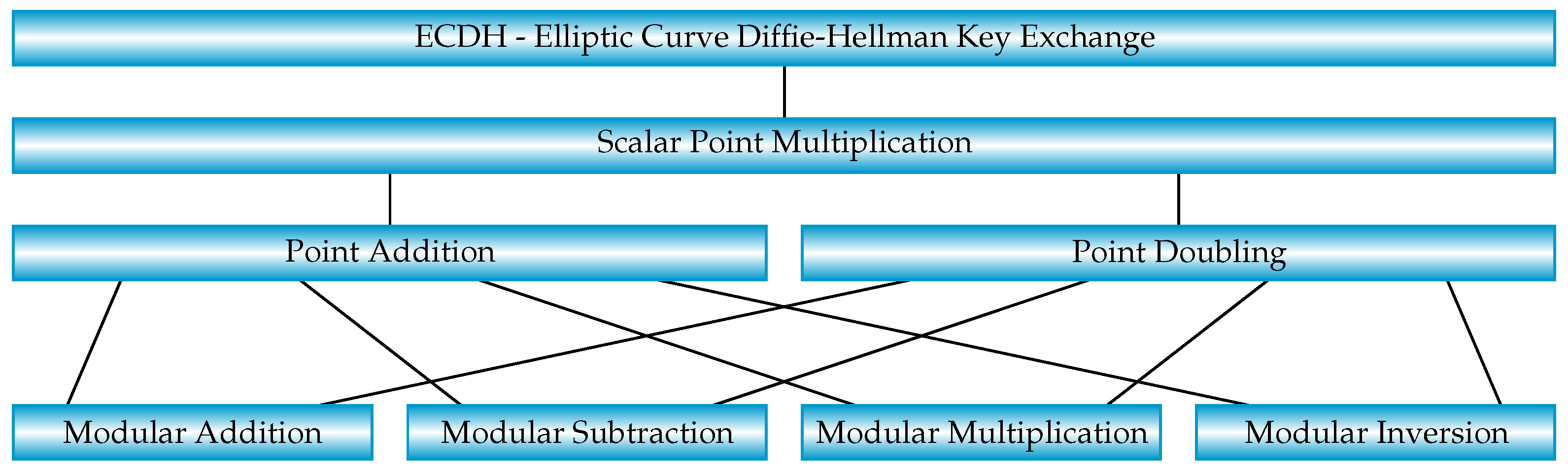
2. Elliptic Curve Cryptography Algorithms
module modadd (a, b, m, s); // s = (a + b) mod m
    input  [255:0] a, b, m;
    output [255:0] s;
    wire   [257:0] sum = {2’b00,a} + {2’b00,b};
    wire   [257:0] s_m = sum - {2’b00,m};
    assign         s   = s_m[257] ? sum[255:0] : s_m[255:0];
endmodule
module modsub (a, b, m, s); // s = (a - b) mod m
    input  [255:0] a, b, m;
    output [255:0] s;
    wire   [257:0] sum = {2’b00,a} - {2’b00,b};
    wire   [257:0] s_m = sum + {2’b00,m};
    assign         s   = sum[257] ? s_m[255:0] : sum[255:0];
endmodule
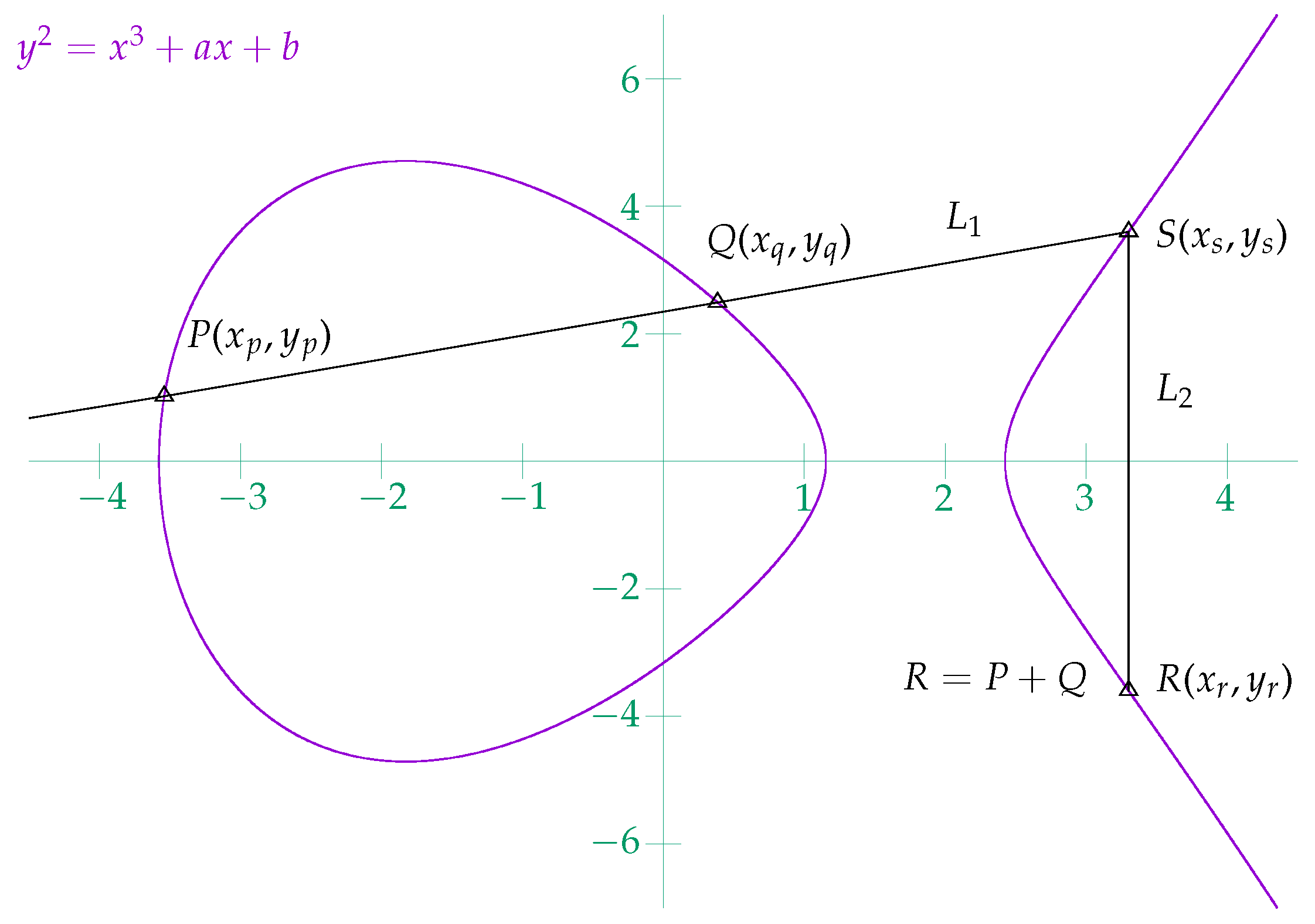
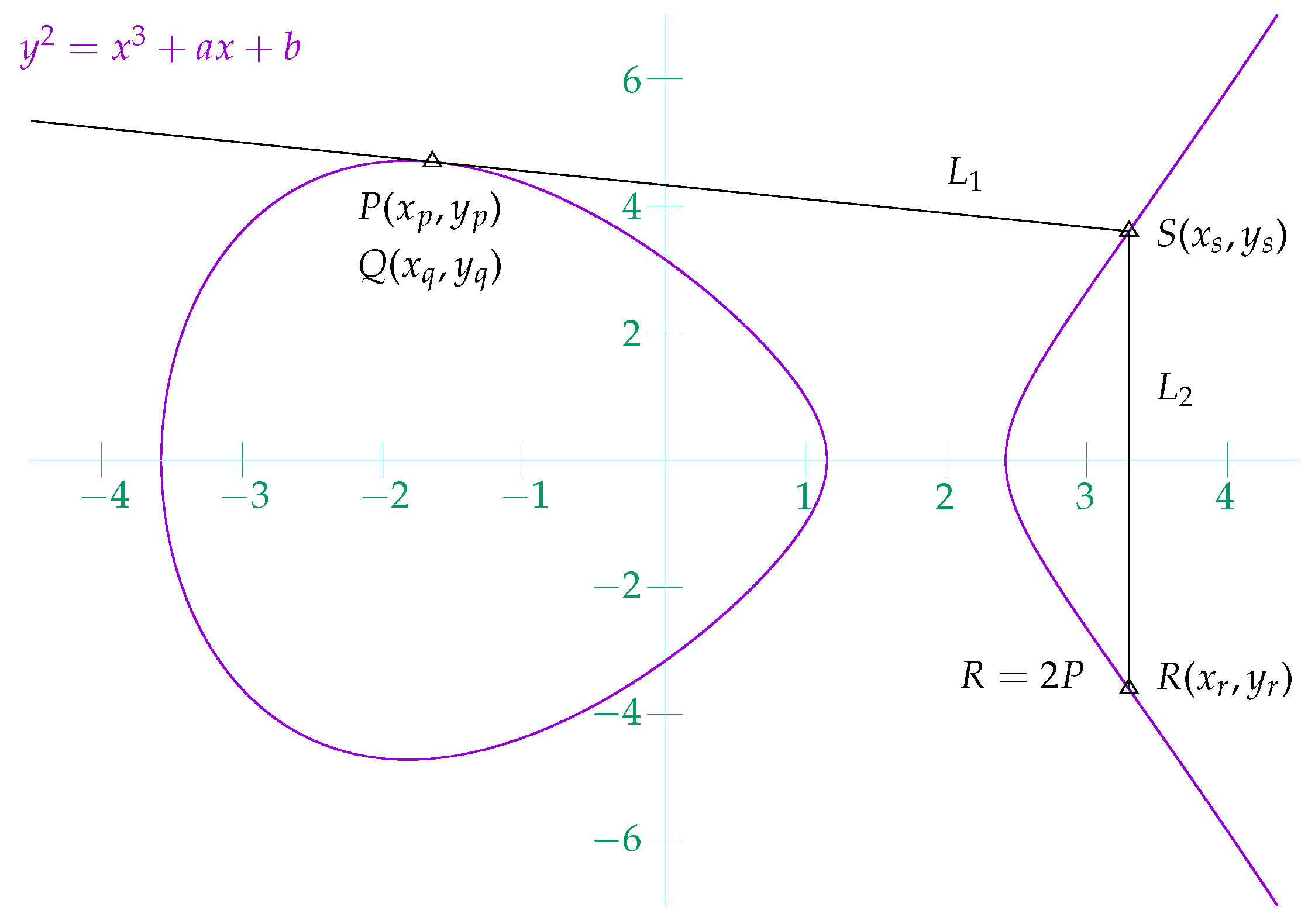
2.1. ECC Point Addition and Doubling in Affine Coordinates
2.1.1. ECC Point Addition in Affine Coordinates
a = 0x0000000000000000000000000000000000000000000000000000000000000000
b = 0x0000000000000000000000000000000000000000000000000000000000000007
m = 0xfffffffffffffffffffffffffffffffffffffffffffffffffffffffefffffc2f
x = 0x79be667ef9dcbbac55a06295ce870b07029bfcdb2dce28d959f2815b16f81798
y = 0x483ada7726a3c4655da4fbfc0e1108a8fd17b448a68554199c47d08ffb10d4b8
| Algorithm 1 PAA (P, Q, m, a) (point addition in affine coordinates). |
|
inputs: Points and ; m and a in
output:
begin
1 , , , ,
2 if return Q /* */
3 if return P /* */
4 if
5 if return O /* */
6 else return PDA () /* */
7
8
9
10 return /* */
end
|
Px = 0xe493dbf1c10d80f3581e4904930b1404cc6c13900ee0758474fa94abe8c4cd13
Py = 0x51ed993ea0d455b75642e2098ea51448d967ae33bfbdfe40cfe97bdc47739922
Qx = 0x79be667ef9dcbbac55a06295ce870b07029bfcdb2dce28d959f2815b16f81798
Qy = 0x483ada7726a3c4655da4fbfc0e1108a8fd17b448a68554199c47d08ffb10d4b8
Rx = 0x2f8bde4d1a07209355b4a7250a5c5128e88b84bddc619ab7cba8d569b240efe4
Ry = 0xd8ac222636e5e3d6d4dba9dda6c9c426f788271bab0d6840dca87d3aa6ac62d6
2.1.2. ECC Point Doubling in Affine Coordinates
| Algorithm 2 PDA (P, m, a) (point doubling in affine coordinates). |
|
inputs: Point ; m and a in
output:
begin
1 , ,
2 if return O /* vertical tangent */
3
4
5
6 return /* */
end
|
Px = 0xb91dc87409c8a6b81e8d1be7f5fc86015cfa42f717d31a27d466bd042e29828d
Py = 0xc35b462fb20bec262308f9d785877752e63d5a68e563e898b4f82f47594680fc
Rx = 0x2d4fca9e0dff8dec3476a677d555896a0980ebccc6bc595a23675496dcc33bb5
Ry = 0xcce413eee9496094256e446b22fd234c03d9258330d77fc8b0d318a6aedba8cb
2.2. ECC Point Addition and Doubling in Projective Coordinates
| Algorithm 3 PAP (P, Q, m, a) (point addition in projective coordinates). |
|
inputs: Points and ; m and a in
output:
begin
1 , , , , , ,
2 if return Q /* */
3 if return P /* */
4 if
5 if return O /* */
6 else return PDP () /* */
7 , , /* level 1 calculations */
8 , /* level 2 calculations */
9 /* level 3 calculations */
10 /* level 3 calculations */
11 /* level 3 calculations */
12 return /* */
end
|
| Algorithm 4 PDP (P, m, a) (point doubling in projective coordinates). |
|
inputs: Point ; m and a in
output:
begin
1 , , ,
2 if return O /* vertical tangent */
3 , /* level 1 calculations */
4 , /* level 2 calculations */
5 /* level 3 calculations */
6 /* level 3 calculations */
7 /* level 3 calculations */
8 return /* */
end
|
Px = 0x61bac660b055382e5906bd6e56e316542194b799b7bcf5ad05ee2171fd81735a
Py = 0xbe44ac0a2b712ccb6bb3ea933e4db0a4213c139078aef594cf8c2c5c2924d54d
Pz = 0x2b6da6fb02877584dc4d5111c88783772d7be5ac2866cce3707d53913384bf49
Qx = 0x6789c1137724f1f3f585337a1814eebc23ea329a0390fd9b1b9ece7af3e71ce1
Qy = 0xc9563c5035ccafec8673f56185141f720073ab3063bb417bf0e70e9d9128c232
Qz = 0x58990cd022b711912676c0451bdab6be04a06c1871b0139214bdbe81fd965555
Rx = 0xf4e9cb9ba9c18876b7b0ad000ce921b35e23139456f4f6c3f70e2fea149500a0
Ry = 0xc06176a9221b6d8b49a22130fb934b21358a1775df68d93ec308aca3ece072b5
Rz = 0x878fb153f0690416ba0ee136ec663debf8472f3ee92d350f9b3a42b4fd53fb27
Px = 0x24fd537e9a5125438a02848f6b74725f678723f5c1450b8fb82a68f0c88c9764
Py = 0xe42e83a1d3d7c2241535b5c0ba5f2462c24bd87aaf9f15b05f3775d168b9bf6c
Pz = 0xe00794d20b32e0e94472c36b89cf5e5d6ec769b53dd6c1422e9467090c272305
Rx = 0x24d00c48ac8bbe61ceb0ac5daf5defd913af9220a07650642a3a41cad9030ee6
Ry = 0x75d429714ea6ce1ab3811d9adc16961a219e2812210fa8465042c18ecd5a0de6
Rz = 0x644a5a2964435364b74d7fa79fe0f06a5b1d2782e7f7b8d1e835db6d6b8786bc
2.3. ECC Point Addition and Doubling in Jacobian Coordinates
Px = 0xe43306185ef298127aef469d577aed78acafaddfc28ad0857491c38ffbedc475
Py = 0x4d83871239769596f65c180546c170a28cffca37bf6393025c457f406f54c517
Pz = 0xdafa620812722dceda7d93a91158dadbe11fee894e71eafa054d5f5fd274377e
Rx = 0x7d7cd6974d7e127a5fdf3f3c9c9eb5dcd9c15e033794466de63bcf2b9548ff85
Ry = 0x8f967b514296945a6dd052bca59ec1418a35cde3c6dd7b269d2e71daa80f851e
Rz = 0xcf89daf8b6c736cc851882b7e85c8ea8f703a9323a3d627909582b7904766035
Px = 0xb7bae589ec8a8c722c1ffb2c37fd4bbeda59074675c3eb50f1673ed46bbedfbe
Py = 0x81dee3398bdd718591c10762f61a0e41c4d609dffddcbeeb3894b8c4ce75e027
Pz = 0x51ec57b21350ad3d3466be5a7d28742279fbac1146fb4143767ee368a7dc741e
Qx = 0x0aa20a04dba4788e9b99e10f2e9f4d43b7f53916a5cacf2050dc70bc34c18d21
Qy = 0x60f318d01180b303f4b20a49c2b7e2b498405f88bd423a9a7cb92bab5f1b6abf
Qz = 0x3e1dcb6efa88b113f40b5858ea8c3cb5ddae2277c4683af9487e27023cba690d
Rx = 0x348248c47ad5d3186bd807c382659263840ba7ea13e61128d24337db9b0e5278
Ry = 0xb38573698dd6fef9ec93a9d68ae0a997191b678474cc00a13961defa3ed763e9
Rz = 0x76da2008046aae9901e6b96a7b54c42fd480de5cbc8cef6c0d0a9b3d7086f0f4
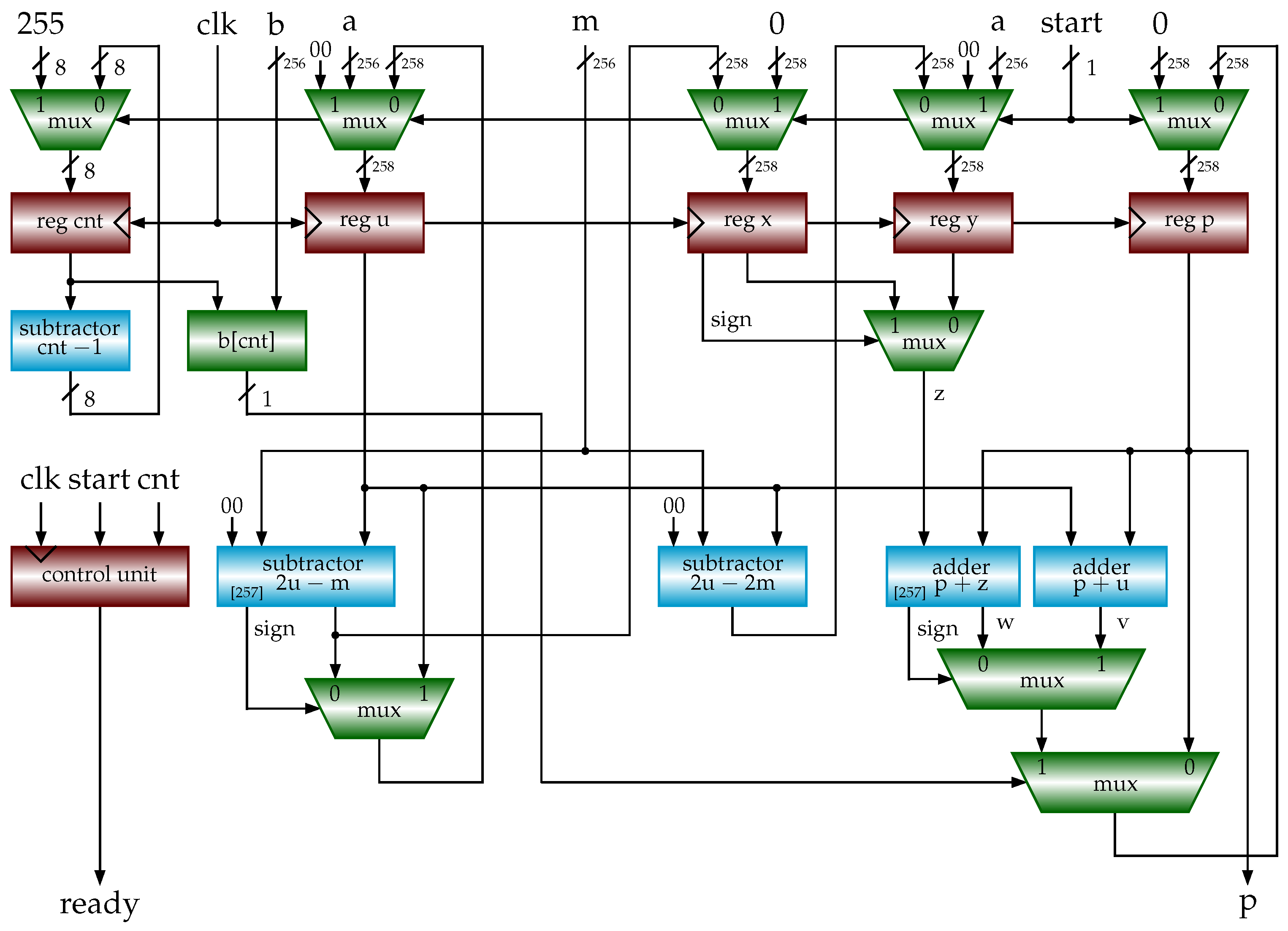
2.4. Modular Inversion
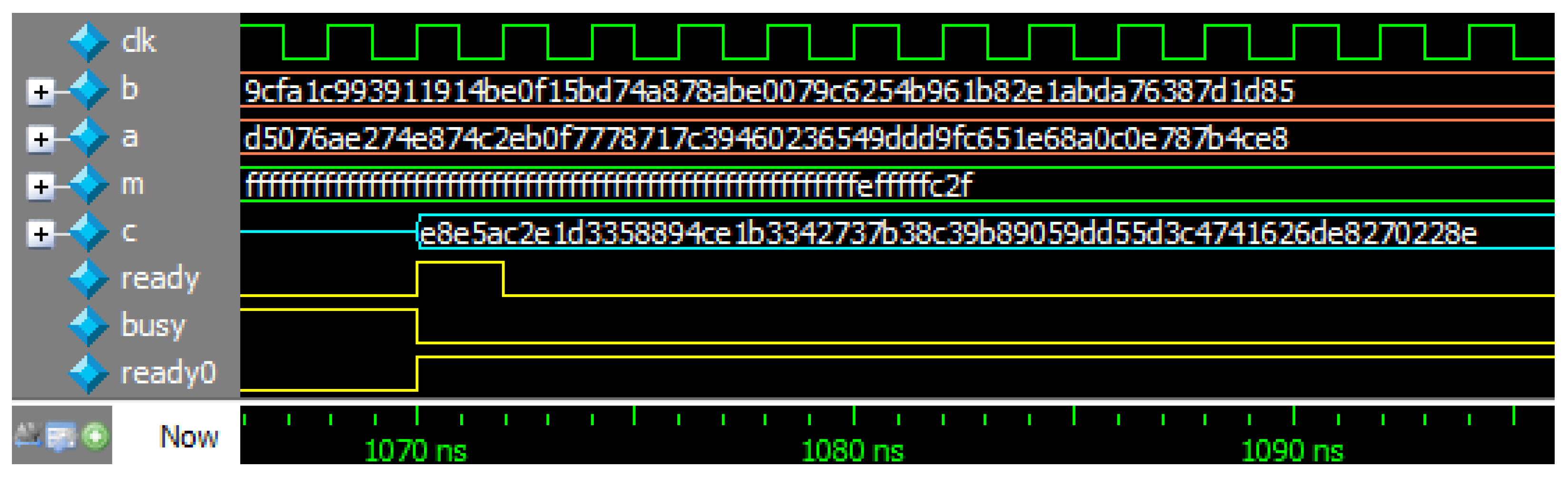
b = 0x9cfa1c993911914be0f15bd74a878abe0079c6254b961b82e1abda76387d1d85
a = 0xd5076ae274e874c2eb0f7778717c39460236549ddd9fc651e68a0c0e787b4ce8
m = 0xfffffffffffffffffffffffffffffffffffffffffffffffffffffffefffffc2f
c = 0xe8e5ac2e1d3358894ce1b3342737b38c39b89059dd55d3c4741626de8270228e
2.5. Scalar Point Multiplication
| Algorithm 5 ScaMul (d, P, m, a) (scalar point multiplication). |
|
inputs: and point ; m and a in
output:
begin
1 , , /* and */
2 while to
3 if
4 /* point addition */
5 /* point doubling */
6
7 endwhile
8 return Q /* */
end
|
| Weight | Point Addition | Point Doubling | |
| Initial | |||
| 1 | |||
| 2 | |||
| 4 | |||
| 8 | |||
| 16 |
2.6. Elliptic Curve Diffie–Hellman Key Exchange
-
Alice generates and exposes :
da   = 0x650aa7095daeaa37ab9051541f0ce304f8969a6d88bb3bebb4fe680fca9a2595
Qax  = 0x167d2537aa6bbd8d978b58be0f9466520b7b184e205ff96a9ff567b35b32c7b7
Qay  = 0xde3961553d36551f92726fee0e332133960edddccd2784b98b2af730d2fc6e14
-
Bob generates and exposes :
db   = 0xedc68f194c4e30d6ef90467df822b00e5ef122dea48c9d1c54817080d1a341f4
Qbx  = 0x839da64a414c2243a5526230603109be9c615613a9e98c3d650bb0488580bbda
Qby  = 0x96e88e99304a5afcdd77c4f3b3327a28162627ebe08194baa0c78dfb67a11042
-
Alice obtains and calculates :
Qabx = 0x1f254c7da15899275cdcab9d992f58251a4ab630fe9864d20cf317ab57749947
Qaby = 0xd6cb400b3c49d33d3df28f9d34fa09f8b6c8edf117a378c5a45d0a51e6c0debc
-
Bob obtains and calculates :
Qbax = 0x1f254c7da15899275cdcab9d992f58251a4ab630fe9864d20cf317ab57749947
Qbay = 0xd6cb400b3c49d33d3df28f9d34fa09f8b6c8edf117a378c5a45d0a51e6c0debc
-
Now, Alice and Bob have a same secret key (). They can use a symmetric-key cryptography for the subsequent communications.
3. Modular Multiplication Algorithms
3.1. Interleaved Modular Multiplication Algorithm
| Algorithm 6 IMM (a, b, m) (interleaved modular multiplication). |
inputs: , , , m: n-bit odd number output: begin 1 /* product */ 2 for downto 0 3 /* */ 4 /* add multiplicand a to p if */ 5 if , /* subtract m from p */ 6 if , /* subtract m from p */ 7 return p end |
3.2. Montgomery Modular Multiplication Algorithm
| Algorithm 7 MMM (a, b, m) (Montgomery modular multiplication). |
inputs: , , , , m: n-bit odd number output: begin 1 /* product */ 2 for to 3 /* add multiplicand a to p if */ 4 /* make p even */ 5 /* : reduction */ 6 if , /* subtract m from p in the finalization */ 7 return p end |
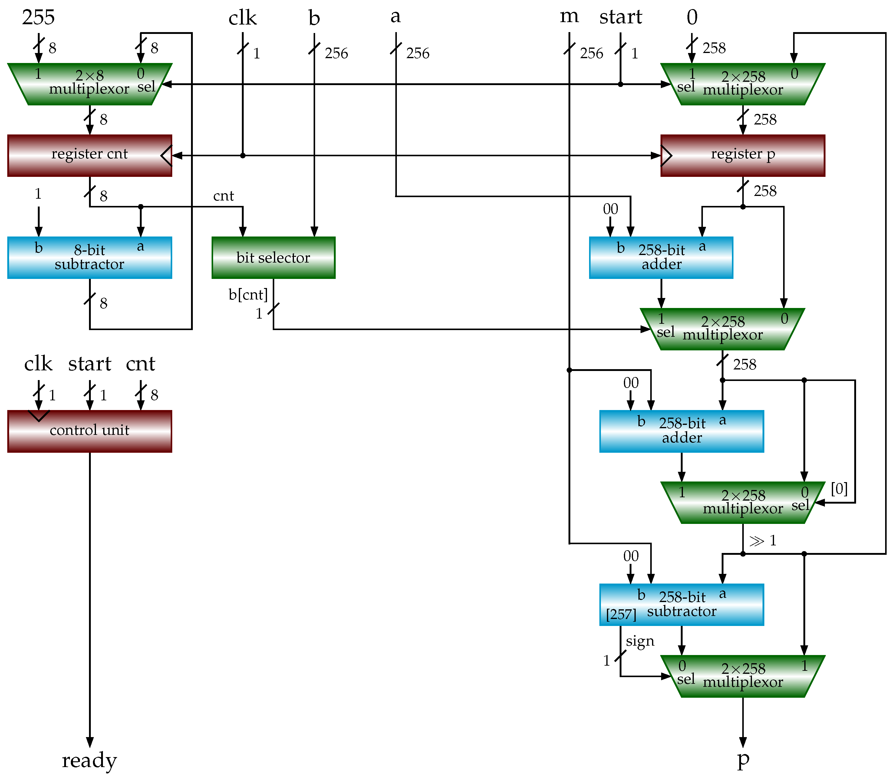
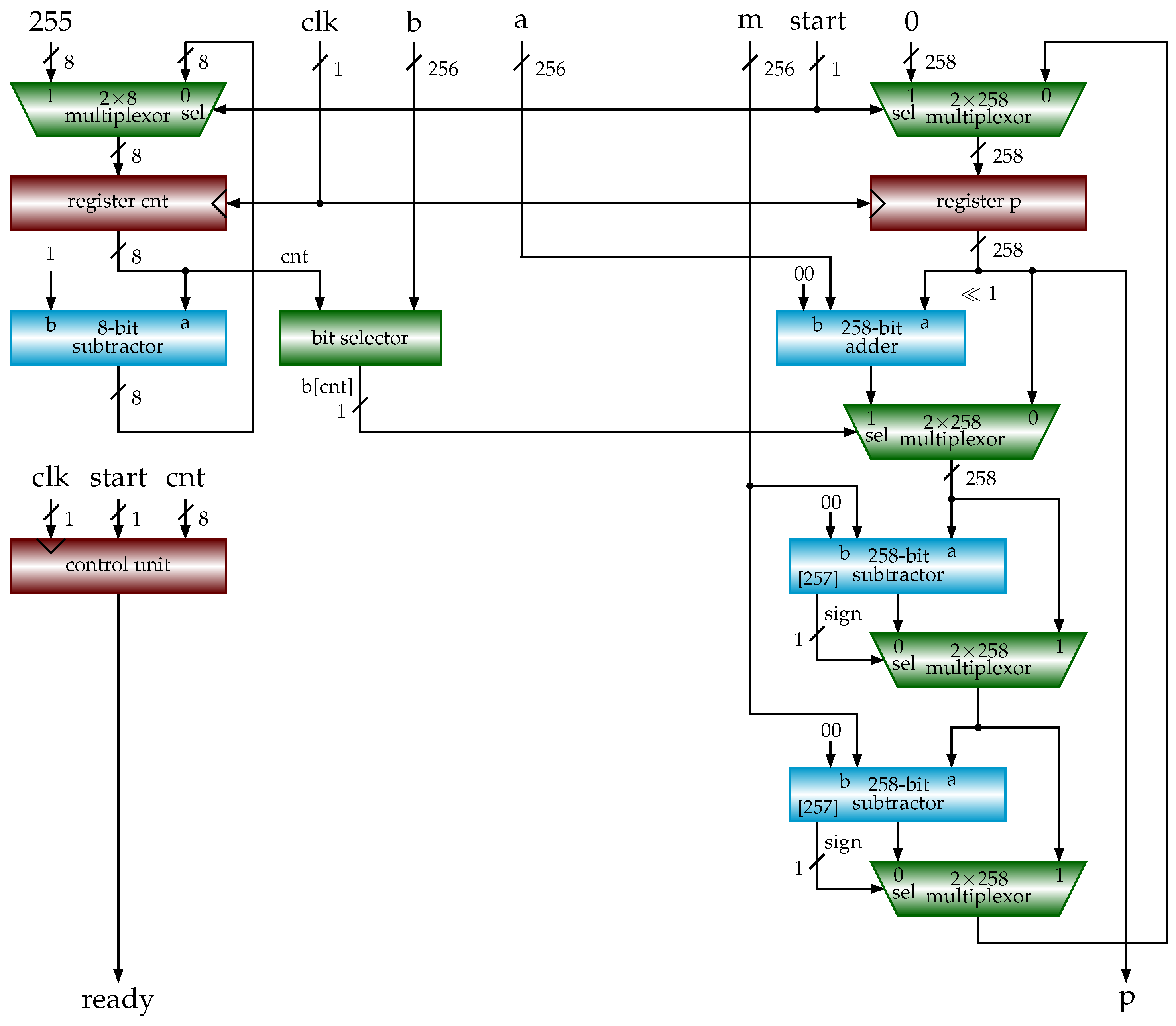
3.3. Shift-Sub Modular Multiplication Algorithm
| Algorithm 8 SSMM (a, b, m) (shift-sub modular multiplication). |
inputs: , , , m: n-bit odd number output: begin 1 ; /* multiplicand, product */ 2 for to 3 /* add multiplicand u to p if */ 4 if , /* subtract m from p */ 5 6 if , /* subtract m from u */ 7 return p end |
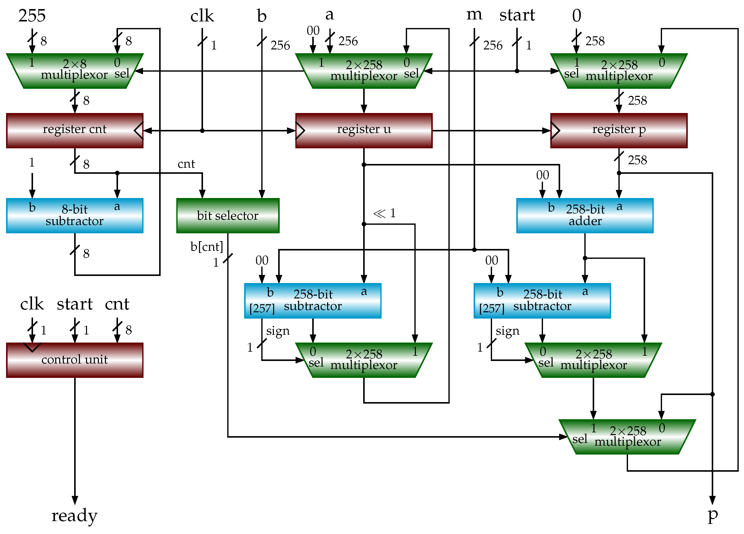
3.4. Shift-Sub Modular Multiplication with Advance Preparation Algorithm
| Algorithm 9 SSMMPRE (a, b, m) (shift-sub modular multiplication with preparation). |
inputs: , , , m: n-bit odd number output: begin 1 ; ; ; 2 for to 3 4 if , /* x: prepared in previous clock cycle */ 5 else /* y: prepared in previous clock cycle */ 6 if 7 if , 8 else 9 ; /* prepare for use in next clock cycle */ 10 if , 11 else 12 return p end |
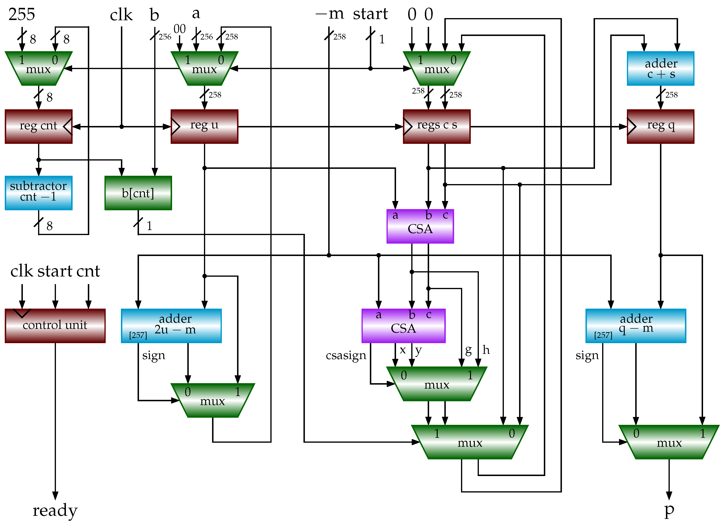
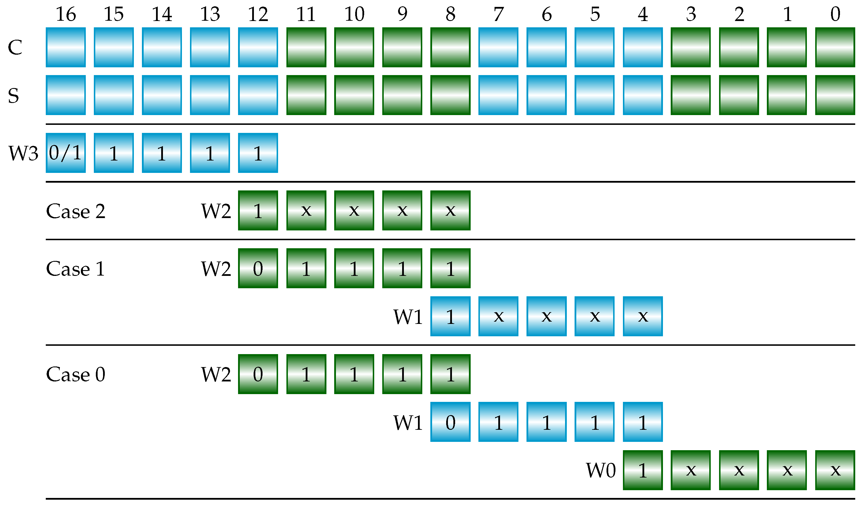
3.5. Shift-Sub Modular Multiplication with CSAs and Sign Detection Algorithm
| Algorithm 10 SSMMCSA (a, b, m) (shift-sub modular multiplication with CSAs). |
inputs: , , , m: n-bit odd number output: begin 1 ; 2 for to 3 4 if 5 /* add multiplicand u to */ 6 7 if sign (negative) 8 9 else /* subtract m from */ 10 11 if 12 /* subtract m from u */ 13 if 14 /* subtract m from q */ 15 return p end |

| = | + | (Add 5-bit, 5-bit sum) | ||||
| = | + | (Add 4-bit, 5-bit sum) | ||||
| = | + | (Add 4-bit, 5-bit sum) | ||||
| = | + | (Add 4-bit, 5-bit sum) |

| sign_inverse | = | Case 2 | ||||||
| | | ’b | & | Case 1 | |||||
| | | ’b | & | ’b | & | Case 0 |
4. Hardware Implementations of Modular Multiplications and ECC
4.1. Hardware Implementations of Modular Multiplications
4.2. Hardware Implementations of ECC
module scalarmult (clk, rst_n, start, x, y, d, m, a, rx, ry, ready);
	// … signal declarations
	addpoints ap (clk, rst_n, start_ap, x1, y1, x2, y2, m, a, apx, apy, ready_ap);
	doublepoint dp (clk, rst_n, start_dp, x1, y1, m, a, dpx, dpy, ready_dp);
	always @(posedge clk or negedge rst_n) begin
		// … to generate start_ap and start_dp and register results
		// … to check completeness and generate signals for ready
	end
endmodule
    if r - 2m >= 0
       c = r - 2m          // c = r - 2m
    else if r - m >= 0
            c = r - m      // c = r - 1m
         else if r >= 0
                 c = r     // c = r + 0m
              else
                 c = r + m // c = r + 1m
              endif
         endif
    endif
5. Conclusions and Future Work
Funding
Data Availability Statement
Conflicts of Interest
Appendix A. Verilog HDL Code of Shift-Sub Modular Multiplication (SSMM)
‘timescale 1ns/1ns
module modmul (clk, rst_n, start, a, b, m, p, ready, busy, ready0);            // p = a * b mod m
    input          clk, rst_n;
    input          start;
    input  [255:0] a, b, m;
    output [255:0] p;
    output         ready;
    output reg     busy;
    output reg     ready0;
    reg            ready1;
    assign ready = ready0 ^ ready1;
    reg    [257:0] u, s;
    reg      [7:0] cnt;
    wire     [7:0] next_cnt = cnt + 8’d1;
    wire           bi_is_1  = b[cnt];
    wire   [257:0] plus_u   = s + u;                                           // s + u
    wire   [257:0] minus_m  = plus_u - {2’b00,m};                             // s + u - m
    wire   [257:0] new_s    = bi_is_1 ? minus_m[257] ? plus_u : minus_m : s;   // new s
    wire   [257:0] two_u    = {u[256:0],1’b0};                                // 2u
    wire   [257:0] two_u_m  = two_u - {2’b00,m};                              // 2u - m
    wire   [257:0] new_u    = two_u_m[257] ? two_u : two_u_m;                  // new u
    assign p = s[255:0];
    always @(posedge clk or negedge rst_n) begin
        if (!rst_n) begin
            ready0 <= 0;
            ready1 <= 0;
            busy   <= 0;
        end else begin
            ready1 <= ready0;
            if (start) begin
                u <= {2’b0,a};                                                // u <= a
                s      <= 0;                                                   // s <= 0
                ready0 <= 0;
                ready1 <= 0;
                busy   <= 1;
                cnt    <= 0;
            end else begin
                if (busy) begin
                    s <= new_s;                                                // s <= new_s;
                    if (cnt == 8’d255) begin                                  // finished
                        ready0 <= 1;
                        busy   <= 0;
                    end else begin                                             // not finished
                        u   <= new_u;                                          // u <= new_u;
                        cnt <= next_cnt;                                       // cnt++
                    end
                end
            end
        end
    end
endmodule

Appendix B. Verilog HDL Code of Modular Inversion
‘timescale 1ns/1ns
module modinv (clk, rst_n, start, b, a, m, c, ready, busy, ready0);            // c = b * a^{-1} mod m
    input          clk, rst_n;
    input          start;
    input  [255:0] b, a, m;
    output [255:0] c;
    output         ready, ready0;
    output reg     busy;
    reg            ready0,  ready1;
    assign ready = ready0 ^ ready1;
    reg    [259:0] u, v, x, y, q, result;
    wire   [259:0] x_plus_m   = x + q;                                         // x + m
    wire   [259:0] y_plus_m   = y + q;                                         // y + m
    wire   [259:0] u_minus_v  = u - v;                                         // u - v
    wire   [259:0] r_plus_m   = result + q;                                    // r + m
    wire   [259:0] r_minus_m  = result - q;                                    // r - m
    wire   [259:0] r_minus_2m = result - {q[258:0],1’b0};                     // r - 2m
    assign c = r_minus_2m[259] ? r_minus_m[259] ? result[259] ? r_plus_m[255:0] :
               result[255:0] : r_minus_m[255:0] : r_minus_2m[255:0];           // c = b * a^{-1} mod m
    always @(posedge clk or negedge rst_n) begin
        if (!rst_n) begin
            ready0 <= 0;
            ready1 <= 0;
            busy   <= 0;
        end else begin
            ready1 <= ready0;
            if (start) begin
                u <= {4’b0,a};                                                 // u <= a
                v <= {4’b0,m};                                                 // v <= m
                x <= {4’b0,b};                                                 // x <= b
                y <= {260’b0};                                                 // y <= 0
                q <= {4’b0,m};                                                 // q <= m
                ready0 <= 0;
                ready1 <= 0;
                busy   <= 1;
            end else begin
                if (busy && ((u == 1) || (v == 1))) begin                       // finished
                    ready0 <= 1;
                    busy   <= 0;
                    if (u == 1) begin                                           // if u == 1
                        if (x[259]) begin                                       //     if x < 0
                            result <= x_plus_m;                                 //         c = x + m
                        end else begin                                          //     else
                            result <= x;                                        //         c = x
                        end
                    end else begin                                              // else
                        if (y[259]) begin                                       //     if y < 0
                            result <= y_plus_m;                                 //         c = y + m
                        end else begin                                          //     else
                            result <= y;                                        //         c = y
                        end
                    end
                end else begin                                                  // not finished
                    if (!u[0]) begin                                            // while u & 1 == 0
                        u <= {u[259],u[259:1]};                                 //     u = u >> 1
                        if (!x[0]) begin                                        //     if x & 1 == 0
                            x <= {x[259],x[259:1]};                             //         x = x >> 1
                        end else begin                                          //     else
                            x <= {x_plus_m[259],x_plus_m[259:1]};               //         x = (x + m) >> 1
                        end
                    end
                    if (!v[0]) begin                                            // while v & 1 == 0
                        v <= {v[259],v[259:1]};                                 //     v = v >> 1
                        if (!y[0]) begin                                        //     if y & 1 == 0
                            y <= {y[259],y[259:1]};                             //         y = y >> 1
                        end else begin                                          //     else
                            y <= {y_plus_m[259],y_plus_m[259:1]};               //         y = (y + m) >> 1
                        end
                    end
                    if ((u[0]) && (v[0])) begin                                 // two while loops finished
                        if (u_minus_v[259]) begin                               // if u < v
                            v <= v - u;                                         //     v = v - u
                            y <= y - x;                                         //     y = y - x
                        end else begin                                          // else
                            u <= u - v;                                         //     u = u - v
                            x <= x - y;                                         //     x = x - y
                        end
                    end
                end
            end
        end
    end
endmodule
‘timescale 1ns/1ns
module modinv_tb;
    reg          clk, rst_n, start;
    reg  [255:0] b, a, m;
    wire [255:0] c;
    wire         ready, busy, ready0;
    modinv inst (clk, rst_n, start, b, a, m, c, ready, busy, ready0);
    initial begin
        #0 clk   = 1;
        #0 rst_n = 0;
        #0 start = 0;
        #0 b     = 256’h9cfa1c993911914be0f15bd74a878abe0079c6254b961b82e1abda76387d1d85;
        #0 a     = 256’hd5076ae274e874c2eb0f7778717c39460236549ddd9fc651e68a0c0e787b4ce8;
        #0 m     = 256’hfffffffffffffffffffffffffffffffffffffffffffffffffffffffefffffc2f;
        #1 rst_n = 1;
        #2 start = 1;
        #2 start = 0;
        wait(ready);
        #40 $stop;
    end
    always #1 clk = !clk;
endmodule

References
- Koblitz, N. Elliptic curve cryptosystems. Math. Comput. 1987, 48, 203–209. Available online: https://www.ams.org/journals/mcom/1987-48-177/S0025-5718-1987-0866109-5/S0025-5718-1987-0866109-5.pdf (accessed on 15 October 2023). [CrossRef]
- Miller, V.S. Use of Elliptic Curves in Cryptography. In Proceedings of the Advances in Cryptology—CRYPTO’85 Proceedings; Springer: Berlin/Heidelberg, Germany, 1986; pp. 417–426. Available online: https://link.springer.com/content/pdf/10.1007/3-540-39799-X_31.pdf?pdf=inline%20link (accessed on 15 October 2023).
- Hankerson, D.; Menezes, A.; Vanstone, S. Guide to Elliptic Curve Cryptography; Springer: New York, NY, USA, 2004. [Google Scholar] [CrossRef]
- Certicom_Corp. Standards for Efficient Cryptography. SEC 2: Recommended Elliptic Curve Domain Parameters; Certicom Corp: Mississauga, ON, Canada, 2010; Available online: http://www.secg.org/sec2-v2.pdf (accessed on 15 October 2023).
- Barker, E.; Chen, L.; Roginsky, A.; Vassilev, A.; Davis, R. SP 800-56A Rev. 3, Recommendation for Pair-Wise Key-Establishment Schemes Using Discrete Logarithm Cryptography; National Institute of Standards and Technology: Gaithersburg, MD, USA, 2018. Available online: https://nvlpubs.nist.gov/nistpubs/SpecialPublications/NIST.SP.800-56Ar3.pdf (accessed on 15 October 2023).
- Blakely, G.R. A Computer Algorithm for Calculating the Product AB Modulo M. IEEE Trans. Comput. 1983, C-32, 497–500. [Google Scholar] [CrossRef]
- Islam, M.M.; Hossain, M.S.; Hasan, M.K.; Shahjalal, M.; Jang, Y.M. FPGA Implementation of High-Speed Area-Efficient Processor for Elliptic Curve Point Multiplication over Prime Field. IEEE Access 2019, 7, 178811–178826. [Google Scholar] [CrossRef]
- Islam, M.M.; Hossain, M.S.; Shahjalal, M.; Hasan, M.K.; Jang, Y.M. Area-Time Efficient Hardware Implementation of Modular Multiplication for Elliptic Curve Cryptography. IEEE Access 2020, 8, 73898–73906. [Google Scholar] [CrossRef]
- Hu, X.; Zheng, X.; Zhang, S.; Cai, S.; Xiong, X. A Low Hardware Consumption Elliptic Curve Cryptographic Architecture over GF(p) in Embedded Application. Electronics 2018, 7, 104. [Google Scholar] [CrossRef]
- Cui, C.; Zhao, Y.; Xiao, Y.; Lin, W.; Xu, D. A Hardware-Efficient Elliptic Curve Cryptographic Architecture over GF(p). Math. Probl. Eng. 2021, 2021, 8883614. [Google Scholar] [CrossRef]
- Hossain, M.S.; Kong, Y.; Saeedi, E.; Vayalil, N.C. High-performance elliptic curve cryptography processor over NIST prime fields. IET Comput. Digit. Tech. 2017, 11, 33–42. [Google Scholar] [CrossRef]
- Liu, Z.; Liu, D.; Zou, X. An Efficient and Flexible Hardware Implementation of the Dual-Field Elliptic Curve Cryptographic Processor. IEEE Trans. Ind. Electron. 2017, 64, 2353–2362. [Google Scholar] [CrossRef]
- Di Matteo, S.; Baldanzi, L.; Crocetti, L.; Nannipieri, P.; Fanucci, L.; Saponara, S. Secure Elliptic Curve Crypto-Processor for Real-Time IoT Applications. Energies 2021, 14, 4676. [Google Scholar] [CrossRef]
- Montgomery, P.L. Modular Multiplication without Trial Division. Math. Comput. 1985, 44, 519–521. Available online: https://www.ams.org/journals/mcom/1985-44-170/S0025-5718-1985-0777282-X/S0025-5718-1985-0777282-X.pdf (accessed on 15 October 2023). [CrossRef]
- Li, Y.; Chu, W. Shift-Sub Modular Multiplication Algorithm and Hardware Implementation for RSA Cryptography. In Hybrid Intelligent Systems; Springer: Berlin/Heidelberg, Germany, 2021; pp. 541–552. [Google Scholar] [CrossRef]
- Li, Y.; Chu, W. Verilog HDL Implementation for an RSA Cryptography using Shift-Sub Modular Multiplication Algorithm. J. Inf. Assur. Secur. 2022, 17, 113–121. [Google Scholar]
- Bunimov, V.; Schimmler, M. Area and time efficient modular multiplication of large integers. In Proceedings of the IEEE International Conference on Application-Specific Systems, Architectures, and Processors, The Hague, The Netherlands, 24–26 June 2003; pp. 400–409. [Google Scholar] [CrossRef]
- Gayoso Martínez, V.; Hernández Encinas, L.; Sánchez Ávila, C. A Survey of the Elliptic Curve Integrated Encryption Scheme. J. Comput. Sci. Eng. 2010, 2, 7–13. [Google Scholar]
- Chen, L.; Moody, D.; Regenscheid, A.; Robinson, A.; Randall, K. Recommendations for Discrete Logarithm-based Cryptography: Elliptic Curve Domain Parameters. NIST Special Publication NIST SP 800-186. 2023. Available online: https://nvlpubs.nist.gov/nistpubs/SpecialPublications/NIST.SP.800-186.pdf (accessed on 15 October 2023).


| Expose an elliptic curve and a point P on the elliptic curve to the world | |
| Alice | Bob |
| Generate a secret | Generate a secret |
| Calculate (Algorithm 5) | Calculate (Algorithm 5) |
| Expose | Expose |
| Get from Bob | Get from Alice |
| Calculate (Algorithm 5) | Calculate (Algorithm 5) |
| Use x of as the key | Use x of as the key |
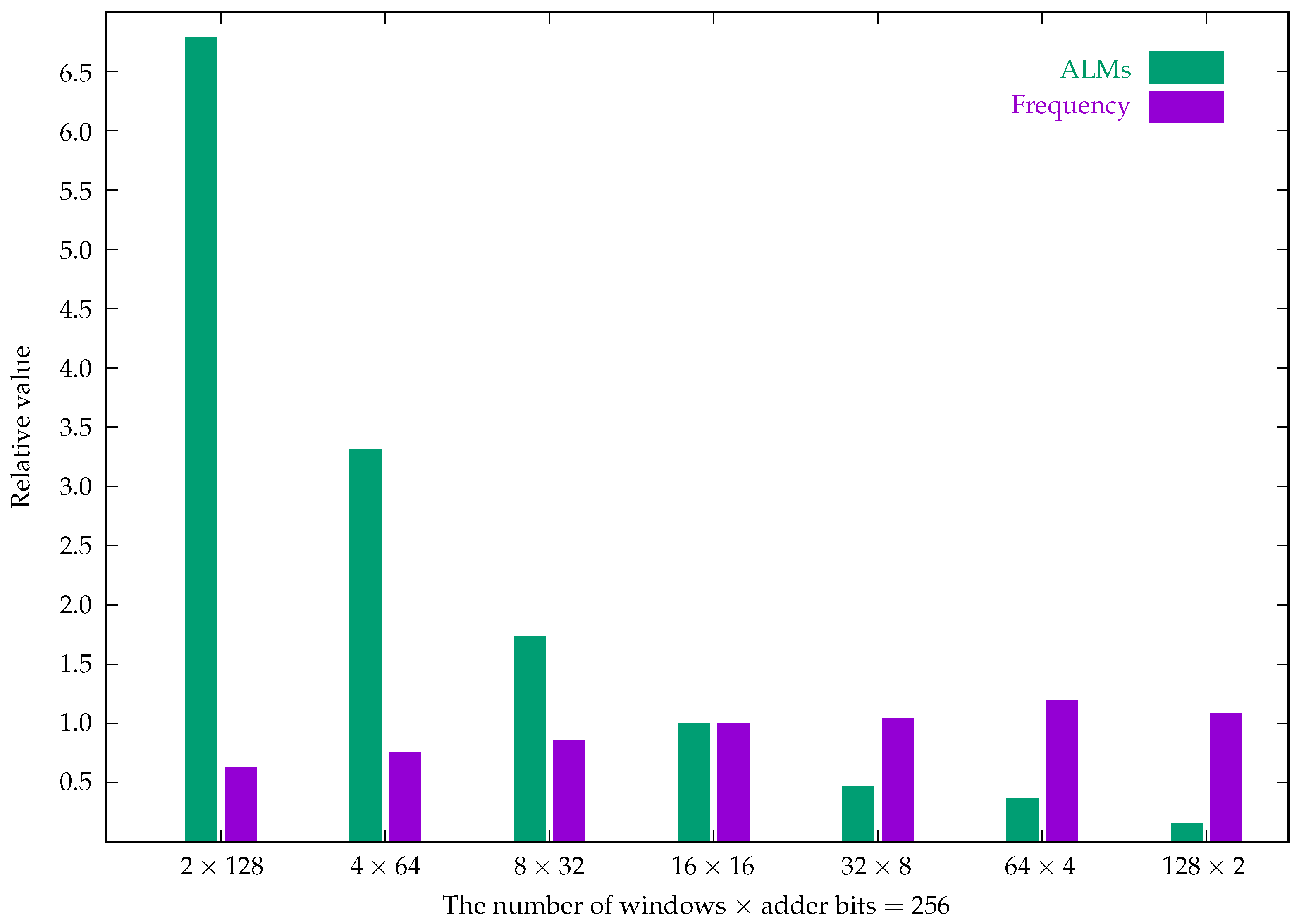
| Windows × Adder Bits | |||||||
|---|---|---|---|---|---|---|---|
| ALMs | 129 | 63 | 33 | 19 | 9 | 7 | 3 |
| Frequency (MHz) | 205.30 | 248.57 | 282.09 | 326.90 | 342.58 | 392.46 | 355.75 |
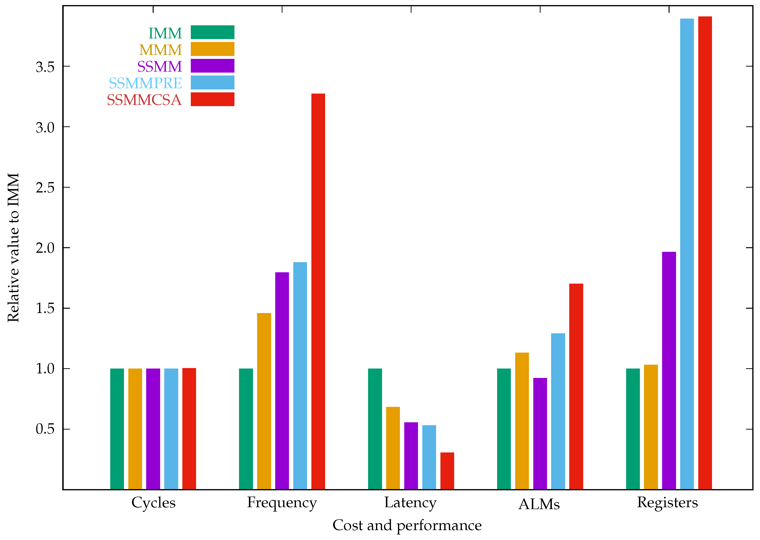
| Algorithm | Cycles | Freq. (MHz) | Latency (μs) | ALMs | Registers | Power S/D (mw) |
|---|---|---|---|---|---|---|
| IMM | 258 | 35.61 | 7.25 | 656 | 268 | 358.61/176.66 |
| MMM | 258 | 51.97 | 4.96 | 742 | 277 | 359.09/162.15 |
| SSMM | 258 | 63.97 | 4.03 | 606 | 527 | 353.73/117.67 |
| SSMMPRE | 258 | 66.92 | 3.86 | 847 | 1043 | 354.06/214.35 |
| SSMMCSA | 259 | 116.58 | 2.22 | 1117 | 1048 | 353.98/161.25 |
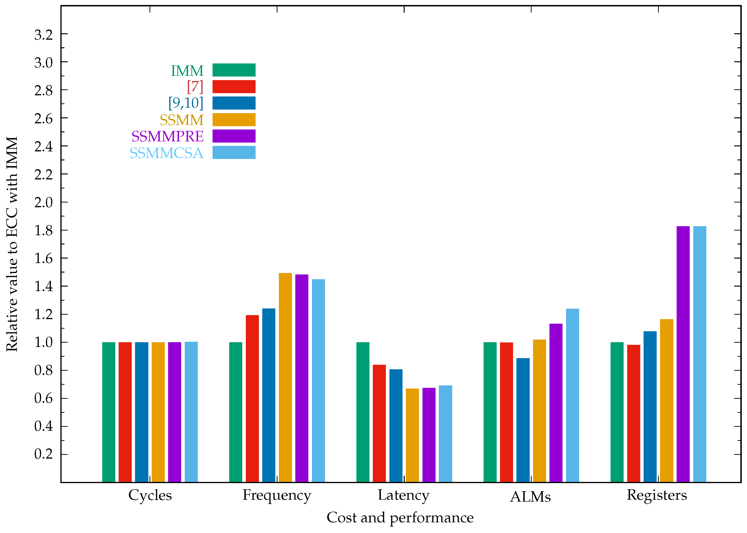
| Algorithm | Cycles | Freq. (MHz) | Latency (ms) | ALMs | Registers | Power S/D (mw) |
|---|---|---|---|---|---|---|
| ECC implementations in affine coordinates | ||||||
| IMM | 402,146 | 13.50 | 29.79 | 14,828 | 7181 | 351.63/544.03 |
| [7] | 402,146 | 16.10 | 24.98 | 14,790 | 7046 | 351.47/511.51 |
| [8] | 402,146 | 15.55 | 25.86 | 14,526 | 6593 | 351.35/484.90 |
| [9,10] | 402,146 | 16.74 | 24.02 | 13,139 | 7739 | 351.16/447.03 |
| SSMM | 402,146 | 20.16 | 19.95 | 15,096 | 8354 | 351.63/543.72 |
| SSMM-WE | 402,146 | 20.16 | 19.95 | 15,096 | 8354 | 351.63/543.72 |
| SSMM-AND | 402,146 | 16.18 | 24.85 | 15,088 | 8353 | 351.55/527.63 |
| SSMMPRE | 402,146 | 20.02 | 20.09 | 16,782 | 13,111 | 352.25/688.02 |
| SSMMCSA | 403,166 | 19.56 | 20.56 | 18,372 | 13,119 | 352.11/640.69 |
| ECC implementations in projective coordinates | ||||||
| IMM | 396,550 | 17.17 | 23.10 | 30,286 | 15,333 | 352.33/694.29 |
| [7] | 396,550 | 21.27 | 18.64 | 29,958 | 14,944 | 352.30/688.05 |
| [8] | 396,550 | 19.72 | 20.11 | 28,467 | 13,001 | 352.00/628.22 |
| [9,10] | 396,550 | 21.19 | 18.71 | 20,253 | 13,179 | 351.05/434.50 |
| SSMM | 396,550 | 29.97 | 13.23 | 29,826 | 23,811 | 352.24/676.44 |
| SSMM-AND | 396,550 | 20.30 | 19.53 | 29,771 | 23,736 | 352.18/664.67 |
| SSMMPRE | 396,550 | 29.36 | 13.51 | 37,508 | 42,198 | 353.50/926.33 |
| SSMMCSA | 398,080 | 21.81 | 18.25 | 47,083 | 48,424 | 353.46/919.52 |
| ECC implementations in Jacobian coordinates | ||||||
| IMM | 369,079 | 14.11 | 26.16 | 27,861 | 14,237 | 351.98/625.50 |
| [7] | 369,079 | 16.63 | 22.19 | 27,630 | 13,561 | 351.78/583.41 |
| [8] | 369,079 | 16.33 | 22.60 | 26,306 | 11,733 | 351.71/568.49 |
| [9,10] | 369,079 | 17.63 | 20.93 | 19,311 | 12,124 | 350.90/403.49 |
| SSMM | 369,079 | 21.23 | 17.38 | 28,993 | 21,862 | 352.74/777.09 |
| SSMM-AND | 369,079 | 16.44 | 22.45 | 28,734 | 22,296 | 352.51/730.81 |
| SSMMPRE | 369,079 | 20.75 | 17.79 | 35,840 | 39,724 | 354.46/1114.60 |
| SSMMCSA | 370,502 | 16.79 | 22.07 | 44,624 | 45,382 | 354.09/1042.09 |
Disclaimer/Publisher’s Note: The statements, opinions and data contained in all publications are solely those of the individual author(s) and contributor(s) and not of MDPI and/or the editor(s). MDPI and/or the editor(s) disclaim responsibility for any injury to people or property resulting from any ideas, methods, instructions or products referred to in the content. |
© 2023 by the author. Licensee MDPI, Basel, Switzerland. This article is an open access article distributed under the terms and conditions of the Creative Commons Attribution (CC BY) license (https://creativecommons.org/licenses/by/4.0/).
Share and Cite
Li, Y. Hardware Implementations of Elliptic Curve Cryptography Using Shift-Sub Based Modular Multiplication Algorithms. Cryptography 2023, 7, 57. https://doi.org/10.3390/cryptography7040057
Li Y. Hardware Implementations of Elliptic Curve Cryptography Using Shift-Sub Based Modular Multiplication Algorithms. Cryptography. 2023; 7(4):57. https://doi.org/10.3390/cryptography7040057
Chicago/Turabian StyleLi, Yamin. 2023. "Hardware Implementations of Elliptic Curve Cryptography Using Shift-Sub Based Modular Multiplication Algorithms" Cryptography 7, no. 4: 57. https://doi.org/10.3390/cryptography7040057
APA StyleLi, Y. (2023). Hardware Implementations of Elliptic Curve Cryptography Using Shift-Sub Based Modular Multiplication Algorithms. Cryptography, 7(4), 57. https://doi.org/10.3390/cryptography7040057