Abstract
In this paper, we present approaches to generating random numbers, along with potential applications. Rather than trying to provide extensive coverage of several techniques or algorithms that have appeared in the scientific literature, we focus on some representative approaches, presenting their workings and properties in detail. Our goal is to delineate their strengths and weaknesses, as well as their potential application domains, so that the reader can judge what would be the best approach for the application at hand, possibly a combination of the available approaches. For instance, a physical source of randomness can be used for the initial seed; then, suitable preprocessing can enhance its randomness; then, the output of preprocessing can feed different types of generators, e.g., a linear congruential generator, a cryptographically secure one and one based on the combination of one-way hash functions and shared key cryptoalgorithms in various modes of operation. Then, if desired, the outputs of the different generators can be combined, giving the final random sequence. Moreover, we present a set of practical randomness tests that can be applied to the outputs of random number generators in order to assess their randomness characteristics. In order to demonstrate the importance of unpredictable random sequences, we present an application of cryptographically secure generators in domains where unpredictability is one of the major requirements, i.e., eLotteries and cryptographic key generation.
1. Introduction
Is there a method to generate a sequence of truly random numbers? Can we really prove that a sequence of numbers is really random? For instance, which of the following two 26-bit sequences is “random”?
- Sequence : 10101010101010101010101010.
- Sequence : 01101011100110111001011010.
By which criteria, however? Without a precise definition of “randomness”, no mathematical proof of randomness can be attained. “Intuition” is, often, not sufficient, and it may also be misleading in trying to precisely define “randomness”. Some “randomness” viewpoints that have been proposed in the literature include the following:
- A process generated by some physical or natural process, e.g., radiation, resistor or semiconductor noise (the practitioner’s view).
- A process that cannot be described in a “few words” or succinctly (the instance or descriptional complexity view)—the smaller the description of a sequence of bits can be made, the less random it is (try to apply this to the two sequences above).
- A process that cannot be guessed in a “reasonable” amount of time (the computational complexity view).
- A process that is fundamentally impossible to guess (the “philosophical” view).
- A process possessing certain statistical characteristics of the ideally uniform process (the statistician’s view).
To see that intuition may not be sufficient, observe that each of the two sequences, and , has exactly the same probability of appearing as the output of a perfect randomness source that outputs 0 or 1 with equal probability, i.e., . This probability is equal to . Yet, sequence appears “more random” than sequence , at least in the descriptional complexity view.
John Von Neumann’s verdict is the following: “Any one who considers arithmetical methods of producing random digits is, of course, in a state of sin. For, as has been pointed out several times, there is no such thing as a random number—there are only methods to produce random numbers, and a strict arithmetic procedure of course is not such a method”. True randomness is a tough task. Ideally, a number generated at a certain time must not be correlated with previously generated numbers in any way. This guarantees that it is computationally infeasible for an attacker to determine the next number that a random number generator will produce.
Whether there really exists randomness in the universe (if, indeed, “God plays dice”, a thesis that Albert Einstein famously denounced) is a fascinating but elusive scientific and philosophical question that has yet to be definitely answered. Fortunately, the mathematical theory of computational complexity and cryptography bypasses this difficulty and offers an “Apostolic Pardon” to the “sin” described by Von Neumann. In this context, a sequence is considered “random” if its efficient predictability would imply solving, efficiently, a hard computational problem, most often in number theory. Such problems are the factoring and the discrete logarithm in certain finite fields. In this way, the elusive concept of “randomness” acquires a “behavioural” substance, according to which a sequence is judged to be random based on its “behavior” as seen by an outside observer. In other words, a sequence is considered random if it is computationally difficult for an observer with reasonable computational resources at their disposal to predict it. The classical concept of randomness is, in contrast, rather “ontological” and focuses the observation on the sequence itself (the “being”, that is) to characterize it as random or non-random. The “behavioristic” approach, however, leads to interesting and very useful results for use in practical applications such as electronic lotteries, where unpredictability is a major requirement. An excellent source of papers focused on philosophical questions about randomness, as well as the interplay between randomness and computation theory, is the collective volume [1].
On the practical side, with the rapid development of algorithms for generating random numbers used in software testing, simulations, and mathematical modeling, multiple problems have been observed regarding the randomness properties of these algorithms. Thus, another interesting problem in the field of random number generation is how to characterize “randomness”, i.e., how to decide if a given, sufficiently long sequence of numbers is indeed random according to some well-defined and precise criteria. Unfortunately, all available mathematical characterizations of randomness, such as descriptive complexity, are formally undecidable. However, a number of statistical tests that can be used to, at least, provide a scale of measurement that can rank random number generators according to the statistical characteristics of the sequences they produce have been proposed. Such tests include the Diehard statistical test suite as well as other similar tests [2,3,4]. In particular, George Marsaglia proposed and implemented the Diehard randomness test suite, which includes several statistical tests that capture different aspects of randomness in sequences of numbers produced by generators (see Section 4.2 and also [5] for a complete presentation of the tests and their implementation). These tests are focused, mainly, on rejecting random number generators that exhibit undesirable, for a random sequence of numbers, properties, such as short period, patterns within the binary digits, and non-uniform distribution of the numbers. The Diehard tests are considered among the most reliable randomness tests, since the algorithms that pass these tests also perform well in practice with respect to the randomness properties of the produced numbers.
In this paper, our focus is not on wide coverage of several approaches in random generation and randomness tests but rather to try to explain basic principles and the rationale behind the tests we will describe. The paper is organized as follows: In Section 2, the importance of entropy as a measure of the strength of a source of randomness is presented. Moreover, the structure of an entropy source model as recommended by the NIST and its two types, physical and non-physical, are given. The operation of some recent true random number generators (TRNGs for short) are presented. Since existing TRNG designs are difficult to deploy in real computing systems to greatly accelerate or support target applications because the entropy sources they are based on need special treatment to be part of the target application, algorithms that generate pseudorandom numbers (pseudorandom number generators, or PRNGs for short) were developed. In Section 3, we cover the simple linear congruential generators, which are nevertheless predictable, given the sufficiently long sequence they produce as output, and the cryptographically secure generators, with unpredictability guarantees based on the computational difficulty of number theoretical problems. Coverage of several statistical tests that can be used to, at least, evaluate the implementations of the generators in order to identify weak or faulty implementations whose quality is reflected in the results of the tests is provided in Section 4. Finally, in Section 5, we present an application of cryptographically secure generators in domains where unpredictability is one of the major requirements, i.e., cryptographic key generation and eLotteries. We show how different components, such as true random number generators, cryptographically secure generators, seed quality enhancement techniques, post-betting prevention and ciphers, can be combined in order to produce long sequences of unpredictable numbers.
2. Sources of Randomness
The central mathematical concept involved in random number generation processes is entropy. Intuitively speaking, entropy reflects the uncertainty associated with predicting the value of the outcome of an experiment prior to observation (in our case, the experiment is the generation process). There are many possible measures of entropy. The most common concepts are Shannon entropy and min-entropy, recommended by the National Institute of Standards and Technology (NIST) in [4] as a very conservative measure. In [6], the reader can find more about entropy measures. Let X be an independent discrete random variable that takes values for with probability for . The min-entropy of X is defined by
It is obvious that is maximized when X has a uniform probability distribution, i.e., , and equals . This means that the uncertainty of predicting the next value of X is maximum when its probability distribution is uniform. A source of randomness (a source of random values) is modeled as an independent discrete variable and is considered an entropy source. The NIST model for an entropy source comprises a noise source; a digitization unit if the noise source is analog; an optional postprocessing unit, which increases the entropy of the generated output bits; and a health tests unit, which ensures that the entire entropy source operates as expected. There are two kinds of noise sources: non-physical and physical (see [2,7]). Depending on the noise source, there are two kinds of entropy sources: non-physical entropy sources and physical entropy sources. A non-physical noise source exploits system data (system time, RAM data, etc.) or user interactions, like mouse movement and clicks, keyboard strokes, etc. [8].
A physical entropy source exploits a physical noise source that exhibits variations in some of its properties or characteristics. A small change in the source at a certain time progressively impacts future conditions in the system over time. Such a noise source can be tapped in order to produce an infinite sequence of bits, e.g., by converting the analogue values of the variations into digital form. For this reason, it is necessary that the deployed physical noise sources have sufficiently varying random fluctuations in the properties used to draw randomness. Physical noise sources with good properties are Geiger counters, zener diodes, ring oscillators [9,10] and digital-to-analog converters (DACs) [11]. These sources appear to produce bits that do not follow some easily predictable pattern. However, as time progresses, they sometimes appear to produce long streaks of 0 s alternating with long streaks of 1 s, which is undesirable. In [12], a true random number generator (TRNG) that is composed of an entropy source based on a semiconductor-vacancy junction and a DAC-based square transformer in the voltage domain is presented. Another example of TRNG design, named resilient high-speed (RHS)-TRNG, appears in [13]. It is a TRNG circuit based on a spin-transfer torque magnetic tunnel junction (STT-MTJ) that, by circuit/system codesign, was integrated into an RISC-V processor as an acceleration component and driven by customized random number generation instructions.
Nowadays, physical unclonable functions (PUFs), which consist of inherently unclonable physical systems, are used as sources of randomness. Their unclonability arises from their many random constituent components that cannot be controlled. When a stimulus C is applied to a PUF device, it reacts with a response R. This pair is called a challenge–response pair (CRP). Thus, a PUF can be considered a function that maps challenges to responses. A response to a challenge cannot be exploited to discover another response to a different challenge , with [14]. Moreover, it is impossible to recover response corresponding to a challenge without having the right PUF that can produce it. If an attacker tries to analyze the PUF in order to learn its structure, the response behavior of the PUF is changed substantially. A PUF is considered strong if along with the above properties, there is a large number of challenge response pairs , , available for the PUF [14]. In [15], a hardware random number generator (HRNG) that is based on these large numbers of pairs is presented. A classical RNG sends challenges to a PUF, which reacts with the corresponding responses, and these responses are used for the bit construction of the random number.
However, due to the existence of noise while a PUF operates, when it is challenged with , a response , which is a noisy version of , is obtained. For this reason, each time, a PUF produces helper data, which can be used by error correction code to recover . On the other hand, random number generators need a non-deterministic source of entropy. Subsequently, the noise from the PUF response can be used for that purpose. So, it makes sense to use the noise from a PUF as a source of entropy to extract a true random seed. In [16], a systematic review of various entropy sources that are based on silicon primitives, TRNGs and PUFs, is presented. Chaos-based, jitter-based, noise-based and metastability-based entropy sources are four types of sources that a silicon TRNG can use to harvest randomness. Moreover, the models of silicon-based PUF devices that harvest randomness from the physical properties of its integrated circuit are analyzed.
Now, the question that arises is whether we can produce a random (or at least a “seemingly” random) sequence of numbers using physical entropy sources that are not sufficiently random for the purpose at hand (e.g., they do not follow the uniform distribution). John von Neumann was one of the first to attempt to address this question. According to the model he considered, suppose that we have a randomness source that produces a sequence of bits with the property that for all i, , for some . Then, from this source, we can generate a random sequence with the following algorithm: For each pair 01 of bits produced by the source we consider, 0 is returned, while 1 is returned for each pair 10. For 00 or 11, no bit is returned. The von Neumann model is limited, because the probability value () is assumed to be fixed, while it also has the disadvantage that from a source that may produce a very large number of bits, several of them are discarded.
Santha and Vazirani’s model is less restrictive. A source is called an SV source (Santha–Vasirani source) if for some real number , it holds that for all i. A random sequence is called minimally random if it has been produced by an SV source. When , then the sequence is considered random. Santha and Vazirani proved that if , then a truly random sequence cannot be produced from a minimally random sequence. That is, for every algorithm that produces a sequence X with a minimally random sequence as input, there is a corresponding algorithm for which or .
The next question that thus arises is whether the combination of several SV sources can produce a more random sequence. Before answering this question, we define the concept of a semi-random source. A source is said to be semi-random if for every and every function , the following holds for all large integers n and for all n-bit sequences :
Semi-random sources, as defined by (1), are almost indistinguishable from truly random sources. Therefore, if we can produce a semi-random sequence from a minimally random source (or several such sources together, e.g., by XORing their outputs), we have constructed a sufficiently strong randomness source.
Given m independent, minimally random sources as input, the following algorithm produces a semi-random sequence. We assume that is given and , where n is a large integer.
Algorithm 1 can be used in practical applications using the outputs of several physical entropy sources. It is convenient and one of the most efficient algorithms for converting, possibly, minimally random physical random sequences into semi-random sequences.
| Algorithm 1 Combining the outputs of several physical entropy sources |
| for do |
| Generate minimally random sequences from source |
| end for |
| return |
3. Pseudorandom Number Generation
As we discussed in Section 2, using physical sources of randomness may not be convenient in several application domains. Existing TRNG designs are difficult to deploy in real computing systems to greatly accelerate or support target applications because the entropy sources they are based on need special treatment to be part of the target application.
Fortunately, for almost all cryptographic applications, pseudorandom numbers can be used, i.e., numbers that appear to be truly random to someone attempting to interfere, maliciously, with the application. Algorithms that generate pseudorandom numbers, i.e., pseudorandom sequences of bits, are called pseudorandom number generators, or PRNGs for short.
The generation of pseudorandom numbers involves the production of long sequences of bits starting from a small, preferably truly random initial value called seed. Among the desirable properties that are expected from a PRNG is the generation of uniformly distributed bits, i.e., bits that could have been produced by successive flips of an unbiased coin. Naturally, pseudorandom sequences can never be completely random in the sense of predictability. In particular, given any pseudorandom sequence that has been produced by an algorithm using an initial seed value, an exhaustive search among all possible seed values could identify the seed from which the observed numbers were produced. However, the required time may be prohibitively long. For some classes of PRNGs, however, such as the linear congruential generators discussed in Section 3.1, there are more efficient ways to uncover future values given an initial segment of the pseudorandom sequence.
This fact leads to the question of how to design PRNGs that are unpredictable in reasonable (i.e., polynomial) time. As an answer to this question, the concept of cryptographically secure PRNGs was first proposed by Blum and Micali [17] and Yao [18]. A PRNG is called cryptographically secure if it passes all polynomial time statistical tests or, in other words, if the distribution of bit sequences it produces cannot be separated from truly random sequences by any polynomial time algorithm. On the other hand, a PRNG is called polynomially predictable if there exists a polynomial time algorithm that, given a sufficiently long sequence of bits produced by the generator, can predict its next outputs. For example, the linear congruential (LCGs—see Section 3.1) and generators are polynomially predictable. In contrast, BBS and RSA (see Section 3.2.1 for a discussion on BBS) are polynomially unpredictable. For this reason, such generators are the generators of choice in applications where unpredictability is a major requirement, such as in the implementation of electronic lotteries (see [19,20] and Section 5), key generation and network security protocols.
A key definition in the area of cryptographically secure PRNGs is the following (see [21]).
Definition 1
(Pseudorandom function). A family of functions , indexed by a key , is said to be pseudorandom if it satisfies the following two properties:
- Easy to evaluate: The value of is efficiently computable given s and x.
- Pseudorandom: Function cannot be efficiently distinguished from a uniformly random function , given access to pairs , where the can be adaptively chosen by the distinguisher.
More specifically, we say that a pseudorandom generator is polynomially unpredictable if and only if, for every finite initial part of the sequence produced by that generator and for every bit erased from that part, a probabilistic Turing machine cannot guess this bit in polynomial time. In other words, there is no better way to determine the value of this bit than flipping an unbiased coin.
In cryptographically secure generators, the difficulty of predicting their outputs is based on the difficulty of solving a mathematical problem, most often from algorithmic number theory. For these problems, there is no algorithm that solves them in probabilistic polynomial time. Integer factorization (factoring problem), the discrete logarithm problem in finite fields and elliptic curves (discrete logarithm problem), and the quadratic residuosity assumption are among the most prominent of these problems. Thus, we may say that a generator is cryptographically secure if the solution to a difficult mathematical problem, like the ones listed above, is reduced to predicting the next bit of the sequence given the first polynomially numerous bits of the sequence. Formally, a -PRNG is a polynomial (in k) time function . Input is the seed, and are positive integers, with . Output is a sequence of bits and is called pseudorandom bit string. Function f is said to be a cryptographically strong PRNG if it has the following properties:
- Bits are easy to calculate (for example, in polynomial time in some suitable definition of the size parameter, e.g., the size of a modulus).
- Bits are unpredictable in the sense that it is computationally intractable to predict in sequence with probability better than ; i.e., for any computationally feasible next-bit predictor algorithm ,for .
3.1. The Linear Congruential Generator
The well-known linear congruential generator (LCG) produces a recursively defined sequence of numbers calculated with the following equation:
In this equation, is the initial state or seed; a is the multiplier; c is the increment; and m is the modulus. The various choices for generator parameters a, c and m define periodq of the generator. This is the minimal value of q such that (see the excellent exposition in [22]).
The range of most common LCGs is limited to values of ; thus, they do not have good statistical properties. Therefore, their use in simulations (e.g., Monte Carlo) is limited. In applications where m can be arranged to be of the size of several hundred or even thousand of bits, this issue can be addressed. However, although current microprocessor technology has progressed significantly and allows for the implementation, in hardware, of increased precision integer arithmetic, for such values of m, it is necessary to implement, in software libraries, arbitrary precision integer arithmetic, which may be too expensive for practical purposes.
It is easy to see that the maximum period for an LCG is equal to m. To obtain this upper bound, however, the following conditions should be met (see, e.g., [22]):
- Parameter c should be relatively prime to m.
- If m is a multiple of 4, then should also be a multiple of 4.
- For all prime divisors p of m, the value of should be a multiple of p.
The reader may consult [22] for more mathematical properties and details of LCGs in the form shown in Equation (3). Popular programming languages most often deploy LCGs for the generation of pseudorandom number sequences, since strong security properties (mainly unpredictability) are not of concern in customary programming projects where the focus is on the randomness (i.e., statistical) properties of the sequences. See, however, Section 5 of this survey paper for the presentation of an application domain, electronic lotteries, where unpredictability properties are essential.
There exist several variations of the LCGs as given in (3). It is possible, for instance, to set as the increment value. The resulting generator is termed multiplicative or mixed generator (in short MCG) and has the form
As a consequence of setting , less operations are needed; thus, the generation of numbers using (4) is faster (albeit slightly) than the generation of numbers using (3) when . However, it is not possible to obtain the maximum period (i.e., m), since, for instance, the value 0 cannot appear unless the sequence itself is composed of all 0 s.
In addition, if and is relatively prime to m for all values of n, then the length of the period of the sequence cannot exceed , which is the cardinality of the set of integers between 0 and m that have the property of being relatively prime to m (see, e.g., [22]). Now, if , where p is a prime number and , Equation (4) reduces to
If a is relatively prime to p, then the period of the MCG is the least , such that . If is the GCD of and , then this condition reduces to .
If a is relatively prime to m, then the smallest integer for which is termed order of , and all values a that have maximum possible order modulo m form the set of primitive elements modulo m. Thus, the maximum possible period for MCGs is equal to the order of a primitive element (i.e., maximum possible order) modulo m. This is equal to (see, e.g., [22])) whenever the following apply:
- m is prime;
- a is a primitive element modulo m;
- is relatively prime to m.
With respect to predictability, LCGs do not possess good properties. In [23,24,25], efficient algorithms are presented for predicting the next value given past values of the LCG even if some bits of these values are missing (i.e., they have not been given publicly).
3.2. Cryptographically Secure Generators
Since cryptographically secure PRNGs are accompanied by strong security (unpredictability) evidence, we present some of the most powerful cryptographically secure PRNGs, and we discuss design directions for the construction of such PRNGs.
3.2.1. The BBS Generator
The BBS generator, proposed by L. Blum, M. Blum and M. Shub in [26], is one of the most often deployed cryptographically strong PRNGs. Its security (unpredictability) is founded on the difficulty of the quadratic residue problem.
For every integer N, is its length in bits, and , its length in base . If , is the set of finite sequences with elements from , and , the set of sequences with an infinite number of elements from . Also, we define , i.e., the set of finite sequences of length k. For all sequences , we denote by the initial part of sequence x of length k (i.e., its first k elements), and we denote by the k-th element of x (its first element is ).
We denote by the smallest non-negative integer remainder from dividing x by integer N. A quadratic residue is any number x for which there exists an integer u such that . Recall that integers and , i.e., the set of integers that are smaller than N and relatively prime with N. Set has order, i.e., number of elements, equal to . The set of quadratic residues modulo N is denoted by . This is a subset of and has order . Additionally, we denote by the subset of consisting of its elements that have a Jacobi symbol equal to 1 and by the subset of its elements that have Jacobi symbol . All quadratic residues belong in subset .
Each quadratic remainder has four different roots in , which are and . If, however, we assume that , then every quadratic residue has exactly one square root, which is also a quadratic residue. In other words, the function is a and onto mapping (i.e., bijection) from to itself.
Finally, we state the definition of Carmichael’s function, which will also be needed for the concept of special primes. Carmichael’s -function [27] is closely related to Euler’s totient function. However, while Euler’s totient function provides the order of unit group , Carmichael’s function provides its exponent. In other words, is the smallest positive integer for which it holds that for any a that is coprime to n. Carmichael’s function is not multiplicative but has a related property, which can be called lcm-multiplicative, as follows:
Some special values include , for an odd prime power, , , as well as for . Based on these special values and Equation (5), can be computed for any positive integer n.
A prime number P is called special if and , where are primes greater than 2. A composite number is special if and only if P, Q are two distinct special primes and .
Set of the generator parameters consists of all positive integers , where P, Q are distinct prime numbers of equal length (i.e., ) and . For any integer N, set is the set consisting of the quadratic residues . The domain of the generator seeds is . The seeds should be selected from X according to the uniform distribution for increased generator security.
Given as input a pair , the BBS pseudorandom number generator outputs a pseudorandom sequence of bits , where and . is the least significant bit of integer x. The construction of the pseudorandom sequence obviously takes place in polynomial time. As it is shown in [26], the period () of the pseudorandom sequence divides or is equal to (under some condition) . Given and , we can efficiently calculate for . To calculate for , we use the equality . As we will see below, if and N are known, but not the values of P and Q, we can construct the pseudorandom sequence forward (i.e., for ) but not backwards (for ). thus, it appears that the prediction of the sequence is as hard as factoring a large integer . Alexi et al. [28] proved that the BBS generator remains cryptographically secure even if it outputs up to low-order bits instead of only one. With this result, the generator’s efficiency is greatly improved. Practically, a BBS generator can be realized as follows:
- Find primes p and q such that mod 4.
- Set .
- Start with = seed (a truly random value), .
- Set mod N.
- Output the least significant bit of .
- Set , go to step 3.
Now, regarding the security of this generator, as mentioned above in the introduction, all cryptographically secure generators base their security on the difficulty of solving number theory problems. This problem, in the case of the BBS generator, is the quadratic residuosity problem. The problem is defined as follows: Given N and , decide whether x is a quadratic residue . Recall that exactly half the elements of are quadratic residues.
The quadratic residuosity assumption states that any efficient algorithm for solving the quadratic residuosity problem would give wrong results for at least a percentage of the inputs to the algorithm. More formally, the assumption is as follows: Let be a polynomial and be a polynomial algorithm that, when given as input N and x, with , returns 0 if x is not a quadratic residue and 1 otherwise. Also, let be a constant and t be a positive integer. Then, for n very large and for a fraction d of numbers N, with , the probability that process gives the wrong answer for integer x (given that x is chosen according to the uniform distribution from ) exceeds , that is, . The quantity can be replaced with .
The details of the discussion that follows can be found in [26]. We also recall that in what follows, , with P, Q prime numbers and , and that the function is a mapping from QRN to QRN.
According to the definition of the BBS generator, knowledge of N is sufficient for the efficient generation of the sequence starting from a seed value . However, knowing only N and not its two factors P and Q does not suffice for the generation of the sequence in reverse direction, i.e., the sequence starting from . For this purpose, factors P and Q are needed. This necessity follows from the following argument: Suppose that we can efficiently calculate without knowing the factors of N. Then, in order to factor N, we choose an , and we set and calculate . We then compute or Q. Therefore, the ability to compute for at least a percentage of the values of x would allow us to factor N efficiently with a high probability of success.
On the other hand, if we could factor N, we could generate the pseudorandom sequence backwards. This fact follows from the following theorem: There exists an efficient deterministic algorithm A that, when given as inputs N, factors P and Q, and any quadratic residue , computes the unique quadratic residue for which . In other words, .
Moreover, the factors of N are necessary to have an -advantage in finding the parity bit of in polynomial time, given . A probabilistic process P that returns 0 or 1 is said to have an -advantage, with , in guessing the parity bit of if and only if . Similarly, we can define a probabilistic procedure that would have an -advantage in deciding whether some is a quadratic residue (which is the quadratic residuosity problem). More simply, we would say (according to a lemma of [26]) that an -advantage in finding the parity bit of can be converted into an -advantage for the quadratic residuosity problem.
In [26], a theorem that proves the unpredictability of the BBS generator is given. By this theorem, for any constant and any positive integer t, any probabilistic polynomial process P has at most a advantage in predicting the sequences generated by BBS backwards (for sufficiently large and for all but a fraction of N). In short, if the BBS generator were predictable, the quadratic residuosity assumption described previously would not hold. For this reason, the generator can be safely assumed to also pass every probabilistic, polynomial, statistical test on its long-term output.
Having shown that the output of the generator cannot be efficiently predicted, its period remains to be calculated. The fact that the sequence cannot be predicted shows that the period of should be very large. According to a theorem proved in [26], period divides . However, it would be best for the period to be as long as possible, i.e., equal to . The equality can indeed hold under two conditions. The first is that integer N is special as defined earlier, and the second is to choose a seed so that its order is equal to .
Finally, we define the linear complexity of a sequence of pseudorandom numbers as the smallest number L for which the linear relationship
holds for
The linear complexity of any pseudorandom sequence does not exceed the period of the sequence. Obviously, the higher the linear complexity of a sequence is, the more cryptographically secure it is with respect to the prediction of its output. As demonstrated in [29], the BBS generator does not exhibit any particular form of linear structure, a property that excludes the possibility of applying attacks such as the Lattice Reduction attack on its outputs.
3.2.2. The RSA/Rabin Generator
The second cryptographically secure generator is the RSA/Rabin generator. It is based on the RSA function, and it works as follows:
- Find primes p and q as well as a small prime e such that .
- Set .
- Start with = seed (a truly random value), .
- Set mod N.
- Output the least significant bit of .
- Set and repeat from Step 3.
The RSA/Rabin generator is cryptographically secure under the RSA function assumption. According to this assumption, given N, e and y, where , the problem of determining x is computationally intractable. More details about this generator can be found in [28].
3.2.3. Generators Based on Block Ciphers
The other two generators that are deployed in the lottery are based on the encryption algorithms DES (Data Encryption Standard) and AES (Advanced Encryption Standard). The implementations provided by version 2.5.3 of the mcrypt library (available at [30]) were used with key sizes of 64 bits for DES and 192 bits for AES.
DES and AES are used in their CFB (cipher-text feed-back) mode, and they are operated as follows: An initial random seed is constructed from the combined output of the true random generators; then, DES and AES are invoked, using the seed as the Initial Vector (IV), as many times as the values we need to generate. In particular, every time the encryption function is called, a byte with all zeros is encrypted (always in CFB mode), and the encryption result is the output of the corresponding generator.
The cryptographic strength of these two generators is based on the security of the corresponding encryption algorithms and not on a presumed computationally hard mathematical problem, like RSA and BBS. However, both generators have passed, separately, all the Diehard tests; thus, their output is considered secure.
Bruce Schneier et al., in [31], present the design and analysis of the Yarrow cryptographically secure PRNG. Yarrow relies on a one-way hash function with an m-bit digest and a block cipher with a k-bit key and an n-bit block size. The designer should select a one-way hash function that is collision-intractable (e.g., one from the SHA-2 family of hash functions) and a block cipher (e.g., AES) that is highly resistant to known-plaintext and chosen-plaintext attacks.
The major components of Yarrow are an entropy accumulator, which collects samples from entropy sources in two pools; a reseeding mechanism, which periodically reseeds the key with new entropy from the pools; and a block-cipher-based generation mechanism, which generates random numbers (Figure 1). The basic idea behind the generation mechanism is that if an attacker does not know the block-cipher key, they cannot distinguish the generated outputs from a truly random sequence of bits.
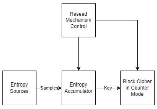
Figure 1.
Yarrow PRNG structure.
The entropy accumulator determines the next unguessable internal state of the PRNG. Each source of entropy sends samples to the entropy accumulator, and their hashed values are stored to either a fast pool or a slow pool. The fast pool is used for frequent key reseeding, while the slow one, for rare reseeding. It is obvious that the collected entropy is no more than the size of the hash digest, i.e., m-bit entropy. Initially, the entropy accumulator collects samples until the collected estimated entropy is high enough for reseeding the block cipher with a new key. Recommendations for entropy estimation can be found in [4].
3.2.4. Algorithms M and B
Given two sequences of pseudorandom numbers X and Y, algorithm M produces a sequence significantly “more random”. Essentially, the numbers in are the same as those that make up X, except that they are in different positions (i.e., they form a permutation of the original sequence, X) in the new sequence. These positions are dictated by sequence Y.
More specifically, an array N with k elements is formed, where k is an integer depending on the application, often close to 100. The elements in array N are the first k elements of sequence X. The steps of algorithm M (applied iteratively) appear in Algorithm 2.
| Algorithm 2 Description of the algorithm M |
|
It turns out that in most cases, the period of the sequence produced by algorithm M is the least common multiple of the periods of sequences X and Y.
However, there is a more effective way to transpose the elements of a sequence X. The corresponding algorithm is called Algorithm B. It is similar to M, but it achieves better results in practice. At the same time, it has the advantage that only one sequence of pseudorandom numbers is needed, and not two as in the case of M.
Initially (as in M), the first k elements of sequence X are placed in array N. Then, variable y takes the value , and the following steps are applied iteratively:
- , where m is the modulus of sequence X.
- is the next new element of sequence .
- We set , and is set to the next element of sequence X.
Although algorithm M can produce satisfactory pseudorandom number sequences, given as input even non-random sequences (e.g., the Fibonacci numbers sequence, for example), it is still likely to produce a less random sequence than the original sequences if they are strongly correlated. Such issues do not arise with algorithm B. Algorithm B does not, in any way, reduce the “randomness” of the given sequence of pseudorandom numbers. On the contrary, it increases it with a small computational cost. For these reasons, it is recommended to use algorithm B with any PRNG. Both algorithms are described in detail in Knuth’s book [22].
A notable disadvantage of algorithms M and B is that they only modify the order of the numbers in a sequence and not the numbers of the sequences themselves. Although, for most applications, the ordering of the numbers is important, if the initial generators we choose do not pass some basic statistical tests, permuting their elements with the M and B algorithms does not render them stronger. For this reason, in applications that require pseudorandom number sequences with strong randomness properties with theoretical guarantees that imply unpredictability, it is better to deploy cryptographically secure PRNGs, such as BBS and RSA, optionally using algorithms M and B.
4. Randomness Tests
In general, the quality of a pseudorandom number generator is based on a specific theoretical framework that provides the assumptions and requirements that lead to a series of theoretical results demonstrating various quality aspects, such as long period and unpredictability.
Although mathematical evidence should be sufficient, an implementation of a generator should be able to demonstrate, in practice, specific quality aspects. For this reason, the design and implementation of pseudorandom number generation algorithms should also be accompanied by the results of statistical or randomness tests that attest to the quality properties of the algorithms or, at least, their specific implementations.
Before we continue, in the probability calculations for some of the tests that follow, Stirling numbers of the second kind are needed. A Stirling number of the second kind denotes the number of ways a set of n indistinguishable elements can be partitioned into k non-empty indistinguishable subsets, where each subset should contain at least one element. The notation for Stirling numbers of the second kind is , and they are defined, algebraically, as follows:
As we discussed in the Section 1, some quality properties of random number generators are hard to define and evaluate using practical, i.e., finite and computable, approaches. For instance, unpredictability and randomness themselves are elusive concepts with various theoretical characterizations, most of which do not lead to practical, computable tests. After all, algorithms and computers are deterministic entities whose time evolution follows a well-defined sequence of steps in order to produce results.
On the other hand, the science of statistics can provide approaches and tools for evaluating, empirically, some measurable properties related to the “randomness” of a number sequence. The generated sequences are evaluated with respect to their randomness behavior according to certain statistical tests’ assumptions and rules.
These tests are designed so that the expected values of a test’s statistical indicators are known to hold for a uniform distribution. Then, the generated sequence is subjected to the test, and the results are compared with the results that a perfectly uniformly random generated sequence would give. Although a variety of tests can be applied to a sequence produced by a PRNG, research in this field has provided guidelines as to which tests are most appropriate and efficient. In general, PRNGs that pass these tests are considered acceptable for generating pseudorandom numbers. For instance, a number of tests are described in [22], several of which are implemented in the Diehard randomness test suite (see [5]), and some of them are recommended by the NIST in [3]. In what follows, we will describe a number of these tests and discuss the randomness properties they evaluate.
4.1. Practical Statistical Tests
In this section, we will present a number of statistical tests described in Knuth’s book [22]. Most of the tests, however, suit mainly truly random number sequences, while some of the test parameters are not provided numerically. Thus, we follow the modifications of these tests as described in [32], which are appropriate for integer number sequences, while specific parameter values are provided for the tests.
In particular, the basic theory of tests for real number sequences is provided in [22]. The proposed applicability criteria are also suitable for integer sequences in some tests. However, integer sequences cannot be tested, since the same assumptions as for real number sequences may not be applicable to integers. For instance, the Permutation Test gives test probabilities based on the premise that no two consecutive terms of the tested sequence can be equal. However, for integer sequences, equality of consecutive terms may occur with a non-negligible probability. Thus, in [32], new combinatorial calculations were developed in order to adapt Knuth’s test suite to integer and binary sequences. Additionally, some of the required parameters for the tests, such as the sequence length, the alphabet size, the block size, and other similar parameters, are also provided in [32]. Taking into account the aforementioned issues, the authors of [32] provide the test details and the required probability calculations for testing binary and integer sequences, which are of interest for our purposes.
Each of the tests is applied, in general, to a sequence of real numbers, which, assumedly, have been chosen independently from the uniform distribution in the interval . However, some of the tests are designed for sequences of integers rather than sequences of real numbers. Thus, we form the auxiliary integer sequence , where . Parameter d should be sufficiently large so that the tests’ results are meaningful for our PRNGs (e.g., the that fall in the PRNG’s range) but not so large as to render the test infeasible in practice. Accordingly, this sequence has been assumedly produced through independent choices from the uniform distribution over the integers .
Below, we discuss some of the tests in Knuth’s book [22]. One may also consult their modified form provided in [32]. We first discuss two fundamental tests that are used in combination with other empirical tests that we describe afterwards.
4.1.1. The “Chi-Square” Test
In probability theory and statistics, the “chi-squared” distribution, also called “chi-square” with k degrees of freedom and denoted by , is defined as the distribution of the sum of the squares of k standard normal random variables. The “chi-square” distribution of k degrees of freedom is also denoted by or . The “chi-squared” distribution is one of the most frequently used probability distributions in statistics, e.g., in hypothesis testing and in the construction of confidence intervals.
In our case, the “chi-square” distribution is used to evaluate the “goodness-of-fit” of the monitored frequencies of a sequence of observations to the expected frequencies of the distribution under test (this is the hypothesis). The test statistic (stochastic distribution) is of the form , where and are the observed and expected frequencies of occurrence of the observations, respectively. This chi-square test is one of the most widespread statistical tests of a sequence of data derived from observations of a process, in general. In our case, this process is the generation of pseudorandom numbers, and our data are the generated numbers.
We assume the following:
- Each observation can belong to one of k categories.
- We have obtained n independent observations.
According to this test, we perform n independent observations from a pseudorandom number generator (n should be large enough). In our case, the observations are pseudorandom numbers. Then, we count how many times each number appears. Let us assume that the number s appears times. Also, let be the probability of appearance of s. We calculate the following statistical indicator (we assume that the numbers generated by the pseudorandom number generator are within the range ):
Next, we compare V to the entries of the distribution tables of with the degree of freedom k equal to . If V is less than the table entry corresponding to 99% or greater than the entry corresponding to 1%, then we do not have sufficient randomness. If it is between the entries of 99% and 95%, then insufficient randomness may exist. A value below 95% is a good indication that the numbers under test are close to random.
Knuth suggests applying the test to a sufficiently large sequence of numbers, i.e., for large values of n. Also, for test reliability purposes, he suggests, as a rule of thumb, that n should be sufficiently large to render the expected values of greater than 5. However, a large value of n presents some undesirable properties, such as locally non-random behavior through, for instance, an entrance into a cycle in the sequence. This fact is addressed not by using a smaller value for n but by applying the test for several different large values of n.
4.1.2. Kolmogorov–Smirnov Test
The “Kolmogorov-Smirnov” test measures the maximum difference between the expected and the actual distribution of the given number sequence. In simple terms, the test checks whether a dataset (a PRNG sequence in our case) comes from a particular probability distribution.
In order to approximate the distribution of a random variable X, we target distribution function , where . If we have n different independent observations of X, then from the values corresponding to these observations, , we can empirically approximate function as follows:
To apply the “Kolmogorov-Smirnov” test, we use the following statistical quantities:
where measures the maximum deviation when is greater than F and measures the maximum deviation when is less than F.
Subsequently, the test applies the following steps, based on these functions:
- First, we take n independent observations corresponding to a certain continuous distribution function .
- We rearrange the observations so that they occur in non-descending order: .
- The desired statistical quantities are given by the following formulas:
After we have calculated quantities and , we compare them to the values in the test’s tables in order to decide whether the given sequence is uniformly random or not. Knuth recommends to apply the test with using only two decimal places of precision.
Further to these two fundamental tests, we give below some more empirical tests that are used in conjunction with them.
4.1.3. Equidistribution or Frequency (Monobit) Test
The Monobit Test checks if the number of occurrences of each element a, i.e., the number produced by the PRNG, is as it would be expected from a random sequence of elements. The Monobit case examines bits, i.e., it is applied on bit sequences, but it can also be applied to any range of numbers. Knuth suggests two methods for applying the test:
- Using the “Kolmogorov-Smirnov” test with distribution function , for .
- For each element a, , we count the number of occurrences of a in the given sequence; then, we apply the “chi-square” test with degree of freedom , and probability for each element (“bin”).
4.1.4. Serial Test
The Serial Test is, actually, an Equidistribution test for pairs of elements of the sequence, i.e., for alphabet (element) size . Thus, the Serial Test checks that the pairs of numbers are uniformly distributed. For PRNGs with binary output, for instance, where , the test checks whether the distribution of the pairs of bits, i.e., , is as expected.
The test is applied in the following way:
- We count the number of times in which pairs occur, for , .
- We apply the “Chi-Square” test with degrees of freedom and probability for each category (i.e., pair).
For the application of the test, the following considerations apply:
- The value of n should be, at least, .
- The test can also be applied to groups of triples, quadruples, etc., of consecutive generator values.
- The value of d must be limited in order to avoid the formation of many categories.
4.1.5. Gap Test
The Gap Test counts the number of elements, or gaps, that appear between successive appearances of particular elements in the sequence and then uses the Kolmogorov–Smirnov test to compare with the expected, from a random sequence, number of gaps. In other words, the test checks whether the gaps between specific numbers follow the expected distribution. In Knuth’s book, the test is defined for sequences of real numbers by examining the length of gaps between occurrences of over a specific range of these elements. As we discussed above, the test can easily be transformed into a test for integer values.
In particular, if a, b are two real numbers, with , our goal is to examine the lengths of consecutive subsequences such that is between a and b, while all the other values are not. Thus, this subsequence of exhibits a gap of length r. In what follows, given a, b and a sequence of real numbers, we give the algorithm that counts the number of gaps, as defined above, with lengths ranging over , as well as the number of gaps of length at least t, until n gaps have been computed.
Note that the algorithm terminates only when n gaps have been located (see step 6 in Algorithm 3). After the algorithm has terminated, we will have calculated the number of gaps of lengths and of lengths at least t, in the array variables
| Algorithm 3 Description of the Gap Test |
|
Using the expected probabilities from a random sequence, we can now apply the “Chi-Square” test with degrees of freedom below:
In the probabilities in (8), we set , which is the probability of the event . As stated in [22], the values of are selected so that is expected to be at least 5 (preferably more than 5).
4.1.6. Poker Test
The Poker Test proposed by Knuth involves checking n groups of five successive elements , , where for , for whether one of the following seven element patterns appears in them, where ordering does not matter:
- All five elements are distinct.
- There is only one pair of equal elements.
- There are two distinct pairs of equal elements each.
- There is only one triple of equal elements.
- There is a triple of equal elements and a pair of equal elements, different from the element in the triple.
- There is one quadruple of equal elements.
- There is a quintuple of equal elements.
In other words, we study the distinctness of the numbers in each group of five elements. Next, we apply the “Chi-Square” test for the number of quintuples in the n groups’ five consecutive elements that fall within each of the seven categories defined above.
We can generalize the reasoning of the test discussed above by considering n groups of k successive elements, instead of five. Then, we can calculate the number of k-tuples of successive elements that have r distinct values. The probability () for this event is given by the following equation (see [22] for the proof):
See Equation (6) for the computation of , i.e., Stirling numbers of the second kind.
4.1.7. Coupon Collector’s Test
Using the sequence , where , the Coupons Collector’s Test computes the lengths of segments required to obtain the complete set of integers from 0 up to .
The steps of the Coupon Collector’s Test appear in Algorithm 4. Given the PRNG sequence , we count the lengths of n consecutive “Coupon Collector” samplings using the algorithm that follows. In the algorithm, is the number of segments of length r, , while is the number of segments of length at least t.
| Algorithm 4 Description of the Coupon Collector ’s Test |
|
After the algorithm has counted n lengths, the “Chi-Square” test is applied to
i.e., the number of coupon collection steps of length r, with (degrees of freedom). The probabilities that correspond to these events are the following (see [22] for the derivation):
4.1.8. Permutation Test
The Permutation Test calculates the frequency of appearance of permutations, i.e., different arrangements of successive elements in a given sequence of numbers. More specifically, we divide the numbers of the given sequence into n groups of t elements each, i.e., we form the sets of t-tuples , . For each t-tuple, we may have possible permutations or categories. The test counts the frequency of appearance of each such permutation.
Note that for this test, it is assumed that all numbers are distinct. This is justifiable if are real numbers (since the probability of equality of two real numbers is zero) but not justifiable for integer sequences. See [32] for a discussion on how to alleviate this assumption for the integer sequences of PRNGs.
The frequency of appearance of each permutation is calculated with Algorithm 5 (see [22] for more details). Given a sequence of distinct elements, the algorithm computes an integer for which the following is satisfied: , and if and only if and have the same relative ordering. The steps of the algorithm are shown below.
| Algorithm 5 Calculation of the frequency of appearance of each permutation |
|
Finally, we apply the “Chi-Square” test for degrees of freedom with probability of each permutation (category) equal to (see [22] for more details).
4.1.9. Run Test
The Run Test checks the lengths of maximal monotone subsequences of the given sequence, i.e., monotonically increasing or decreasing, or “runs-up” and “runs-down”, respectively. In other words, we consider the length of these monotone runs.
Note, however, that in the Run Test, we cannot apply the “Chi-Square” test to the lengths of the monotone runs, since they are, in general, not independent. Usually, a long run is followed by a short run, etc. In order to handle this difficulty, we apply the following procedure, which takes as input a sequence of distinct real numbers:
- We use an algorithm that measures the lengths of the monotone runs (this is easy to accomplish).
- After the lengths have been computed, we calculate statistical indicator V as follows:The values of and are specific constants, which are given in [22] in matrix form. The value of V is expected to obey the “Chi-Square” distribution for sufficiently large n, e.g., , and a degree of freedom .
The same test can be applied to “runs-down”.
4.1.10. The Maximum T Test
The Maximum t Test checks if the distribution of the maximum of t random numbers is as expected. The test works as follows, iterating over n subsequences of t values:
- We take the maximum value of the given t numbers, i.e., for all n subsequences, , .
- We apply the “Kolmogorov-Smirnov” test to the sequence of maximums with distribution function , . As an alternative, we can apply the Equidistribution Test to the sequence .
The verification of the test is to show that the distribution function of is . This is because the probability of the event is equal to the probability of the independent events , which is equal to the product of the individual probabilities, all equal to x, which gives .
4.1.11. Collision Test
The Collision Test checks the number of collisions produced by the elements of a given sequence of numbers. We want the number of collisions to be neither too high nor too low. Below, we explain the term collision and highlight the workings of the test.
We consider the general experiment of throwing balls in bins at random. When two balls appear in a single bin, we have a collision. In our case, the bins are the test categories, and the balls are the sequence elements or observations to be placed into the bins or categories. In the Collision Test, the number of categories is assumed to be much larger than the number of observations (i.e., distinct numbers in the sequence). Otherwise, we can use direct “Chi-square” tests on the categories as before.
More specifically (see [22]), let us fix, for concreteness, the number of bins or categories m to be and the number of balls or observations n to be equal to . In our experiment, we throw these n balls into m bins at random. To this end, we convert the U sequence of real numbers into a corresponding Y sequence of integers for an appropriate choice of d (see discussion at the beginning of Section 4.1).
In this example, we evaluate the generator’s sequence in a 20-dimensional space using , i.e., forming vectors of 20 elements, each of which can be 0 or 1. Each vector j has the form , with .
Given m and n, the test uses an algorithm (see [22]) to determine the distribution of the number of collisions caused by n balls (20-dimensional vectors) when they are placed, at random, into m bins. The corresponding probabilities are provided similarly to the Poker Test. The probability that c collisions occur in a bin is the probability that bins are occupied, which is given by
Since n and m are very large, it is not easy to compute these probabilities using the definition of Stirling numbers of the second kind as given by Equation (6). Knuth proposed a simple algorithm, called Algorithm S (see [22]) to approximate these probabilities through a process that simulates the placement of the balls into the bins.
4.1.12. Birthday Spacings Test
The Birthday Spacings Test was proposed by G. Marsaglia in 1984, and it is included in the Diehard suite of tests. As in the Collision Test, in the Birthday Spacings Test, we randomly throw n balls into m bins. However, in this test, parameter m, the bins, represents the number of available “days in a year”, and parameter n represents “birthdays”, i.e., choices of days in a year.
Given the dates of n birthdays, we start by arranging them into a non-descending order. That is, if the birthdays are , where , they are sorted into a non-decreasing order, say, . Then, we define the successive spacings between birthdays . We subsequently rearrange the spacings into non-decreasing order, say, . Finally, we compute the distribution of the random variable R, which counts the number of these spacings that are equal; it is defined as the number of indices j, , such that . This distribution of R depends on the specific values of m and n, and we can focus on the cases where and at least 3 (see [22]).
As suggested by Knuth, we repeat the test 1000 times and compare the distribution of R found empirically with this procedure and the theoretical distribution using the “Chi-square” test for degree of freedom .
4.1.13. Serial Correlation Test
The idea behind the Serial Correlation Test is to calculate the serial correlation coefficient. For a given sequence of real numbers, this coefficient is a statistical indicator whereby the value of depends on the previous value of .
For a given sequence of numbers , the serial correlation coefficient is given by the formula below:
The correlation coefficient always ranges from to 1. When C is 0 or close to 0, it indicates that and are independent. If , and are totally linearly dependent. Thus, it is desirable to have C equal or close to 0.
However, since the values of and are not, in fact, entirely independent of the values of and , C is not expected to be exactly zero. As suggested by Knuth, a good value for C is any value between and , where
For a good PRNG, we expect C to lie between these values around of the time.
4.2. The Diehard Suite of Statistical Tests
As we have already discussed in the introduction, George Marsaglia from University of Florida has proposed the Diehard statistical test suite for testing the randomness of RNGs. This suite includes a series of statistical tests, similar in spirit to the tests described in Section 4.1, aiming at rejecting RNGs that exhibit short period, patterns within the binary digits and non-uniform distribution of numbers. Today, the Diehard tests, along with the statistical tests recommended by the NIST [3,4] and those recommended by the German Federal Office for Information Security (BSI) [2], are considered among the most reliable ones, since the algorithms that pass these tests unequivocally certify the random generation of numbers.
In this section, we briefly present the Diehard tests, which include fifteen statistical tests. Information about these tests can be found in [5] (implementation and source code). Below, we provide a very brief description of the tests, since they are close to the spirit of the tests in Knuth’s book [22] (see also Section 4.1):
- Birthday Spacings: We select random points on a large interval. The spacings between the selected points should be asymptotically exponentially distributed (test connected with the Birthday Paradox in probability theory).
- Overlapping Permutations: We analyze sequences of five consecutive numbers from the given sequence. In total, 120 possible orderings are expected to occur with approximately equal probabilities.
- Ranks of Matrices: We choose a certain number of bits from the numbers in the given sequence and form a matrix over the elements . We then determine the rank of the matrix and compare it with the expected rank of a fully random 0–1 matrix.
- Monkey Tests: We view the given numbers as “words” in a language. We count the overlapping words in the sequence of the numbers. The number of such “words” that do not appear should follow the expected distribution (test based on the Infinite Monkey Theorem in probability theory).
- Count the 1 s: We count the 1 s in either successive or chosen numbers from the given sequence. We then convert the counts to “letters” and count the occurrence of such five-letter “words”.
- Parking Lot Test: We randomly place unit radius circles in a 100 × 100 square area. We say that such a circle is successfully parked if it does not overlap with another already successfully parked circle. After 12,000 such parking trials, the number of successfully parked circles should follow an expected normal distribution.
- Minimum Distance Test: We randomly place 8000 points in a 10,000 × 10,000 square area. We then calculate the minimum distance between all the point pairs. It is expected that the square of this distance follows the exponential distribution for a specific mean value.
- Random Spheres Test: We randomly select 4000 points in a cube of edge 1000. We then center a sphere on each of these points, where the sphere radius is the minimum distance from the other points. It is expected that the minimum sphere volume follows the exponential distribution for a specific mean value.
- The Squeeze Test: We multiply 231 by random floating numbers in the range until we obtain as a result 1. We repeat this experiment 100,000 times. The number of floating points required to obtain 1 should follow an expected distribution.
- Overlapping Sums Test: We produce a sufficiently long sequence of random floating points in the range . We add the sequence formed by 100 successive floating point numbers. It is expected that these sums follow the normal distribution with specific variance and mean values.
- Runs Test: We generate a sufficiently long sequence of random floating points in the range . We count ascending and descending runs. These counts should follow an expected distribution.
- The Craps Test: We play 200,000 games of “craps”, counting the winning games and the number of die throws for each of these games. These counts should follow an expected distribution.
5. Application Domains Where Unpredictability Is Essential
In this section, we present the application of cryptographically secure generators in two domains where unpredictability is one of the major requirements, i.e., cryptographic key generation and eLotteries.
5.1. Cryptographic Key Generation
In cryptography, there are many cases where random numbers are used. They are inputs in the generation of session and message keys for symmetric ciphers and in the generation of large prime numbers for RSA and ElGamal-style cryptosystems for asymmetric key generation. There are also multiple uses in network security, where random numbers are used as nonces and challenges in various network protocols. In this section, we present a mechanism for key generation of a symmetric cipher. In [7,33,34], various recommendations for the generation of strong symmetric keys and asymmetric key pairs can be found.
Let B be the key of a symmetric cipher of k-bit length. Then, B shall be determined by
where U is a random bit sequence and V is a number determined independently of U. The only restriction is that the process used to create U should provide entropy less than k-bit, i.e., the size of the key. There is no restriction for V. Its bits could be all zeros, which means that U is used as a key straightforwardly, i.e., . Thus, in this case, a random bit sequence is used as a cipher key.
In Figure 2, the structure of a PUF-based symmetric key generator is depicted. A random bit sequence is created by a PUF device. Then, the sequence is encrypted (RSA) and transmitted to the key generator using the TLS protocol. The entropy of the random bit sequence is greater than 1024 bit. The pattern generation module selects, from this random bit sequence, the seed for the key derivation function (KDF) and the value of , where index determines the size of the key. The KDF generates the value of , and the symmetric key is calculated as . The size of the key is N. The KDF is based on the Mersenne Twister random bit generator and the one-way hash function SHA-256, which is an SHA-2 hash function. The input message of the hash function is constructed through the process that requests the symmetric key. Its format is the name of the module (e.g., Swatch in Figure 2) followed by 0x00, the identification number of a user, a nonce and the size of the requested key. The hash function SHA-256 is selected, since the symmetric algorithm AES operates for -bit key size. Thus, the KDF could provide a key up to 256 bit.
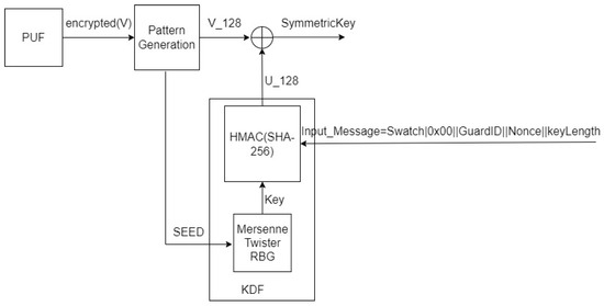
Figure 2.
PUF -based symmetric key generation.
5.2. Online Electronic Lotteries
Online eLotteries represent an application area where the unpredictability of the produced numbers of each draw is an essential requirement. Naturally, in this application field, where high financial stakes exist, more requirements are necessary to ensure the validity of each draw, such as the following:
- The produced numbers should obey the uniform distribution over the required number range.
- It should be infeasible for anyone (even the lottery owner and operator) to predict the numbers of the next draw, given the draw history, with a prediction probability “better” than the uniform over the range of the lottery numbers.
- It should be infeasible for anyone (even the lottery owner and operator) to interfere with the draw mechanism in any way.
- The draw mechanism should be designed so as to obey a number of standards; in addition, there should also be a process through which it can be officially certified (by a lottery designated body) that these standards are met by the lottery operator.
- The draw mechanism should be under constant monitoring (by a lottery designated body) so as to detect and rectify possible deviations from the requirements.
- The details of the operation of the lottery draw mechanism should be publicly available for inspection in order to build trust and interest towards the lottery. In addition, this publicity facilitates auditing (which may be required by a country’s regulation about electronic lotteries).
One such lottery design has been proposed in [19,20]. A high-level description of the system components, as well as their roles, is shown in Figure 3.

Figure 3.
The architecture of the random number generation system.
Generator and Verifier are the two fundamental interacting agents around which the protocol is built. In a high-availability configuration, the Generator can be duplicated, although this is a system-architecture-related decision, not necessary for the protocol we shall discuss.
To enable pair-wise secure communication, the Generator and the Verifier first execute a key-exchange protocol in order to end up sharing a secret key. Additionally, each of them creates a private/public key pair for signing the exchanged communication messages. The Generator then enters an idle state and generates a packet of random numbers only upon the Verifier’s request for the next draw, continuing from the last produced draw.
From the Generator’s pool of truly random bits, drawn from physical sources like semiconductor elements (e.g., shot noise), a series of random bits are chosen as seeds for the deployed software PRNGs. As an alternative, the Generator may use its current internal state to construct the next state deterministically without utilizing any fresh, truly random bits for reseeding the generators. Next, in order to irrevocably link the seed and/or internal state with the coupon file, the Generator combines the drawn genuinely random bits and/or its current state (using the XOR operation) with the hash value of the coupon file. As a result, the coupon file is effectively “frozen”, making it impossible to compare any future, unauthorized modifications to the internal state of the generator, which was committed and signed in the logs at the time in which the draw was initiated.
The Naor–Reingold function (see [35]), which is a one-way pseudorandom function, is then applied to the created bit sequence as a postprocessing safety measure for additional randomization. Then, the software-based random number generators are seeded using this bit sequence. There are currently two block-cipher-based generators (DES and AES) and two cryptographically secure pseudorandom number generators (RSA and BBS) that are utilized in our protocol, but any number of software-based generators can be employed in different output configurations. After that, the Generator signs the numbers generated using the final seed sequence and a bit-commitment mechanism.
On the other side, the Verifier receives the encrypted packet containing the committed to seeds and signed random numbers, and the Generator shuts down. It initially decrypts the received packet in order to obtain the signed numbers, as well as the seed that the Generator is said to have used to generate these numbers. The Verifier then utilizes the seed to replicate the generator’s creation process after confirming that the generator has committed to the provided seed. The draw is deemed successful and is finished by the announcement of the winning numbers if the numbers produced match the numbers supplied by the generator. A process whereby a warning is issued, the draw is canceled and the Verifier starts it again (or takes some other step to ensure integrity and continuity) is enabled if the numbers received do not match the numbers supplied. Notice that the Verifier function performs an audit of the full drawing process, including the independent computation of the hashed version of the participating coupons and the internal generation of truly random bits (seeds).
5.3. The Protocol Components
5.3.1. Prevention of Post-Betting
The ability to detect post-betting, i.e., to detect whether a coupon was placed into the coupon database after the winning numbers were produced by the generators, is an important requirement from the protocol. If such an illegal event is detected, the protocol must be stopped immediately, and the current draw must be canceled without announcing the winning numbers.
This requirement can be easily satisfied by combining information characterizing the state of the coupon file just before the winning numbers are produced. The state can also include information about the truly random seeds obtained from physical sources in order to start the PRNGs of the lottery. For instance, we can use the coupon file’s hash value as the file’s state indicator for ensuring integrity and detecting subsequent, to the draw, efforts to modify it by inserting a new coupon. Then, the hash value of the coupon file along with the used seeds become input to a pseudorandom functions commonly used in cryptography, such as the Naor–Reingold function. In this way, we can also detect insider attacks from corrupted lottery employees who have access to the winning numbers just shortly after they have been generated and before they are announced.
5.3.2. Signing the Numbers and Authenticating Their Source
Both the Generator and the Verifier create, during the lottery initialization process, their own RSA key pair and then exchange their public keys. Using their public keys, they create, jointly, a shared key that they also exchange.
Using the shared secret key, the Generator encrypts the winning numbers and seeds and signs them with its private key. After receiving this signed packet, the Verifier verifies the signature of the Generator and uses the shared key to decrypt the winning numbers and seeds. This encryption and signing process eliminates the risks inherent in authentication methods like verifying IP addresses of servers, exchanging password phrases, etc. As an additional security precaution, the RSA key pairs can be periodically refreshed.
5.3.3. Seed Commitment and Reproduction of Received Numbers
An issue that arises after the reception of the winning numbers of the current draw is whether these numbers were, indeed, generated taking into consideration the coupon file’s hash value in order to avoid post-betting, as we explained earlier.
To accomplish this, the Verifier sends the hash value of the coupon file (the Verifier obtained the coupon file after the betting period closed) to the Generator. Upon reception of the hash value, the Generator draws a seed from the true random number generators, securely combines it with the hash value (e.g., XORs them together) and then commits to the result using the Naor–Reingold (NR for short) function (see [35]). This function is used to process the mixture of seeds derived from the truly random number generators as combined with the hash value of the coupon file. The result of this processing is given as an input to the PRNGs deployed by the lottery (four in the case we study). Moreover, the quality of the seeding process is enhanced; consequently, the overall security of the random number generation protocol is enhanced by the employment of the NR function.
Following this processing, the Generator transmits a bit commitment to the Verifier, and it produces the numbers of the current draw and sends them to the Verifier. Then, the Verifier is able to recreate the numbers using the Generator’s commitment. If the recreated numbers are identical to the received random numbers, then the verification process is successful. In this case, the current draw is considered valid, and the winning numbers can be publicized. Otherwise, an alert is issued for investigating potential malfunction of the generators or an effort to interfere maliciously with the lottery operation.
With respect to the NR function, a key is a tuple , with being P a large prime, Q being a large prime divisor of , g being an element of order Q in and being a uniformly distributed sequence of elements in . Given an input x of n bits, , the NR function is defined as follows:
In the specific implementation in [19,20], the sizes of P and Q were 1000 bits and 200 bits, respectively. Note that in general, a pseudorandom function is applied for both further randomizing the input value and serving as a commitment for the generation of the next winning number sequence, in the case of the lottery. This commitment is based on the Generator’s inputs, i.e., seeds from physical sources and the coupon file’s hash value, so that its output (i.e., winning numbers) can be checked for validity. Since the NR function is pseudorandom, revealing input–output relationships does not affect its security. An alternative approach is the use of another “verifiable (pseudo)random function”, as defined in [36].
Finally, the Simplified Optimal Asymmetric Encryption Padding, or SAEP, protocol (see [37]) can be applied before passing the seeds from the NR function to the Generator. Using this protocol, a padding on the NR function’s output is computed towards security enhancement. More specifically, if M is the message to be encrypted, the SAEP protocol concatenates M with a sequence of 0 s; then, it appends to it a random number r. Then, the hash value of r is computed, XORed with message M and the 0 s. The rmd160 algorithm can be used as the hash function, among other suitable choices. The message that to be encrypted is the concatenation of the result of the XOR operation with random number r. The SAEP protocol is summarized in Figure 4.
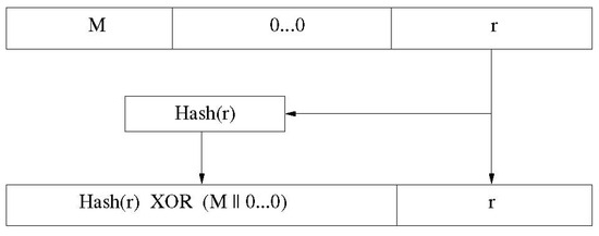
Figure 4.
SAEP protocol.
In the random number generation protocol examined in this section, message M is composed of the seeds that must be sent from the Generator to the Verifier. After the SAEP protocol has been applied, all the information is encrypted and signed with the Generator’s private RSA key. The result of this process is transmitted to the Verifier for the verification process.
Upon the reception of the encrypted and signed packet, the Verifier first validates the signature and then decrypts the message using the shared key. Finally, the Verifier applies the reverse SAEP process, retrieving the commitment (seeds).
Indicative key sizes are 1000 bits for the encryption process and 2000 bits for the signature. The number of 0 s used in the SAEP protocol can be approximately 100. Also, the size of random number r can be approximately 100.
5.3.4. Incorporation of Several True Randomness Sources
The initial randomness, or seed, of a software PRNG must eventually be drawn from a source of true randomness or physical source. After considering the various sources of true randomness within a computer (e.g., /dev/random in LINUX, fluctuations in hard disk access times, motherboard clock frequency drift, etc.) and evaluating the trade-offs between ease of use and quality of output, it was decided to use commercial hardware generators known to pass a number of demanding statistical tests (e.g., Diehard—see Section 4.2 for a brief presentation of the tests).
Moreover, it was important to use several such true randomness sources (see Section 2) with their outputs XORed, since it is not uncommon to have, after some time, risky deviations in the physical characteristics of the devices from which the initial randomness (seed) is drawn. These fluctuations, in turn, may cause the appearance of detectable biases or patterns in the produced number sequences.
5.3.5. Mixing the Outputs of the Generators: Algorithms M and B
As we discussed in Section 3.2.4, algorithm M takes as input two sequences and and combines them in order to produce a sequence of enhanced randomness properties. The algorithm, actually, shuffles the elements of sequence using as indices the elements of sequence . Thus, the elements of the new sequence are the elements of but in different order. Algorithm B is similar to M, but it requires only one sequence as input. The output is, again, a shuffled version of the input sequence.
In the lottery application, however, the involved sequences are composed of 0 s and 1 s; thus, we have implemented slightly different variants of M and B. Now, algorithm M takes as inputs two bit sequences X and Y, while algorithm B takes as input one bit sequence X. In what follows, is the output sequence.
| V[0] = X[0]; V[1] = X[1]; |
| for (j = 2 to length(X) − 1) |
| { |
| i = Y[j]; |
| Xout[j − 2] = V[i]; |
| V[i] = X[j]; |
| } |
| i = Y[0]; |
| Xout[length(X) − 2] = V[i]; |
| V[i] = X[0]; |
| i = Y[1]; |
| Xout[length(X) − 1] = V[i]; |
Algorithm B outputs a sequence of bits with input a sequence of bits X as follows:
| V[0] = X[0]; V[1] = X[1]; |
| for (j = 2 to length(X) − 1) |
| { |
| i = X[j]; |
| Xout[j − 2] = V[i]; |
| V[i] = X[j]; |
| } |
| i = X[0]; |
| Xout[length(X) − 2] = V[i]; |
| V[i] = X[0]; |
| i = X[1]; |
| Xout[length(X) − 1] = V[i]; |
Returning to the generators that the protocol uses, the BBS, RSA/Rabin, DES and AES generators, we can combine them in many ways so that the protocol can swap, periodically and (optionally) unpredictably, to different combinations for the generation of the winning numbers. For instance, at one moment, we can use the BBS and DES generators, combined with the M algorithm and, at a later time, RSA/Rabin with the B algorithm. This makes the lottery protocol more secure and less vulnerable to guessing attacks. Each of the four generators can be used alone or with the B algorithm. In addition, all four generators can be used in groups of two using the M algorithm and in groups of two, three and four using the XOR operation on their outputs.
It was desirable to implement the option of periodically modifying (or through an external signal from the Verifier) the subset of generators whose combined output is used for the lottery draws. This creates additional difficulty to an observer, as the output number sequences originate from different types of generators at different times of the lottery operation.
6. Conclusions
Is it possible to find a method for generating or simulating truly random phenomena, such as a sequence of bits corresponding to the flip of a fair coin, through a systematic procedure or algorithm? According to John von Neumann, this question is contradictory and without meaning, considering anyone who tries to construct random numbers using some algorithmic method is a sinner. The concept of “method” or systematic procedure appears to be incompatible with randomness, at least with respect to a property of randomness that is essential to characterizing a sequence of observations as possessing “randomness”: unpredictability. Through patient observation, the method can be ultimately revealed before the eyes of an observer with sufficient time at her/his disposal, as in the famous game of Eleusis, the game of observation and deductive reasoning. Then, predicting the future workings of the method becomes trivial: just apply the method and obtain its outputs.
What is next, then, even if true randomness does not really exist? The answer lies in the construction of unpredictable, in some precise sense, pseudorandom number generators. The modern science of cryptography, which has its foundations in the science of complexity theory, provides us with tools for building methods that iteratively produce numbers whose observation gives absolutely no evidence of what the subsequent numbers will be, unless an extremely enormous amount of time is expended, which is prohibitive even for the fastest supercomputers that exist today or in the near and far future. In cryptography’s toolbox, we have PRNGs based on the famous RSA public encryption scheme, whose unpredictability is founded on the computational difficulty of the problem of finding prime factors of large integers; the BBS scheme, based on the quadratic residuosity assumption and its computational complexity repercussions; schemes based on other problems, such as that of finding the discrete logarithm in a number field; the AES encryption algorithm; and other “one-way” (i.e., easy to compute but difficult to invert) functions, such as the SHA (Secure Hash Algorithms) class of hash functions.
Based on this context, in this paper, we presented the fundamental concepts behind random number generation processes, as well as the main algorithmic approaches. We fist discussed the crucial concept of entropy as a measure of the strength and quality of both physical and non-physical entropy sources, providing some details with respect to how some recently proposed true random number generators (TRNGs) operate. Then, we discussed how TRNGs can be deployed in applications where algorithms are required for the generation of pseudorandom numbers. These algorithms are called pseudorandom number generators, or PRNGs for short, and deploy TRNGs as entropy sources for producing random seeds. We also discussed the two main classes of PRNGs, the simple linear congruential generators (LCGs), which are predictable in polynomial time given a sufficiently long output, and the cryptographically secure generators, with unpredictability guarantees based on the high computational complexity of some corresponding number theoretical problem on which they are based. Another important aspect of random number generator design is to perform specific randomness tests on the outputs of their implementation. Although it does not hold, in general, that a generator is strong if it passes all the tests, passing the tests is considered a good indication of the generator’s quality. In this context, we covered, in this paper, several widely used statistical tests that can be applied to the outputs of the generators in order to evaluate their “randomness” quality and identify possible structural and/or implementation weaknesses. Finally, we discussed an important application domain of random number generators where the important property is unpredictability, the development and operation of eLotteries. Since, in this application domain, huge financial interests may be at stake if the draw numbers can be guessed, the choice of the supporting random number generators should be based not only on empirical testing but a strong theoretical framework. In this paper, we describe a complete design of an eLottery system that was built and operated for several years in actual eLottery games. We discussed how the different components, such as true random number generators, cryptographically secure generators, seed quality enhancement techniques, post-betting prevention and block ciphers, can be combined towards the generation of long number sequences for which predictability is impossible in practice.
Space limitations, however, do not allow us to continue any further. As a general conclusion, we would like to emphasize that the introduction of computational complexity into application fields such as the generation of random numbers, where the word “method” suggests predictability and order, allows for the implementation of deterministic approaches that although they are, in principle, predictable, they are not so in practice. Thus, we suggest, as a future direction in the random number generation field, the investigation of the interplay between complexity theory and cryptography as foundations of “randomness”.
Author Contributions
Conceptualiztion:, A.B., P.E.N., G.P. and Y.C.S.; methodology, A.B., P.E.N., G.P. and Y.C.S.; formal analysis: A.B., P.E.N., G.P. and Y.C.S.; writing—original draft preparation: P.E.N. and Y.C.S.; writing—review and editing P.E.N. and Y.C.S.; validation, A.B. and G.P. All authors have read and agreed to the published version of the manuscript.
Funding
This research received no external funding.
Data Availability Statement
Not applicable.
Acknowledgments
The work by P.E. Nastou and G. Petroudis was partially supported by the European Regional Development Fund of the European Union and Greek national funds through the Operational Program Competitiveness, Entrepreneurship and Innovation, under the call RESEARCH-CREATE-INNOVATE (project name: SafeIT and project code: T2EDK-01862).
Conflicts of Interest
The authors declare no conflict of interest.
References
- Zenil, H. (Ed.) Randomness through Computation; Collective Volume. World Scientific, 2011. Available online: https://www.worldscientific.com/worldscibooks/10.1142/7973#t=toc (accessed on 24 October 2023).
- Killmann, W.; Schindler, W. A Proposal for Functionality Classes for Random Number Generators. In Proceedings of the Bundesamt Sicherheit der Informationstechnik (BSI), September 2022; Available online: https://www.bsi.bund.de/SharedDocs/Downloads/EN/BSI/Certification/Interpretations/+AIS_31_Functionality_classes_for_random_number_generators_e.pdf?__blob=publicationFile&v=4 (accessed on 24 October 2023).
- Rukhin, A.; Soto, J.; Nechvatal, J.; Smid, M.; Barker, E.; Leigh, S.; Levenson, M.; Vangel, M.; Banks, D.; Heckert, A.; et al. A Statistical Test Suite for Random and Pseudorandom Number Generators for Cryptographic Applications, NIST Special Publication 800-22, Reveision 1a. April 2010. Available online: https://nvlpubs.nist.gov/nistpubs/Legacy/SP/nistspecialpublication800-22r1a.pdf (accessed on 24 October 2023).
- Turan, M.S.; Barker, E.; Kelsey, J.; McKay, K.A.; Baish, M.L.; Boyle, M. Recommendation for the Entropy Sources Used for Random Bit Generation, NIST Special Publication 800-90B. January 2018. Available online: https://doi.org/10.6028/NIST.SP.800-90B (accessed on 24 October 2023).
- Marsaglia, G. The Marsaglia Random Number CDROM including the Diehard Battery of Tests of Randomness. Florida State University, 1995. Available online: https://web.archive.org/web/20160125103112/http://stat.fsu.edu/pub/diehard/ (accessed on 25 January 2016).
- Cachin, C. Entropy Measures and Unconditional Security in Cryptogrphy. Diss. ETH No. 12187. Ph.D. Thesis, ETH Zurich, Zurich, Switzerland, 1997. [Google Scholar]
- Barker, E.; Kelsey, J.; McKay, K.; Roginsky, A.; Turan, M.S. Recommendation for Random Bit Generation (RBG) Constructions. NIST Special Publication 800-90C Revision 3. September 2022. Available online: https://doi.org/10.6028/NIST.SP.800-90C.3pd (accessed on 24 October 2023).
- Viega, J.; Messier, M. Secure Programming Cookbook for C and C++: Recipes for Cryptography, Authentication, Input Validation and More; O’Reilly Media: Sebastopol, CA, USA, 2003. [Google Scholar]
- Chen, T.; Ma, Y.; Lin, J.; Cao, Y.; Liv, N.; Jing, J. A Lightweight Full Entropy TRNG with On-Chip Entropy Assurance. IEEE Trans. Comput. Aided Des. Integr. Circuits Syst. 2021, 40, 2431–2444. [Google Scholar] [CrossRef]
- Prada-Delgado, M.A.; Martinez-Gomez, C.; Baturone, I. Auto-Calibrated Ring Oscillator TRNG Based on Jitter Accumulation. In Proceedings of the 2020 IEEE International Symposium on Circuits and Systems (ISCAS), Seville, Spain, 12–14 October 2020. [Google Scholar]
- Danesh, M.; Venkatasubramaniyan, A.B.; Kappor, G.; Ramesh, N.; Sadasivuni, S.; Chandrasekaran, S.T.; Sanyal, A. Unified Analog PUF and TRNG Based on Current-Steering DAC and VCO. IEEE Trans. Very Large Scale Integr. (VLSI) Syst. 2020, 28, 2280–2289. [Google Scholar] [CrossRef]
- Zhao, J.; Chen, B.; Wang, W.; Xia, W.; Ye, J.; Bi, H.; Cao, J.; Jin, C.; Yu, X.; Han, G.; et al. A True Random Number Generator Based on Semiconductor-Vacancies Junction Entropy Source and Square Transform Method. IEEE Trans. Electron Devices 2023, 70, 5484–5488. [Google Scholar] [CrossRef]
- Fu, S.; Li, T.; Zhang, C.; Li, H.; Ma, S.; Zhang, J.; Zhang, R.; Wu, L. RHS-TRNG: A Resilient High-Speed True Random Number Generator Based on STT-MTJ Device. IEEE Trans. Very Large Scale Integr. (VLSI) Syst. 2023, 31, 1578–1591. [Google Scholar] [CrossRef]
- Guajardo, J.; Kumar, S.S.; Schrijen, G.J.; Tuyls, P. FPGA Intrinsic PUFs and Their Use for IP Protection. In Proceedings of the Cryptographic Hardware and Embedded Systems—CHES 2007: 9th International Workshop, Vienna, Austria, 10–13 September 2007; pp. 63–80. [Google Scholar]
- O’Donnell, C.W.; Suh, G.E.; Devadas, S. PUF-Based Random Number Generation. MIT CSAIL CSG Tech. Memo 2004, 481. [Google Scholar]
- Cao, Y.; Liu, W.; Qin, L.; Liu, B.; Chen, S.; Ye, J.; Xia, X.; Wang, C. Entropy Sources Based on Silicon Chips: True Random Number Generator and Physical Unclonable Function. Entropy 2022, 24, 1566. [Google Scholar] [CrossRef] [PubMed]
- Blum, M.; Micali, S. How to Generate Cryptographically Strong Sequences of Pseudo-Random Bits. Siam Comput. 1984, 13, 850–864. [Google Scholar] [CrossRef]
- Yao, A. Theory and Applications of Trapdoor Functions. In Proceedings of the 23rd Annual Symposium on Foundations of Computer Science (SFCS 1982), Chicago, IL, USA, 3–5 November 1982. [Google Scholar]
- Konstantinou, E.; Liagkou, V.; Spirakis, P.; Stamatiou, Y.C.; Yung, M. Electronic National Lotteries. In Lecture Notes in Computer Science, Proceedings of the Financial Cryptography: 8th International Conference, FC 2004, Key West, FL, USA, 9–12 February 2004; Springer: Berlin/Heidelberg, Germany, 2004; Volume 3110, pp. 147–163. [Google Scholar]
- Konstantinou, E.; Liagkou, V.; Spirakis, P.; Stamatiou, Y.C.; Yung, M. “Trust Engineering:” From Requirements to System Design and Maintenance—A Working National Lottery System Experience. In Lecture Notes in Computer Science, Proceedings of the Information Security, ISC 2005, Singapore, 20–23 September 2005; Springer: Berlin/Heidelberg, Germany, 2004; Volume 3650, pp. 44–58. [Google Scholar]
- Goldreich, O.; Goldwasser, S.; Micali, S. How to construct random functions (extended abstract). In Proceedings of the 25th Annual Symposium on Foundations of Computer Science, West Palm Beach, FL, USA, 24–26 October 1984; pp. 464–479. [Google Scholar]
- Knuth, D. The Art of Computer Programming. Volume 2, Seminumerical Algorithms, 3rd ed.; Addison-Wesley Professional: Sebastopol, CA, USA, 1997. [Google Scholar]
- Boyar, J. Inferring sequences produced by pseudo-random number generators. J. Assoc. Comput. Mach. 1989, 36, 129–141. [Google Scholar] [CrossRef]
- Boyar, J. Inferring sequences produced by a linear congruential generator missing low-order bits. J. Cryptol. 1989, 1, 177–184. [Google Scholar] [CrossRef]
- Kranakis, E. Primality and Cryptography; Wiley-Teubner Series in Computer Science: Hoboken, NJ, USA, 1986. [Google Scholar]
- Blum, L.; Blum, M.; Shub, M. A Simple Unpredictable Pseudo-Random Generator. SIAM J. Comput. 1986, 15, 364–383. [Google Scholar] [CrossRef]
- Carmichael, R.D. On composite numbers P which satisfy the Fermat congruence aP−1 ≡ 1 mod P. Am. Math. Mon. 1919, 26, 137–146. [Google Scholar]
- Alexi, W.; Chor, B.; Goldreich, O.; Schnorr, C. RSA and Rabin Functions: Certain Parts are as Hard as the Whole. SIAM J. Comput. 1988, 17, 194–209. [Google Scholar] [CrossRef]
- Shparlinski, I. On the linear complexity of the power generator. Des. Codes Cryptogr. 2001, 23, 5–10. [Google Scholar] [CrossRef]
- Mcrypt Cryptographic Library. Available online: ftp://mcrypt.hellug.gr/pub/crypto/mcrypt (accessed on 24 October 2023).
- Kelsey, J.; Schneier, B.; Ferguson, N. Yarrow-160: Notes on the Design and Analysis of the Yarrow Cryptographic Pseudorandom Number Generator. In Sixth Annual Workshop on Selected Areas in Cryptography; Springer: Berlin/Heidelberg, Germany, 1999. [Google Scholar]
- Koçak, O.O.; Sulak, F.; Doğanaksoy, A.; Uğuz, M. Modifications of Knuth Randomness Tests for Integer and Binary Sequences. Commun. Fac. Sci. Univ. Ank. Ser. Math. Stat. 2018, 67, 64–81. [Google Scholar]
- Barker, E.; Roginsky, A.; Davis, R. Recommendation for Cryptographic Key Generation. NIST Special Publication 800-133 Revision 2. June 2020. Available online: https://doi.org/10.6028/NIST.SP.800-133r2 (accessed on 24 October 2023).
- Barker, E.; Kelsey, J. Recommendation for Random Number Generation Using Deterministic Random Bit Generators. NIST Special Publication 800-90A Revision 1. June 2015. Available online: https://doi.org/10.6028/NIST.SP.800-90Ar1 (accessed on 24 October 2023).
- Naor, M.; Reingold, O. Number-theoretic constructions of efficient pseudo-random functions. In Proceedings of the 38th IEEE Symposium on Foundations of Computer Science, Miami Beach, FL, USA, 19–22 October 1997. [Google Scholar]
- Micali, S.; Rabin, M.; Vadhan, S. Verifiable Random Functions. In Proceedings of the 40th Annual Symposium on the Foundations of Computer Science (FOCS ‘99), New York, NY, USA, 17–18 October 1999; pp. 120–130. [Google Scholar]
- Boneh, D. Simplified OAEP for the RSA and Rabin functions. In Lecture Notes in Computer Science, Crypto 2001; Springer: Berlin/Heidelberg, Germany, 2001; Volume 2139, pp. 275–291. [Google Scholar]
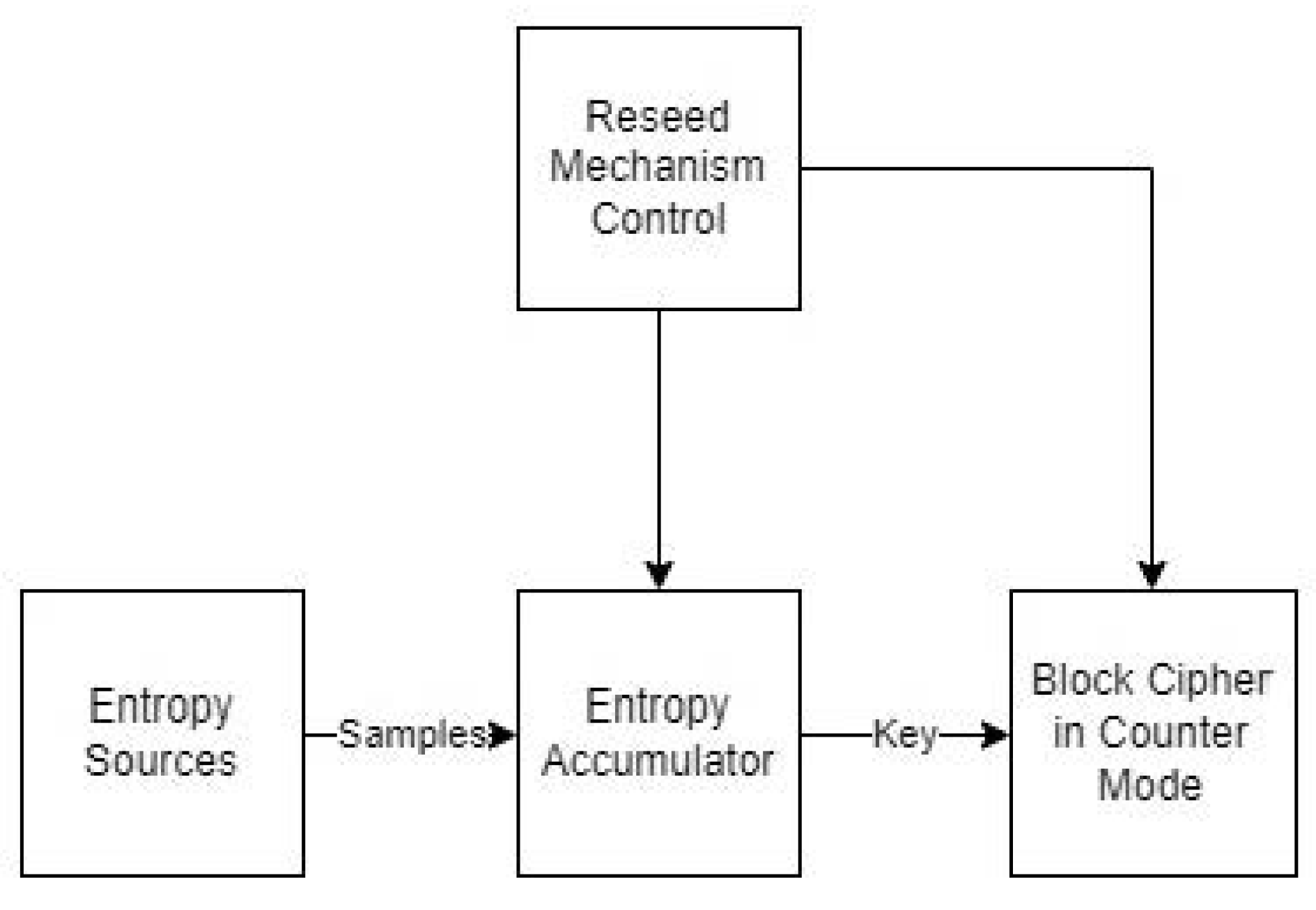
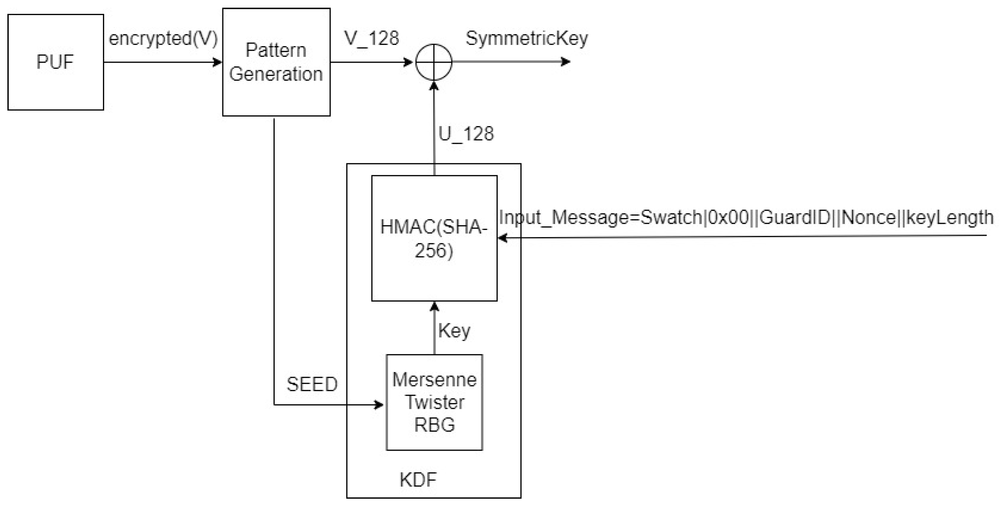
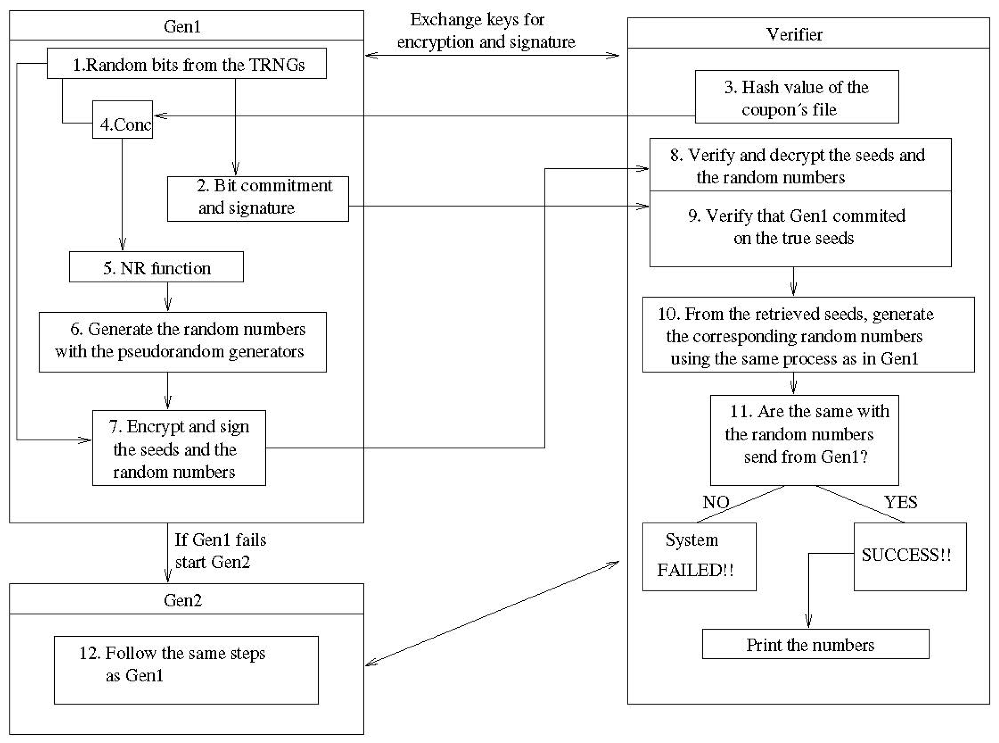
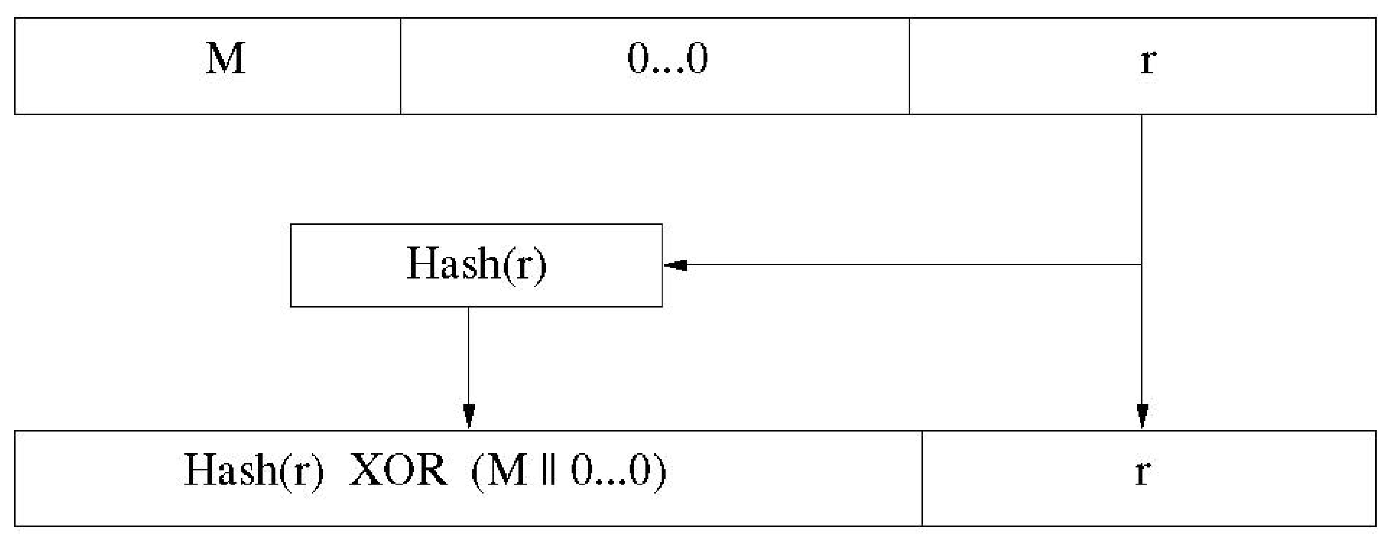
Disclaimer/Publisher’s Note: The statements, opinions and data contained in all publications are solely those of the individual author(s) and contributor(s) and not of MDPI and/or the editor(s). MDPI and/or the editor(s) disclaim responsibility for any injury to people or property resulting from any ideas, methods, instructions or products referred to in the content. |
© 2023 by the authors. Licensee MDPI, Basel, Switzerland. This article is an open access article distributed under the terms and conditions of the Creative Commons Attribution (CC BY) license (https://creativecommons.org/licenses/by/4.0/).