5.1. Data
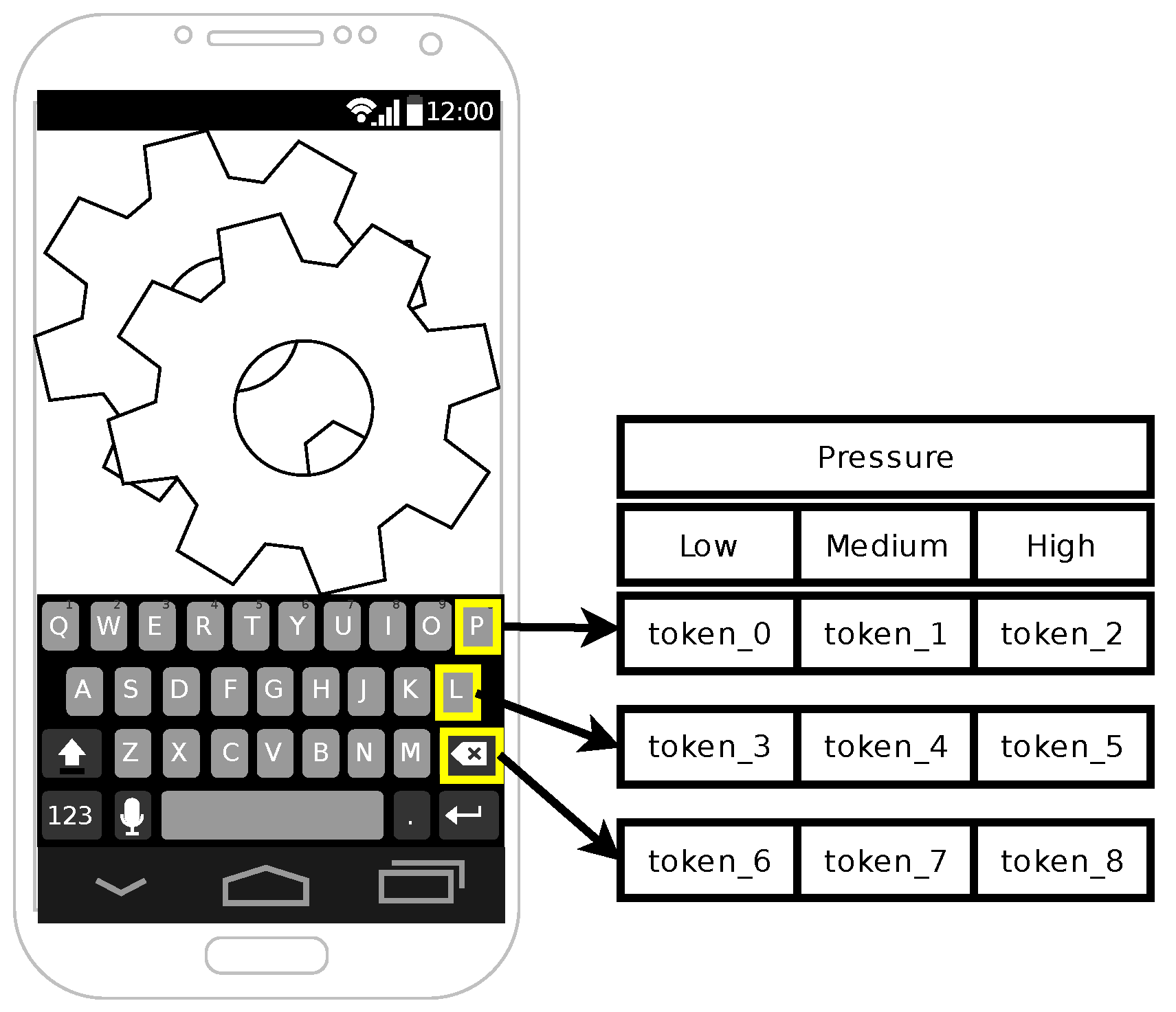
Software keyboard interactions result in data derived from user–application interactions. Each interaction creates a MotionEvent object in the Android framework. A MotionEvent object contains a variety of information about the touch event—pressure, location of touch, and time—a subset of which is used in model generation.
MotionEvent touch pressure fidelity is device-dependent. Pressure value range and resolution vary. This variation might result from physical sensors or hardware drivers. Nexus 7 tablets, used in this work, provide high fidelity pressure measurements. Pressure ranges from to in steps of .
We modified a software keyboard application to collect MotionEvent objects. Four users completed at least 5000 interactions on three Nexus 7 tablets. This gives us 12 distinct (user, device) data sets. One additional user generated a similar data set on only one device, leading to an overall count of 13 distinct data sets. Users played two typing games. One game from Google Play Store, Typeracer, provides random quotes from books and poems. It is designed for typing practice. In our context, this provides a diverse set of dictionaries for user profile generation, modeling multiple app experiences. A similar second game, Typing Champ, from Google Play Store was also used. However, it presents only single words from a dictionary rather than phrases as in Typeracer.
5.3. Comparing Profiles—Divergence
User profiles are sets of
n-grams with frequency vectors. An
n-gram
consists of a window of
token sequence
W along with a successor frequency vector
v represented as
. The successor frequency vector captures the transition frequency from
W to all possible tokens in the token alphabet
—the result of tokenization described earlier.
(
) refers to the window (vector) component of the
n-gram
. An
n-gram
occurs with frequency
in a user profile
computed as
. Equation (
2) defines a profile divergence; it is a weighted sum of next token probability differences.
is the divergence between profiles B and P, or more accurately, divergence of B from P.
is the divergence between n-grams and .
We define a search function to denote the n-gram with window W in profile P. If an n-gram with window W does not exist in profile P, this function returns a null n-gram with vector .
Interaction profile B is authenticated against user profile P. An interaction profile B is generated from a set of recent keyboard transaction touch events. A user profile P is a model of a user’s touch keyboard interactions. For each n-gram in B, takes the divergence between and its twin n-gram in profile P given by . This divergence between n-grams, , is further weighted by the frequency of in B. Note that this weight selection from profile B makes this divergence metric asymmetric.
computes the divergence over all transitions or entries in the vector
, which is computed as absolute value
which is further weighted by the frequency of the transition on token
leading to
. This expression is summed up over each token
.
The divergence ranges from to ; it describes how much the interaction profile B deviates or diverges from user profile P. is maximally close.
Order matters—. The former compares n-grams in a user profile P to equivalent n-grams in an interaction profile B, whereas the latter compares an interaction profile B against a user profile P. Note that each summand in the divergence computation is multiplied by the frequency of that in the first argument profile of D. If a given n-gram is not in the first argument profile, its frequency is zero. Hence, regardless of the frequency of that in the second argument profile, it will be suppressed, not counted, in the divergence computation. A side-effect of this usually is that many n-grams in a user profile do not contribute to the divergence for the following reason. Usually the user profile would contain many more n-grams than an interaction profile, since a user profile is built over multiple contexts and sessions, whereas an interaction profile is typically from a single session.
Note that our divergence definition is based on the notion of statistical divergence between two probability distributions on the same probability space
. Kullback–Leibler divergence [
39] is a good example of this concept. For two discrete probability distributions
,
, Kullback–Leibler divergence is defined as
. There is a similar definition with an integral for continuous probability distributions. Note that since this is a weighted sum with
; it is asymmetric. This also motivates our use of
weight in Equation (
2). In addition, note that in computing
P’s divergence from
Q, if
is zero for some probability space element
x, the corresponding element
x in
, even with
, is not counted. This is akin to not counting the
n-grams in user profile
P if the corresponding
n-gram does not exist in the interaction profile
B.
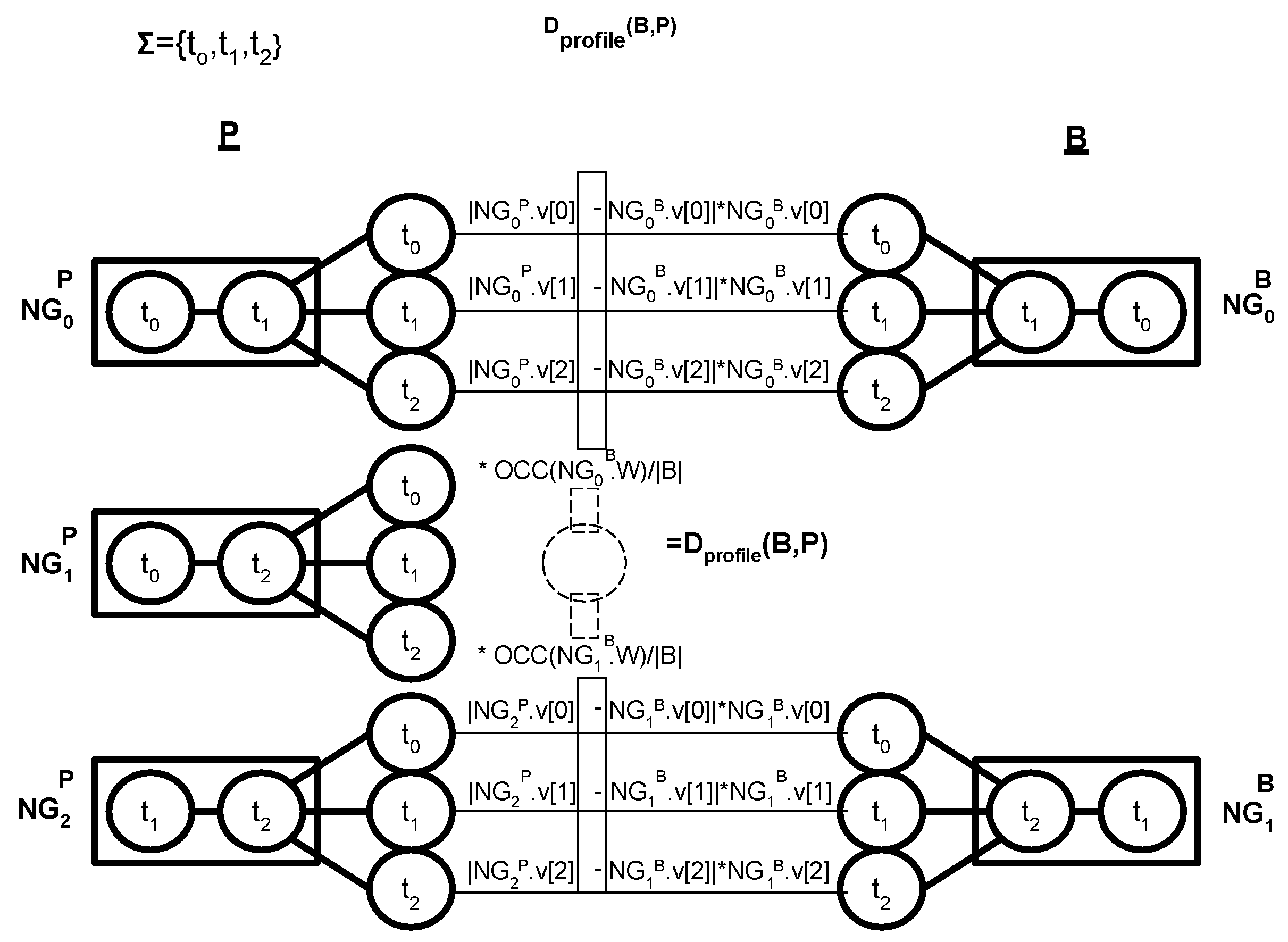
Figure 6 computes
. The left side of the figure shows 3-grams in a user profile
P. The right side shows 3-grams from an interaction profile
B. For this example,
. The top left 3-gram
in user profile
P has a window
with a successor vector
. Similarly, the 3-gram
in the top right of the figure from the interaction profile
B has the same window
and a successor vector
. Hence, in the divergence computation for
, there will be a term for
. That term expands into difference terms by each successor token, resulting in Axis-0 difference term
. However, this difference is further weighted by the probability of Axis-0 in the interaction profile
B’s successor vector captured by
. This leads to the weighted Axis-0 difference term
. This results in the weighted average difference of
. However, this term is further weighted by the frequency of window
in the interaction profile
B. If
follows
in the interaction strings for
B times,
follows
in the interaction strings for
B times, and
follows
in the interaction strings for
B times, the total count of
occurrences is
. The relative frequency of
in
B is
. This will lead to the term
.
The computation excludes the 3-gram in P from this divergence computation since the corresponding 3-gram window does not exist in the interaction profile B. This demonstrates profile divergence computation asymmetry.
Authentication,
, compares an interaction profile
B against a user profile
P. Authentication compares
against a threshold profile divergence value.
5.5. Comparing Profiles—Machine Learning
Machine learning provides an alternative profile comparison method to the divergence measure. It uses a set of features to predict a class. Training a machine learning classifier involves providing a set of feature vectors with known classes for supervised learning. Unsupervised learning techniques do not use class labels. Instead, they create clusters of associated feature vectors. We use supervised machine learning classification schemes.
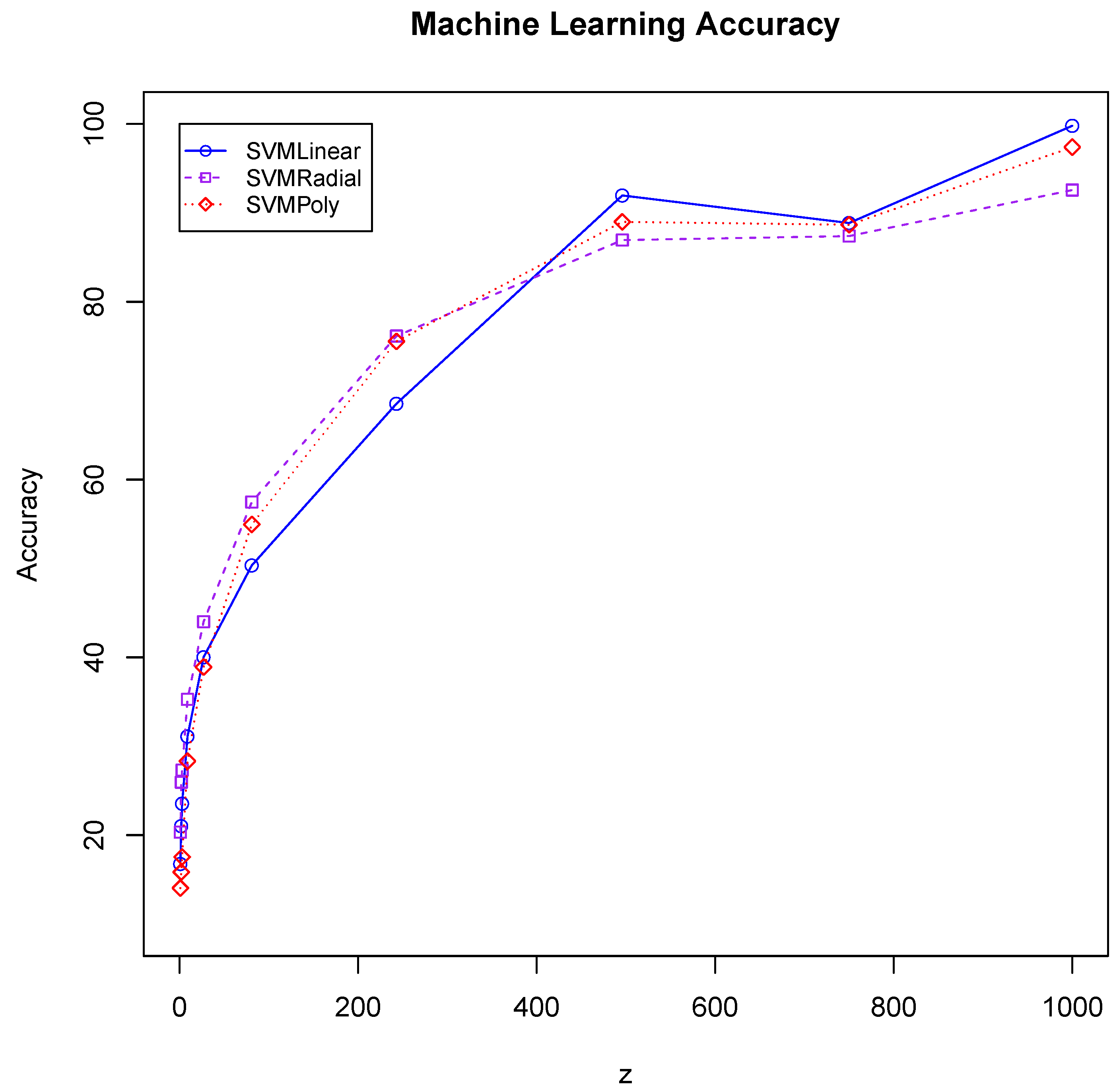
Raw (location, pressure) data are mapped to machine learning features using a z-sequence scheme. Raw input sequences are parsed into all z-sized subsequences—similar to the n-gram sliding window. is the ith raw data sequence element having location () and pressure () values. A 1-sequence provides the machine learning classifier with features (, ) and a class that is the combined user–device identity similar to user profile P. The 2-sequence features are (, , , ). Likewise, z-sequence features are (, , , , …, , ). Providing a z-sequence allows machine learning classifiers to make predictions based on input token sequences.
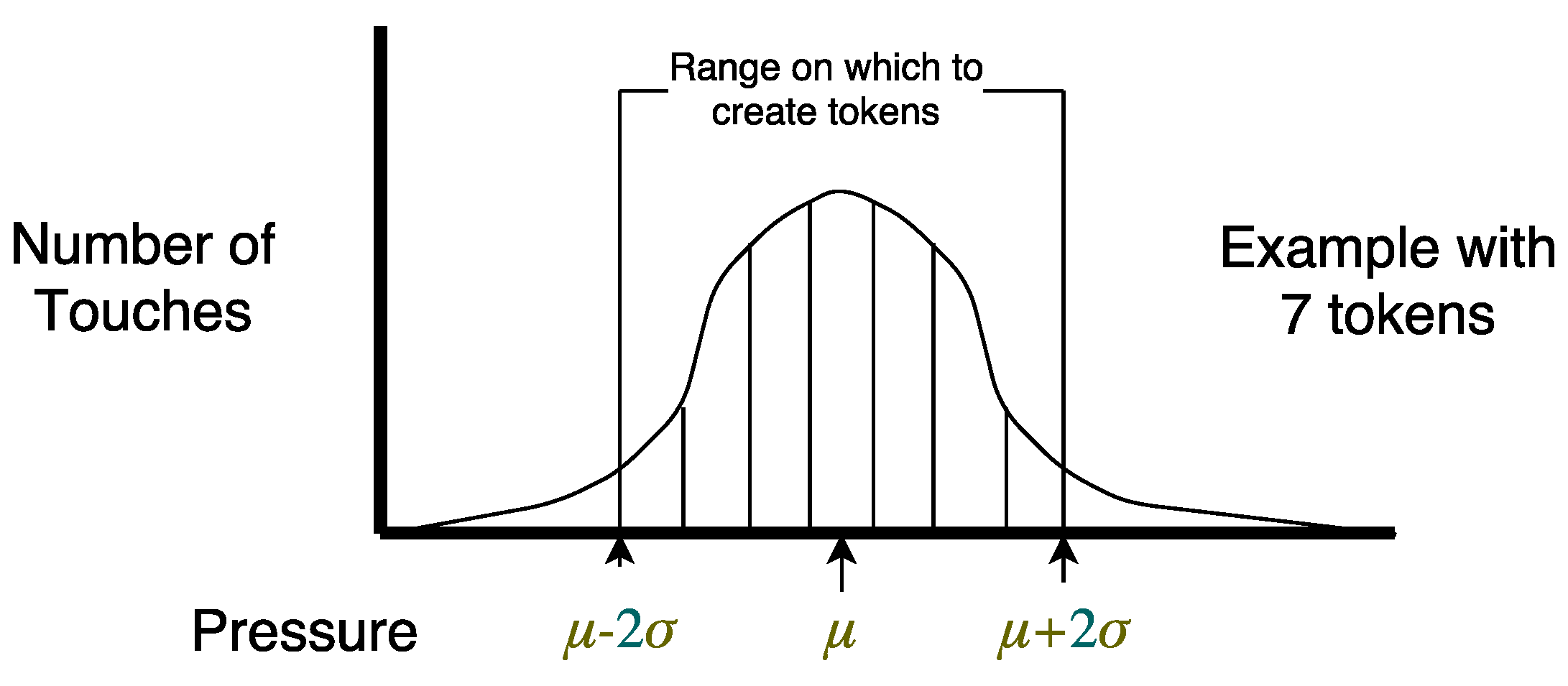
Our divergence measure utilizes statistical techniques to map pressure values to tokens. Following this, probabilities for each
n-gram and each token succeeding that
n-gram window are computed. Analogous tokenized data are provided to machine learning classifiers for a fair comparison against our divergence metric. We employ a second
z-sequence scheme with raw pressure values transformed into token indexes. These token indexes correspond to the
range containing the pressure value. These ranges are discussed in
Section 5. In another scheme, we provide the machine learning classifier with
n-gram frequency and successor vector as well.
Table 2 summarizes these schemes.
