
Grid Cyber-Security Strategy in an Attacker-Defender Model †


Abstract
:1. Introduction
2. Terminology
2.1. Basic Definitions in Probability Theory
2.2. Basic Definitions in Game Theory
- a collection of decision-makers, called players;
- the possible information states of each player at each decision time;
- the collection of feasible moves (decisions, actions, etc.) that each player can choose to make in each of his possible information states;
- a procedure for determining how the move choices of all the players collectively determine the possible outcome of the game; and
- preferences of the individual players over these possible outcomes, typically measured by a utility or payoff function.
3. Background and Prior Work
4. Attack Scenarios
4.1. Single-Layer Parallel PLADD System
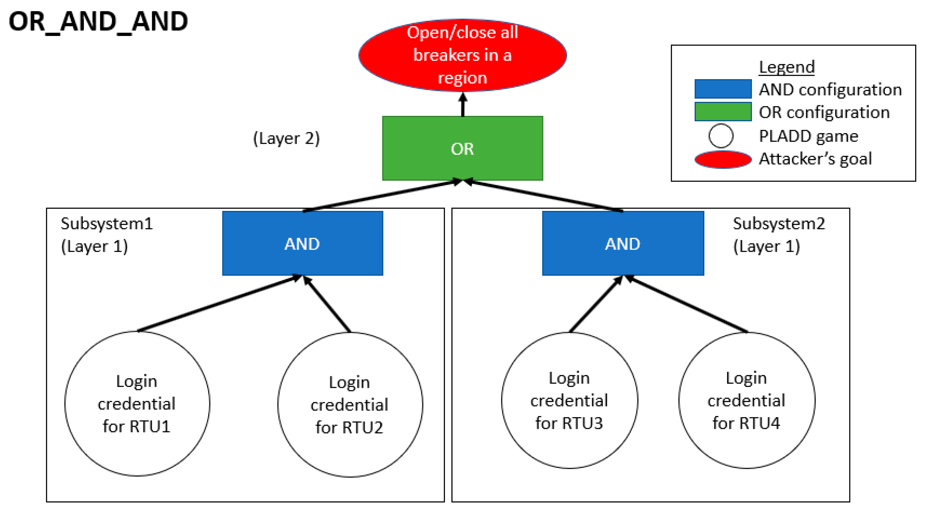
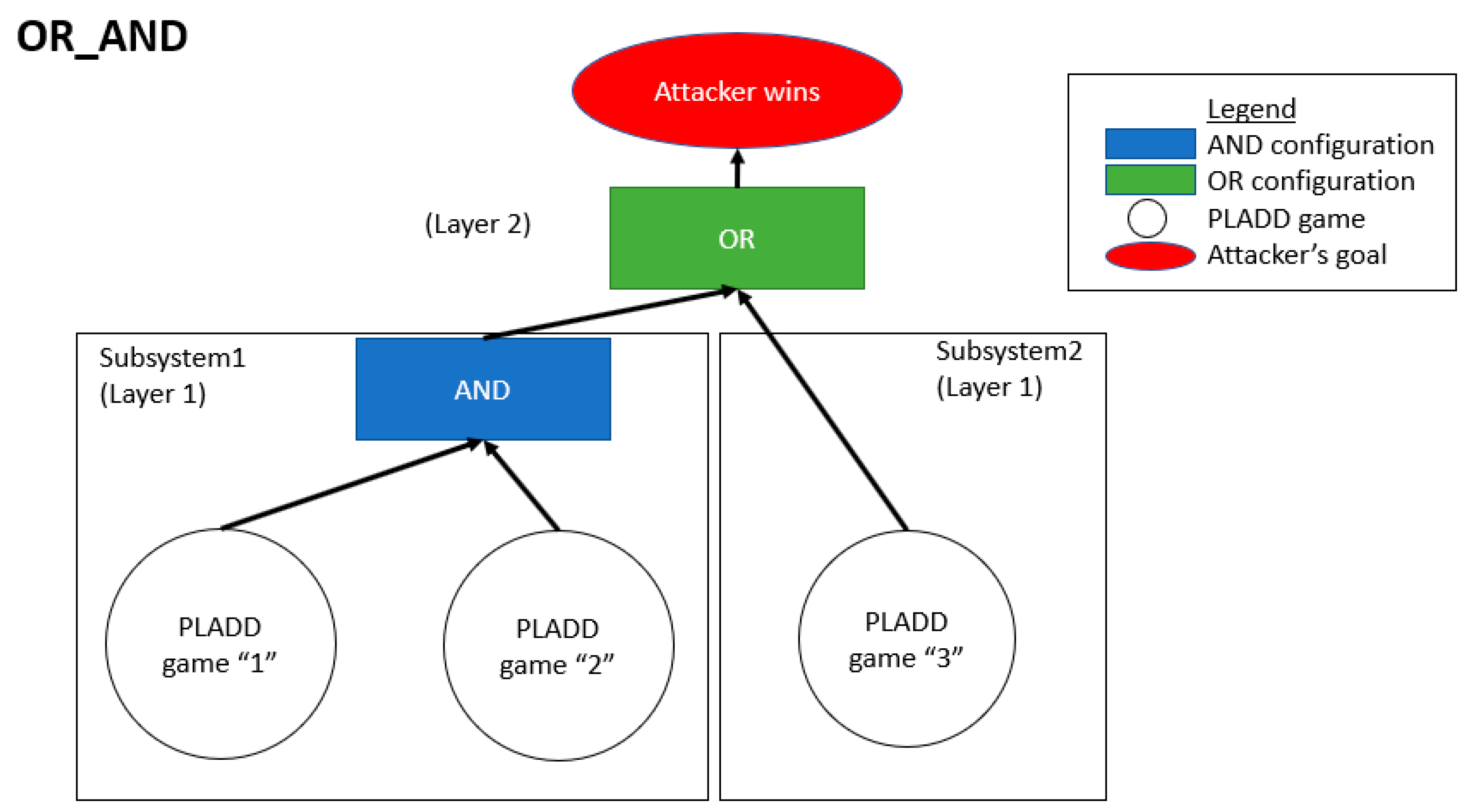
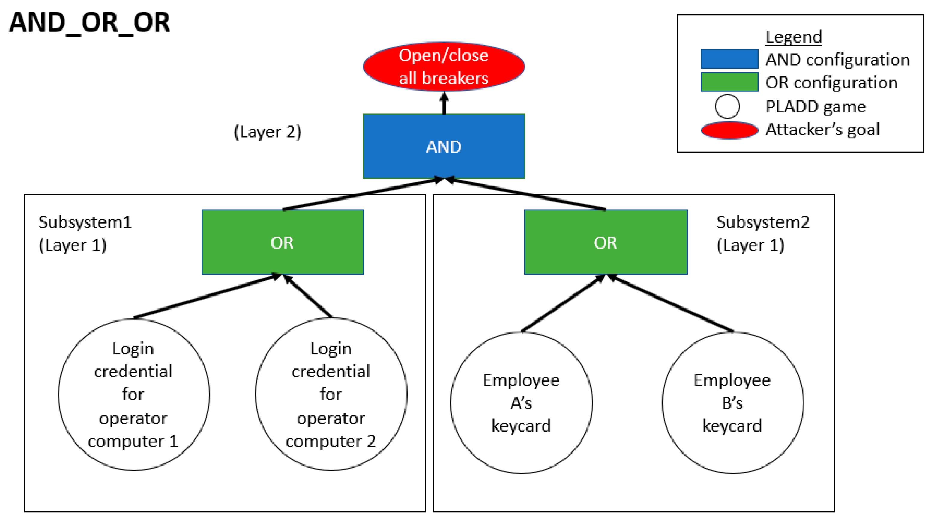
4.2. Hierarchical Parallel PLADD System
5. Mathematical Model Basics
5.1. Notation and Definitions
5.2. Single PLADD Game
- (a)
- The defender executes “take” moves periodically; specifically, the defender executes “take” moves at {}.
- (b)
- is less than
- (c)
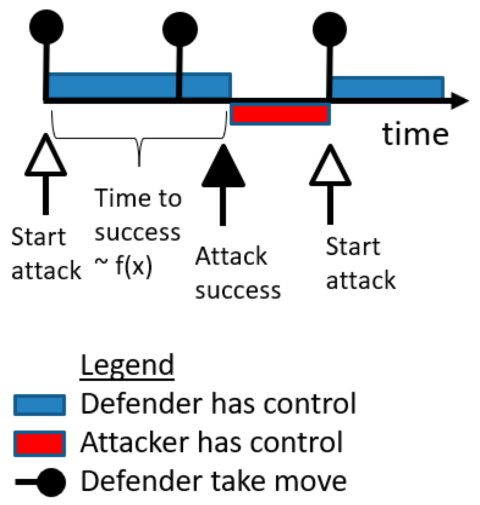
- The attacker is persistent, i.e., starts an attack at time 0 and immediately after anytime the defender takes back the resource.
6. Overview of Major Theorems
6.1. Single-Layer Parallel PLADD System
6.2. Hierarchical Parallel PLADD System
- The resets of each PLADD game in the hierarchical parallel PLADD system are at the same time.
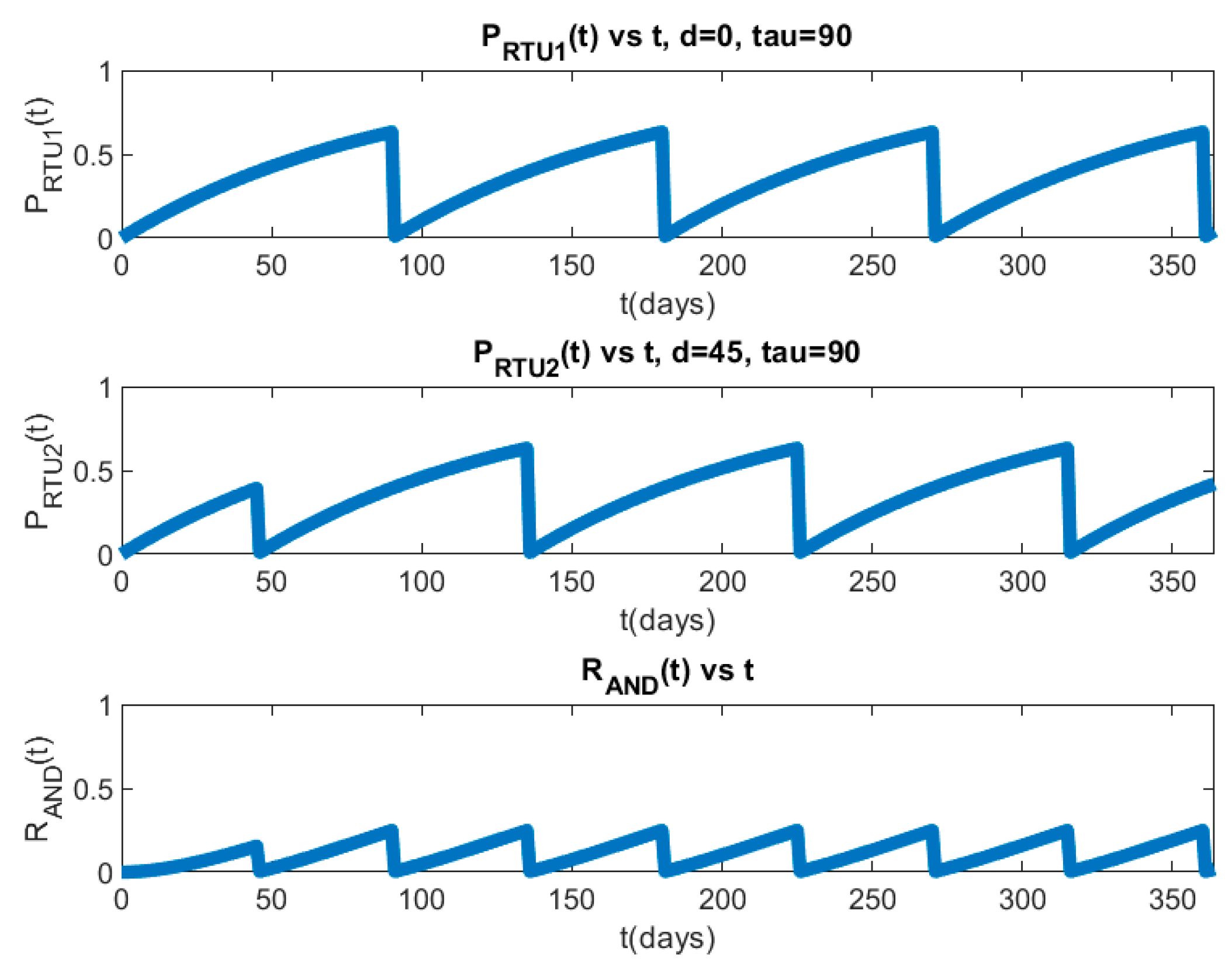
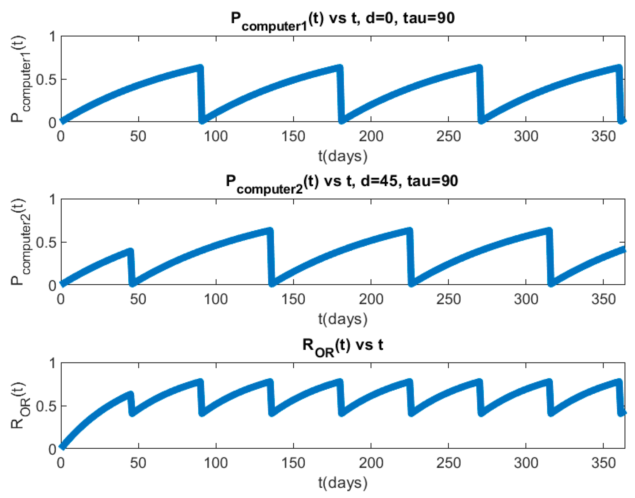
- The resets of each PLADD game in subsystem 1 are at the same time, and the PLADD game in subsystem 2 is offset by 45, which is .
- The resets of each PLADD game in subsystem 1 are offset by 0 and 45, and the PLADD game in subsystem 2 is offset by 0.
- The resets of each PLADD games in subsystem 1 are offset by 0 and 45, and the PLADD game in subsystem 2 is offset by 45.
- The resets of each PLADD game in the hierarchical parallel PLADD system are at the same time.
- The resets of each PLADD game in subsystem 1 are at the same time, and the PLADD game in subsystem 2 is offset by 45, which is .
- The resets of each PLADD game in subsystem 1 are offset by 0 and 45, and the PLADD game in subsystem 2 is offset by 0.
- The resets of each PLADD game in subsystem 1 are offset by 0 and 45, and the PLADD game in subsystem 2 is offset by 45.
7. Mathematical Model in Detail
7.1. Single PLADD Game
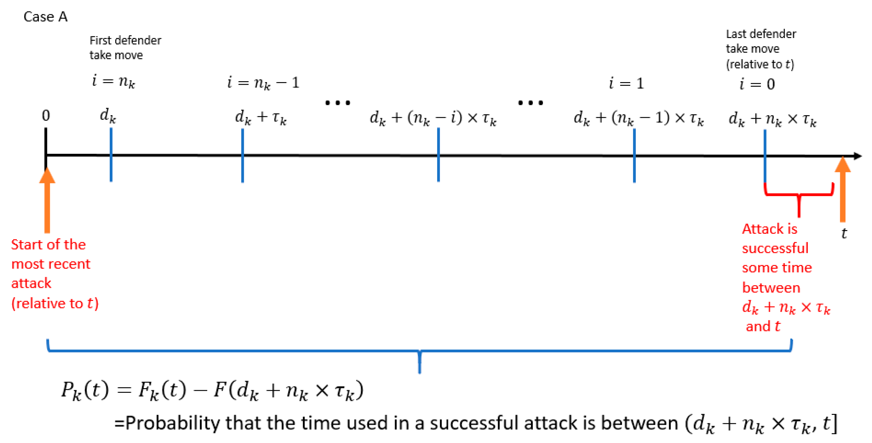
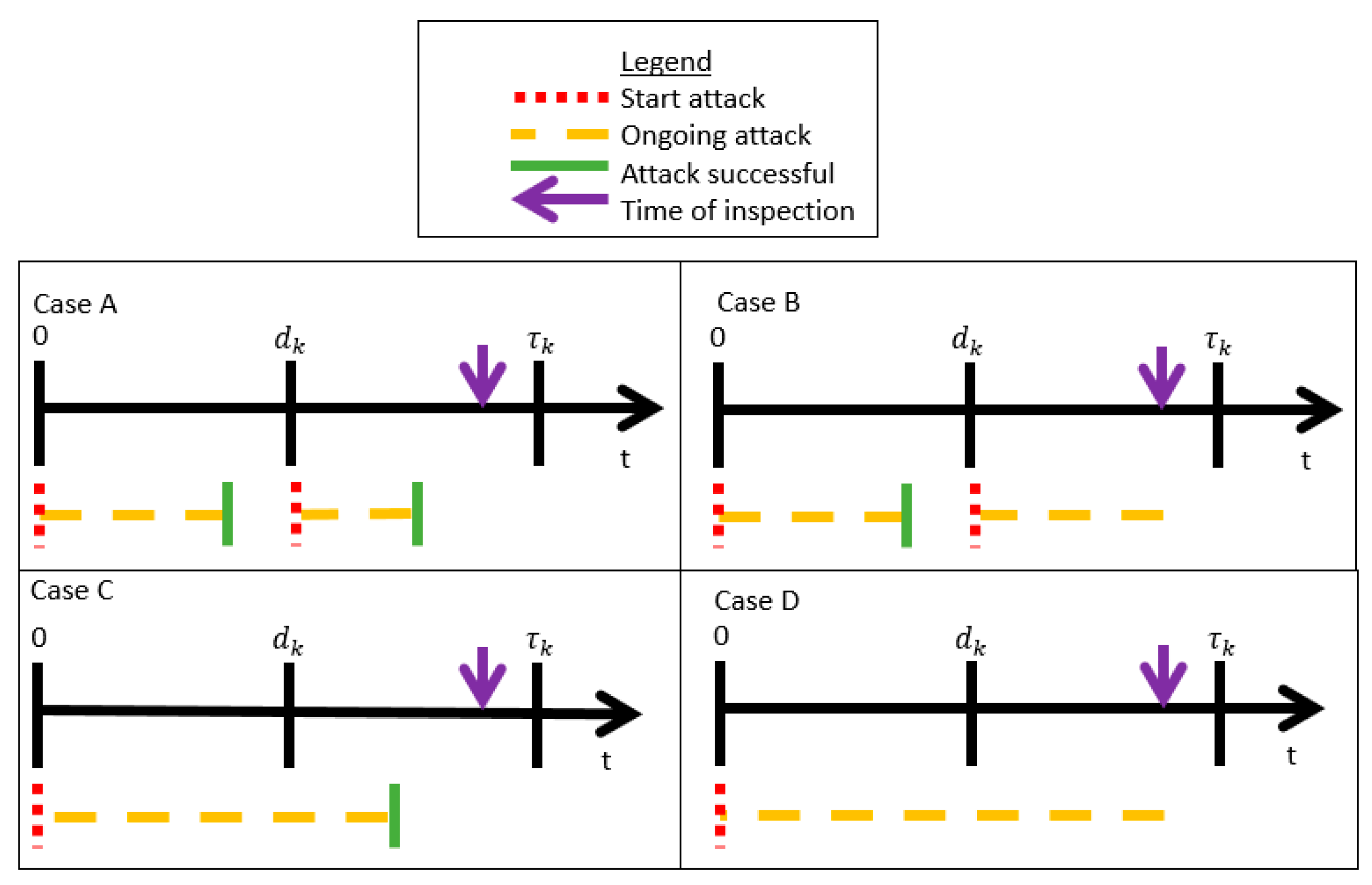
- The probability that the attacker controls the resource at time (which is the time of the attacker′s most recent attack relative to ).
- The probability that the time used in a successful attack is within the range .
- is the start time of the attacker′s most recent attack relative to the variable .
- is the amount of time between the start time of the attacker′s most recent attack relative to the variable .
- is the time of the last defender “take” move relative to the variable .
- is the amount of time between the start of the attacker′s most recent attack relative to the time of the last defender “take” move.
- is the probability that the attacker controls the resource at .
- is the probability that the time used in a successful attack is less than or equal to .
- is the probability that the time used in a successful attack is less than or equal to .
- is the probability that the time used in a successful attack is between (, ].
7.2. Parallel PLADD System
8. Experimental Results
8.1. Single-Layer PLADD Simulation
8.2. Hierarchical PLADD Simulation
9. Discussion
10. Conclusions
Author Contributions
Funding
Data Availability Statement
Conflicts of Interest
References
- Chen, Y.; Mooney, V.; Grijalva, S. Grid Cyber-Security Strategy in an Attacker-Defender Model. In Proceedings of the 2020 Clemson University Power Systems Conference (PSC), Clemson, SC, USA, 10–13 March 2020; pp. 1–8. [Google Scholar] [CrossRef]
- Strengthening the Cybersecurity of Federal Networks and Critical Infrastructure. Available online: https://www.energy.gov/sites/prod/files/2018/05/f51/EO13800%20electricity%20subsector%20report.pdf (accessed on 26 December 2020).
- Lee, R.M.; Assante, M.J.; Conway, T. Analysis of the Cyber Attack on the Ukrainian Power Grid. 2016. Available online: https://ics.sans.org/media/E-ISAC_SANS_Ukraine_DUC_5.pdf (accessed on 26 December 2020).
- Styczynski, J. When the Lights Went Out. Available online: https://www.boozallen.com/content/dam/boozallen/documents/2016/09/ukraine-report-when-the-lights-went-out.pdf (accessed on 26 December 2020).
- Chukwuka, V.; Chen, Y.; Grijalva, S.; Mooney, V. Bad Data Injection Attack Propagation in Cyber-Physical Power Delivery Systems. In Proceedings of the 2018 Clemson University Power Systems Conference (PSC), Charleston, SC, USA, 4–7 September 2018; pp. 1–8. [Google Scholar] [CrossRef]
- Dario, B. Game Theory: Models, Numerical Methods and Applications. Found. Trends® Syst. Control 2014, 1, 379–522. [Google Scholar]
- Deisenroth, M.P.; Faisal, A.A.; Ong, C.S. Mathematics for Machine Learning: Cambridge University Press. Available online: https://mml-book.github.io/book/mml-book.pdf (accessed on 28 December 2020).
- John the Ripper Password Cracker. Openwall. Available online: https://www.openwall.com/john/ (accessed on 15 November 2019).
- Ulrich, J.; Drahos, J.; Govindarasu, M. A symmetric address translation approach for a network layer moving target defense to secure power grid networks. In Proceedings of the 2017 Resilience Week (RWS), Wilmington, DE, USA, 18–22 September 2017; pp. 163–169. [Google Scholar] [CrossRef]
- Evtyushkin, D.; Ponomarev, D.; Abu-Ghazaleh, N. Jump over ASLR: Attacking branch predictors to bypass ASLR. In Proceedings of the 2016 49th Annual IEEE/ACM International Symposium on Microarchitecture (MICRO), Taipei, Taiwan, 15–19 October 2016; pp. 1–13. [Google Scholar] [CrossRef]
- Hashcat-Advanced Password Recovery. Hashcat. Available online: https://hashcat.net/hashcat/ (accessed on 15 November 2019).
- Bošnjak, L.; Sreš, J.; Brumen, B. Brute-force and dictionary attack on hashed real-world passwords. In Proceedings of the 2018 41st International Convention on Information and Communication Technology, Electronics and Microelectronics (MIPRO), Opatija, Croatia, 21–25 May 2018; pp. 1161–1166. [Google Scholar] [CrossRef]
- Jones, S.; Outkin, A.; Gearhart, J.; Hobbs, J.; Siirola, J.; Phillips, C.; Verzi, S.; Tauritz, D.; Mulder, S.; Naugle, A. Evaluating Moving Target Defense with PLADD. Available online: https://prod-ng.sandia.gov/techlib-noauth/access-control.cgi/2015/158432r.pdf (accessed on 29 December 2020).


| Notation | Definition |
|---|---|
| ℕ | Natural numbers (1, 2, 3, 4, etc.). |
| The number of PLADD games in parallel PLADD system. | |
| The index of a PLADD game in parallel PLADD system; note that | |
| Time; we allow time to begin at 0 and proceed to infinity. | |
| The defender “take” period of a single game with index k in a parallel PLADD system. | |
| The time of occurrence of the first defender ““take” move in a game with index k in a parallel PLADD system. A “take” move resets control to the defender. | |
| The probability density function of the attacker′s time-to-success in a game with index k. | |
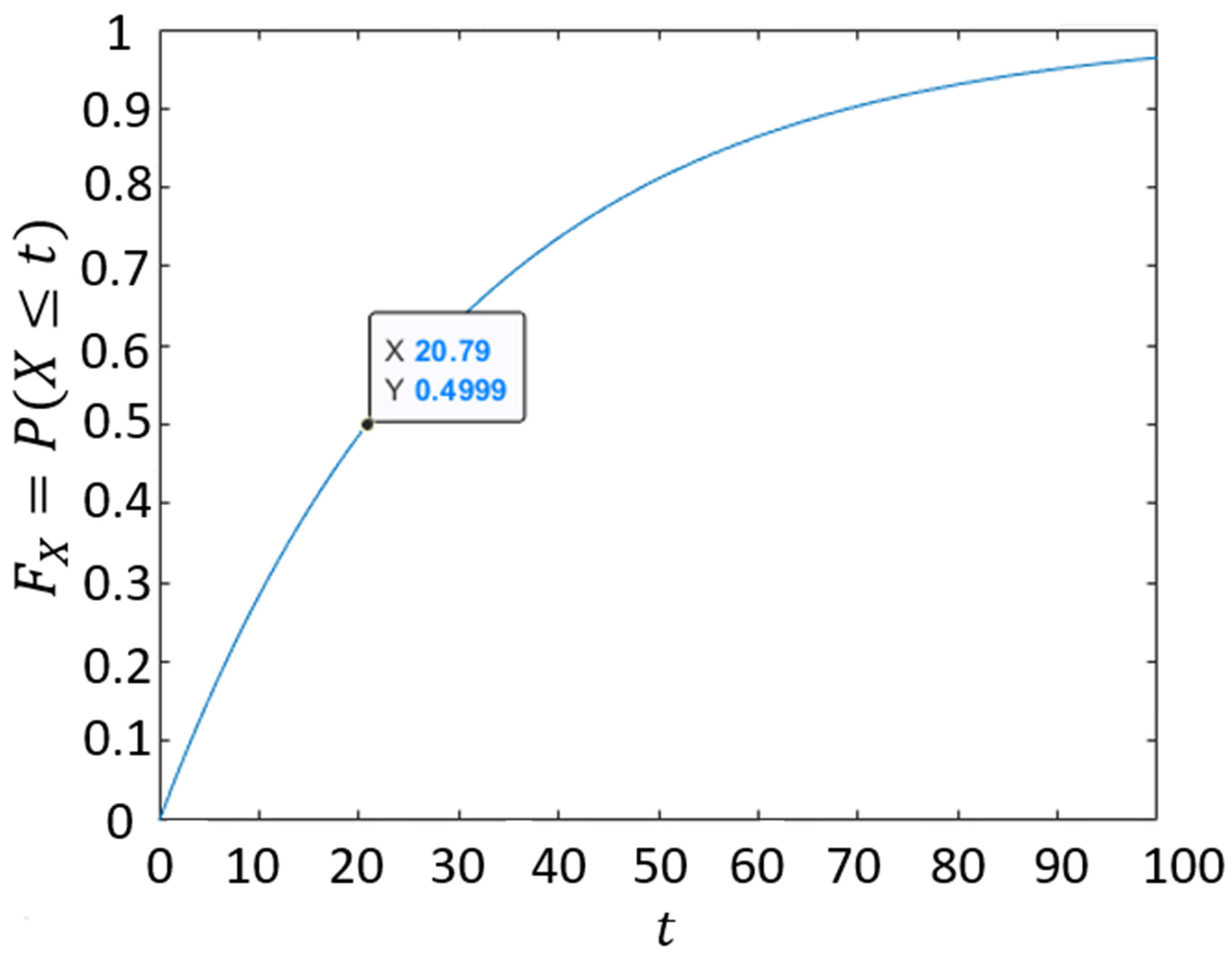
| The cumulative distribution function of the attacker′s time-to-success in a game with index k. | |
| The number of defender “take” moves between time and t; in other words, the first “take” move that is counted by is the “take” move at time ; thus, the “take” moves at times and are not counted in . | |
| The time since the last defender “take” move in a PLADD game with index , assuming the last defender “take” move before time t occurred either at time 0 or at time . | |
| The probability that the attacker controls a PLADD game with index k at time t. Note that if t is at an exact time where a defender “take” move occurs (i.e., instantaneously), we define as equal to . | |
| The probability that the attacker controls the parallel PLADD system at time t. | |
| EPS | Expected probability of success. It is computed as shown below: |
| -periodic | A -periodic function is a function with period equal to . |
| Testcases | |||||||
|---|---|---|---|---|---|---|---|
| 1 | 0 | 0 | 90 | 90 | 30 | 30 | 0.5372 |
| 2 | 0 | 45 | 90 | 90 | 30 | 30 | 0.4194 |
| 3 | 30 | 45 | 90 | 90 | 30 | 30 | 0.4236 |
| Testcases | |||||||
|---|---|---|---|---|---|---|---|
| 1 | 0 | 0 | 90 | 90 | 30 | 30 | 0.8348 |
| 2 | 0 | 45 | 90 | 90 | 30 | 30 | 0.8991 |
| 3 | 30 | 45 | 90 | 90 | 30 | 30 | 0.8494 |
| Testcases | ||||||||||
|---|---|---|---|---|---|---|---|---|---|---|
| 1 | 0 | 0 | 0 | 90 | 90 | 90 | 30 | 30 | 30 | 0.62909 |
| 2 | 0 | 0 | 45 | 90 | 90 | 90 | 30 | 30 | 30 | 0.52004 |
| 3 | 0 | 45 | 0 | 90 | 90 | 90 | 30 | 30 | 30 | 0.63435 |
| 4 | 0 | 45 | 45 | 90 | 90 | 90 | 30 | 30 | 30 | 0.58903 |
| Testcases | ||||||||||
|---|---|---|---|---|---|---|---|---|---|---|
| 1 | 0 | 0 | 0 | 90 | 90 | 90 | 30 | 30 | 30 | 0.77963 |
| 2 | 0 | 0 | 45 | 90 | 90 | 90 | 30 | 30 | 30 | 0.84917 |
| 3 | 0 | 45 | 0 | 90 | 90 | 90 | 30 | 30 | 30 | 0.75229 |
| 4 | 0 | 45 | 45 | 90 | 90 | 90 | 30 | 30 | 30 | 0.75229 |
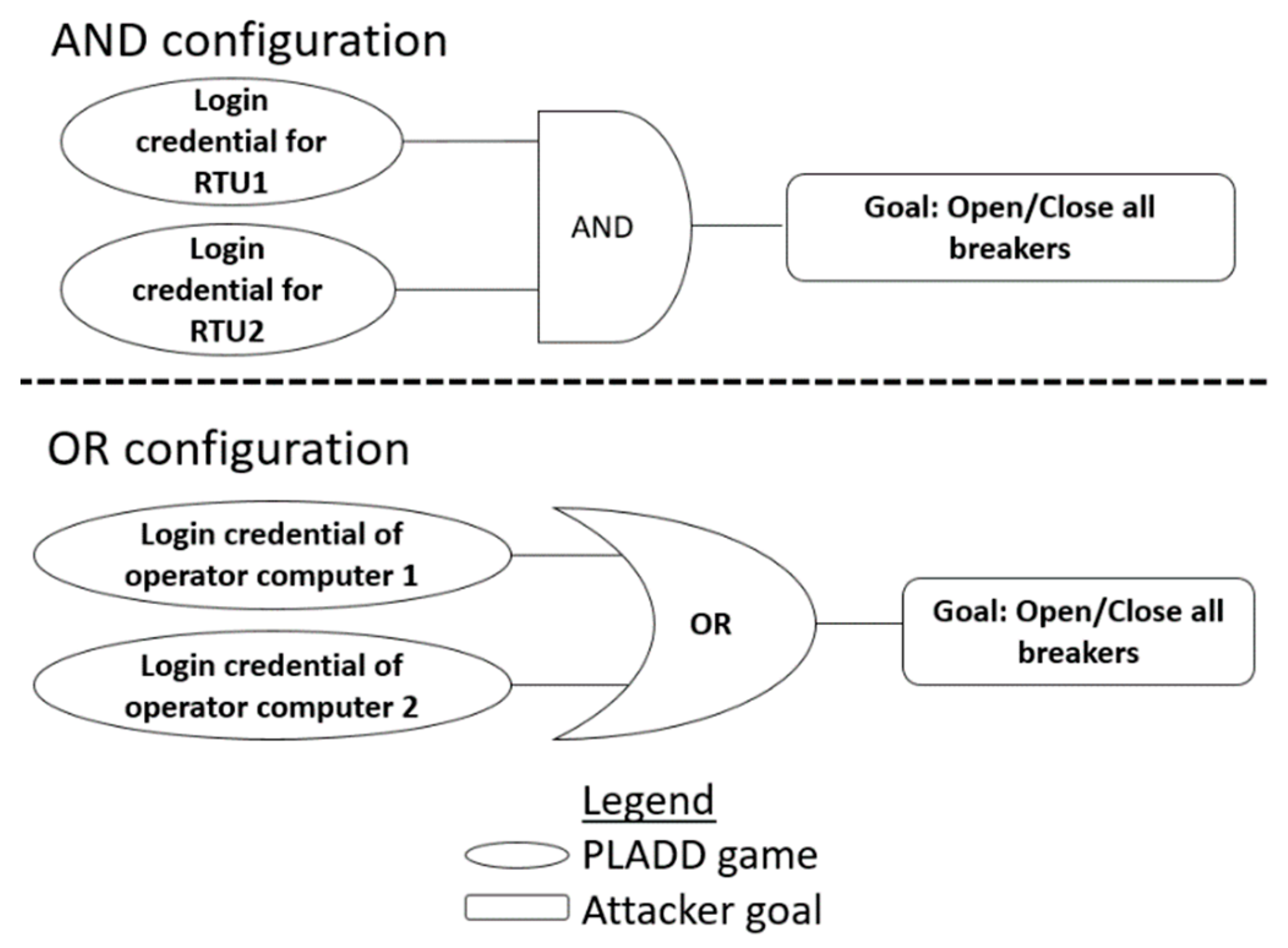
| Figure 6 AND configuration | Simulation # | Player Parameters (Days) | PLADD Game Offsets (Days) | EPS | Percent Improvement |
| 1.a | dRTU1 = 0, dRTU2 = 0 | 0.169 | |||
| 1.b | dRTU1 = 0, dRTU2 = 30 | 0.121 | 33.1 | ||
| 1.c | dRTU1 = 0, dRTU2 = 45 | 0.113 | |||
| 1.d | dRTU1 = 0, dRTU2 = 60 | 0.117 | |||
| 2.a | dRTU1 = 0, dRTU2 = 0 | 0.059 | |||
| 2.b | dRTU1 = 0, dRTU2 = 30 | 0.040 | 37.3 | ||
| 2.c | dRTU1 = 0, dRTU2 = 45 | 0.037 | |||
| 2.d | dRTU1 = 0, dRTU2 = 60 | 0.038 | |||
| 3.a | dRTU1 = 0, dRTU2 = 0 | 0.379 | |||
| 3.b | dRTU1 = 0, dRTU2 = 60 | 0.281 | 30.6 | ||
| 3.c | dRTU1 = 0, dRTU2 = 90 | 0.263 | |||
| 3.d | dRTU1 = 0, dRTU2 = 120 | 0.270 | |||
| Figure 6 OR configuration | 1.a | dcomputer1 = 0, dcomputer2 = 0 | 0.567 | ||
| 1.b | dcomputer1 = 0, dcomputer2 = 30 | 0.585 | 3.57 | ||
| 1.c | dcomputer1 = 0, dcomputer2 = 45 | 0.588 | |||
| 1.d | dcomputer1 = 0, dcomputer2 = 60 | 0.586 | |||
| 2.a | dcomputer1 = 0, dcomputer2 = 0 | 0.3672 | |||
| 2.b | dcomputer1 = 0, dcomputer2 = 30 | 0.3673 | 0.08 | ||
| 2.c | dcomputer1 = 0, dcomputer2 = 45 | 0.3675 | |||
| 2.d | dcomputer1 = 0, dcomputer2 = 60 | 0.3674 | |||
| 3.a | dcomputer1 = 0, dcomputer2 = 0 | 0.749 | |||
| 3.b | dcomputer1 = 0, dcomputer2 = 60 | 0.766 | 3.10 | ||
| 3.c | dcomputer1 = 0, dcomputer2 = 90 | 0.773 | |||
| 3.d | dcomputer1 = 0, dcomputer2 = 120 | 0.772 |
| Simulation | Subsystem 1 | Subsystem 2 | ||||
|---|---|---|---|---|---|---|
| 1 | 0 | 0 | 0 | 0 | 0.696 | 0.751 |
| 2 | 0 | 0 | 45 | 45 | 0.814 | 0.695 |
| 3 | 0 | 22.5 | 45 | 67.5 | 0.743 | 0.806 |
| 4 | 0 | 22.5 | 0 | 0 | 0.687 | 0.761 |
| 5 | 0 | 45 | 0 | 0 | 0.712 | 0.781 |
| 6 | 0 | 45 | 0 | 45 | 0.656 | 0.852 |
| 7 | 0 | 45 | 9 | 54 | 0.688 | 0.844 |
| 8 | 0 | 45 | 22.5 | 0 | 0.679 | 0.834 |
| 9 | 0 | 45 | 45 | 0 | 0.656 | 0.852 |
| 10 | 0 | 45 | 45 | 22.5 | 0.699 | 0.823 |
| 11 | 0 | 45 | 45 | 45 | 0.712 | 0.781 |
Publisher’s Note: MDPI stays neutral with regard to jurisdictional claims in published maps and institutional affiliations. |
© 2021 by the authors. Licensee MDPI, Basel, Switzerland. This article is an open access article distributed under the terms and conditions of the Creative Commons Attribution (CC BY) license (https://creativecommons.org/licenses/by/4.0/).
Share and Cite
Chen, Y.-C.; Mooney, V.J., III; Grijalva, S. Grid Cyber-Security Strategy in an Attacker-Defender Model. Cryptography 2021, 5, 12. https://doi.org/10.3390/cryptography5020012
Chen Y-C, Mooney VJ III, Grijalva S. Grid Cyber-Security Strategy in an Attacker-Defender Model. Cryptography. 2021; 5(2):12. https://doi.org/10.3390/cryptography5020012
Chicago/Turabian StyleChen, Yu-Cheng, Vincent John Mooney, III, and Santiago Grijalva. 2021. "Grid Cyber-Security Strategy in an Attacker-Defender Model" Cryptography 5, no. 2: 12. https://doi.org/10.3390/cryptography5020012
APA StyleChen, Y.-C., Mooney, V. J., III, & Grijalva, S. (2021). Grid Cyber-Security Strategy in an Attacker-Defender Model. Cryptography, 5(2), 12. https://doi.org/10.3390/cryptography5020012