1. Introduction
In “When the Map Is Better Than the Territory”, Erik Hoel provides a formal theory of how a system can give rise to causal descriptions at multiple levels of analysis [
1]. The proposal has its origins in the formal definition of the measure
for consciousness in the Integrated Information Theory of Consciousness [
2]. The question of how to describe the causal relations of a system at different scales is closely related to the debates in mental causation in philosophy, where the focus has been on whether mental states (thoughts, beliefs, desires, etc.) can be causes of behavior in their own right, distinct from the physical quantities (neurons, brain chemistry, etc.) that realize the mental states. Of course, multi-scale causal analyses are not restricted to the relation between the brain and the mind. Similar concerns arise in micro- vs. macro-economic theory, or quite generally in understanding how the life sciences relate to the fundamental natural sciences. In many domains there is an accepted level of analysis at which the causal processes are described, while it is understood that these macro-causal quantities supervene on more fine-grained micro-level causal connections. Hoel provides a precise formal account of this supervenience and explains under what circumstances macro-causal descriptions of a system can emerge. By integrating causal concepts with information theoretic ones, Hoel argues that a macro-causal account of a system emerges from micro-causal connections when the coarser, more abstract causal description (the map) is more informative (in a sense that he makes formally precise) than the micro-causal relations (the territory).
Hoel’s account is one of the very few attempts to provide an explicit formalism of causal emergence, which one could apply to a (model of a) real system. While we will be critical of some of the core features of the account, we highly commend Hoel for developing this theory in precise terms. Unlike many other attempts to explain multi-scale causal descriptions, this theory is precise enough for us to pinpoint where we disagree. Our disagreements are not flaws or errors in the account that would refute the theory, but highlight consequences of the theory that we think violate important desiderata of what an account of causal emergence should satisfy. Specifically, our examples show that Hoel’s theory permits so-called “ambiguous manipulations” with rather significant ambiguity (
Section 3), and that the operations of abstraction and marginalization do not commute in his theory (
Section 4). The latter is a particularly unusual feature for a theory that aims to describe a system at multiple scales of analysis.
Like many formal accounts, Hoel is silent on the metaphysical commitments of his theory. That is, it remains open whether the causal emergence he identifies has an independent objective reality, carving nature at its joints, or whether it is merely a convenient way for an investigator to model the system. None of our concerns hinge on this issue and so we will similarly remain agnostic with respect to the metaphysical commitments. However, depending on the view one takes, the implications of our formal results are different: To the extent that one reads Hoel’s account as a description of objective reality, our results show that the description is not objective, but contains significant modeling artifacts. If instead one interprets Hoel’s account as merely epistemic, then the results point to an arbitrariness in the investigator’s model that is not well justified and that has misleading consequences.
We start by describing Hoel’s theory in
Section 2. We have adapted Hoel’s notation to improve clarity. Where we use different notation, we note the mapping to Hoel’s notation in the footnotes. We then provide our main counter-intuitive examples in
Section 3 and
Section 4 and discuss the implications of our examples for the desiderata of a theory of causal emergence. In
Section 5, we cover a few of further curiosities of Hoel’s account before closing in
Section 6.
2. Hoel’s Theory of Causal Emergence
Similar to other theories of emergence (see, for example, Shalizi and Moore [
3]), Hoel describes his theory in terms of a discrete state space
with a finite number of states
that characterize the micro-level states of the system under investigation. Micro states are connected to one another by state transitions that are fully specified in a transition probability matrix
, whose entry
specifies the probability
of the system being in state
at time
given that it was in state
at time
t. Given that there are no unobserved variables and all state transitions are from one time point to the subsequent one, the transition probabilities correspond to the interventional probabilities
that characterize the micro-level causal effect of the system at time
t on the system at time
. We thus have a simple model of the micro-causal relations.
There are various ways of interpreting this model. Hoel’s notation suggests an interpretation of the model in terms of a fully-observed one-step Markov process evolving over time with one variable that has n states. However, Hoel’s model makes no commitments about further features that a time series may or may not exhibit, such as stationarity. So, one can also read the transition probability matrix as simply specifying an input–output relation of a mechanism (where the input and output have the same state space). For those more familiar with causal Bayes nets, one could also just think of two variables X and Y (with the same state spaces) and use to specify the transition probability matrix. However, no marginal distribution is specified.
To simplify subsequent notation, we let the state transition probability matrix
specify the transition probabilities from states
of input variable
X to states
of output variable
Y, with the understanding that the state spaces of
X and
Y are identical.
1Now, given a micro-causal system described by the finite state space and a transition probability matrix , under what circumstances does a macro-level causal description with state space and macro-level transition probability matrix emerge?
Every coarser description of the system has to combine states of
into a smaller set of macro states
. While any partition that is a coarsening of
is in a trivial sense a macro-level description of the original system, Hoel’s theory aims at identifying particular coarsenings that amount to, what he calls,
causal emergence. These are coarsenings of the original state space with distinguishing features that make them intuitively more appropriate as (macro-)causal descriptions in their own right. Hoel maintains that
effective information is the relevant measure to identify macro-causal descriptions. Effective information has a variety of appealing characteristics that permit a connection between causal and information theoretic concepts. In particular, it specifies the average divergence that a specific intervention on the system achieves, compared to a reference distribution of interventions. The underlying idea is that effective information tracks in a precise sense how causally informative the current state of the system is for its future state. As with many information theoretic notions, effective information is defined not only in terms of the transition probabilities, but also in terms of the input distribution for the “sender”, i.e., in this case, the cause. While Hoel does not discuss his choice of input distribution extensively, we believe that the selection of a maximum entropy intervention distribution
over the state space of the cause is motivated by a desire to (a) uniquely determine the value of the measure, and (b) to use a distribution that explores the full causal efficacy of the cause without being affected by its states’ observed or marginal probabilities. Given the finite discrete state space
, the maximum entropy intervention distribution is just the uniform intervention distribution over the set of micro states:
Intervening with this distribution on
X results in the effect distribution
over
Y:
In other words,
simply computes the uniform average over all rows in the transition probability matrix. To see the effect of each specific intervention
, we want to compare
with
, the specific row of the transition probability matrix. Hoel uses the Kullback–Leibler divergence to compare how different these two distributions are. The
effective information (
) of a (micro-level) system
then takes the average of these divergences:
where
is the Kullback–Leibler divergence. As the form of Equation (
5) already indicates,
is the mutual information between the uniform intervention distribution
over the cause and the resulting effect distribution
:
One way of thinking about effective information is that it provides a measure of how distinct the causal effects of
X are on
Y, using the maximum entropy distribution as a reference distribution. Consequently, when we now consider a macro-level description
of
, where the state space
of
U is a coarsening
of the state space of
X (recall that the effect always has the same state space as the cause here), then combining states with similar transition probabilities can lead to an improvement of how distinct the causal effects of the remaining aggregated states are, i.e., the mutual information between cause and effect can be increased by abstracting to a macro-level description.
However, in order to fully determine the effective information of a coarsening of the micro space
, one has to specify what it means to intervene on a non-trivial macro state
u. That is, one has to specify what
is when
, for two distinct micro states
and
. Without much explanation or motivation, Hoel defines the intervention on a macro state to correspond to a uniform average of interventions on the micro states that map to the macro state: By slightly overloading notation, let
u stand both for a macro state and for the set of micro states
that correspond to it (similarly for
v and
in the effect). Then the intervention on macro state
u is given by:
In words: The intervention on macro state
u results in a probability of macro state
v that is given by intervening on all micro states
that correspond to macro state
u, averaging the resulting distributions over
Y uniformly, and then summing over those micro states
that correspond to macro state
v.
2With this definition in hand, the effective information of any coarsening of the micro state space
of the system
can be determined. According to Hoel then,
causal emergence occurs when a macro state space
that is a strict coarsening of the micro state space
maximizes effective information. That is, the brute force
3 version of the abstraction operation from micro to macro level is that one searches over all possible coarsenings of the micro space. The coarsened state space applies to both
U and
V. For each such coarsening
, one determines the effective information of
by considering a uniform intervention distribution over
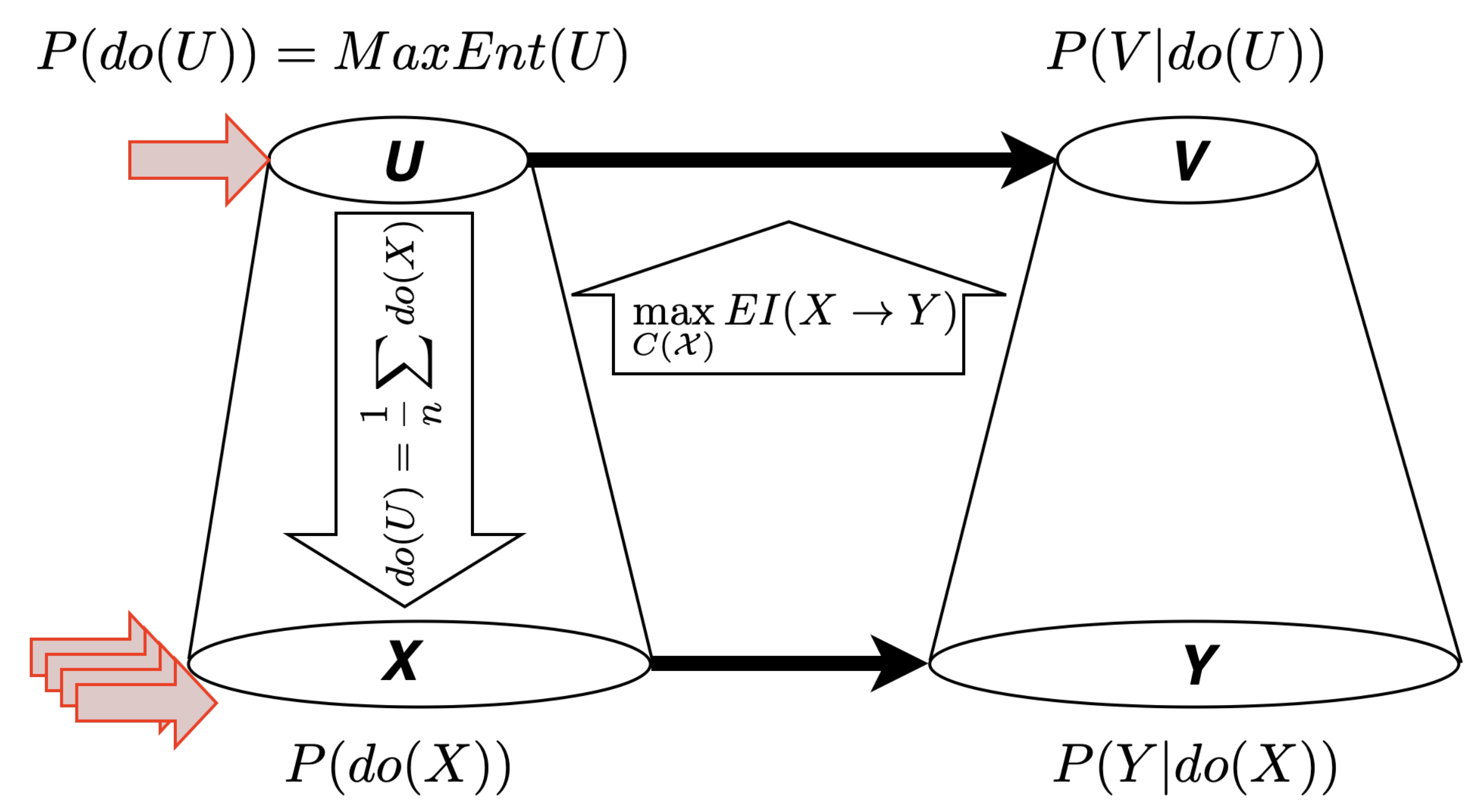
, the coarsened state space. This uniform intervention distribution over the coarsened state space will in general map to a non-uniform distribution over the micro state space (since the intervention probability on one macro state is divided up evenly among all the micro states that map to it, and different macro states may have different numbers of such micro states). There will be at least one partition that maximizes effective information. Whenever such a partition is coarser than the micro-level partition, Hoel speaks of
causal emergence. See
Figure 1.
This approach has many attractive features. In particular, it builds a close connection between macro-causal descriptions and channel capacity in information theory. Channel capacity is defined in terms of the input distribution that maximizes the mutual information between sender and receiver across a noisy channel:
Hoel’s search for causal emergence is similar: It is a search over intervention distributions over the
micro states in
for the intervention distribution that maximizes the mutual information between the intervened macro cause
U and the resulting effect
V. However, as the differing notation already suggests, the maximization of effective information is a maximization of mutual information subject to two constraints: First, only a subset of possible distributions over
X is considered—namely those that correspond to maximum entropy distributions (i.e., uniform distributions in this case) over some coarsening
of the micro space
. And second, rather than just maximizing mutual information between the sender and receiver, the maximization of effective information requires identical state spaces for the cause and effect.
4Hoel refers to the maximization of effective information as achieving the
causal capacity:
5Thus, a macro-level causal description
emerges from a micro-level causal system
whenever the effective information matches the causal capacity. This is when the map is better than the territory.
Despite the suggestive connection to information theory, several aspects of the definitions give reason for pause: Maximum entropy distributions are theoretically useful distributions, but they are an artificial addition to the analysis of a natural system. It remains an empirical question of whether such distributions have any relevance to the actual system one is investigating. Moreover, averages can obscure significant discrepancies, and in Hoel’s account of causal emergence there are at least two averaging steps: A macro-intervention is a uniform(!) average over the micro interventions that map to it, and effective information is a maximum entropy mixture (so, here again, a uniform average) over a set of KL divergences. Our examples in the following highlight what features of the territory are obscured by a map that uses maximum entropy and averaging of this kind.
3. Ambiguity: Merging States with Different Causal Effects
When two different micro states have the same transition probabilities, it is generally uncontroversial that they should (or at least, can) be combined to form a coarser macro state. The micro states do the same thing, so there is little point in distinguishing them. Indeed, effective information generally
6 does just that, as is illustrated by Hoel’s first example of causal emergence where he considers a micro state space with
possible states and a transition probability matrix given by
The first seven states have identical effects, so the EI is only 0.55. Unsurprisingly, the EI is maximized when the first seven states are collapsed, such that the macro state space
consists only of two states and the corresponding
is given by
This two-state macro representation has effective information of 1. More interestingly, as Hoel points out with his second example, the micro states need not have identical transition probabilities in order for a causal macro description to emerge. The following transition probability matrix over 8 states has effective information of 0.81, but collapsing the first seven states as above still maximizes effective information at 1.
Obviously, combining states 1–7 into a single state aggregates micro states with quite different causal effects. For example, state
has zero causal effect on states
and
, while state
loads 1/7 and 2/7 of its probability on states
and
, respectively. Defining macro variables, whose micro-level instantiations have different causal effects, results in macro variables that have so-called
ambiguous manipulations [
5]. Spirtes and Scheines illustrate ambiguous manipulations with the toy example of the effect of
total cholesterol on
heart disease. If
total cholesterol is constituted of high-density lipids (HDL) and low-density lipids (LDP), and HDL and LDL have different (say, for the sake of argument, opposing) effects on heart disease, then an intervention on
total cholesterol is
ambiguous, because its effect on
heart disease depends on the ratio of HDL to LDL in the intervention on
total cholesterol. Unless HDL and LDL have the quantitatively identical effect on
heart disease,
total cholesterol appears to be an over-aggregated variable. Indeed, there is reason to think that it was this sort of ambiguity that historically led to a revision of
total cholesterol as a relevant causal factor of heart disease. Instead, the causal relation was re-described in terms of its components, namely, HDL and LDL. The effect of
total cholesterol is just a mixture of two distinct finer-grained causal effects.
On Hoel’s account, the proportion of each of the micro state interventions is fixed by the uniform distribution over micro interventions described in (
8), which ensures a well-defined intervention effect, despite it being a mixture of different causal effects. It is as if an intervention on
total cholesterol always corresponded to a 50/50 intervention on HDL and LDL. Defining the macro intervention as the average over the micro interventions is, of course, possible, but entirely ad hoc. Why does an intervention on a macro state correspond to many different, presumably simultaneous, interventions on the corresponding micro states? Moreover, why should these micro-state interventions all be weighted equally? For example, when we set a thermostat to
F (macro state), then Hoel’s theory claims that the resulting effect is the uniform average over all ways that one could have set the gas particles’ kinetic energies such that their mean is
F. This includes micro states with highly uneven distributions over the kinetic energies of the particles, which can have causal consequences that are very different from those we typically associate with
F. It seems more realistic to instantiate such a macro intervention in terms of one specific micro state that corresponds to
F at the macro level—for example, it could be the micro state corresponding to
F that is closest to the actual state of the system at the time of intervention. Moreover, Hoel’s definition implies that one may have to average over completely contradictory micro-level effects: If we have two micro states that map to the same macro state, but one has the effect that the animal in a cage remains alive, whereas the other has the effect that it is killed, then the intervention on the macro state implies that the animal is half-dead, not that it is either dead or alive.
There are various ways one might respond. Some of the responses depend on whether one thinks of Hoel’s theory as describing what is actually happening in a given system or whether one thinks of it as a model of the investigator’s knowledge of the particular system. In the latter case the average over possible micro interventions can be construed as a strategy to handling the epistemic uncertainty about which micro state it might be that instantiated the macro intervention. We will not pursue these routes given that Hoel does not indicate whether the theory should be understood epistemically or metaphysically, but they are discussed in greater detail in Dewhurst [
6]. We only note that if one indeed views Hoel’s account as a model of the epistemic state of the investigator, then the investigator might deserve some freedom of thought: Maybe they prefer distributions other than the uniform one over the micro interventions because they have domain knowledge. Maybe they would update their distributions as more evidence comes in? Maybe they are aware of the critiques of objective Bayesianism and its use of uninformative priors. If one allowed for any such epistemic freedom, then the entire story would need to change because there would not be one causally emergent system, but a whole set of admissible macro descriptions.
One can try to avoid philosophical debates, by holding out hope that such dramatic cases as the above examples suggest, do not arise in the first place: If indeed the transition probabilities of the micro states are very different from one another (such as states 1–7 vs. state 8 above), then they would not be collapsed into one macro state, because that may not maximize the effective information. Indeed, in extreme cases, this is true—after all, the remaining two states in the matrix in (
12) are kept distinct.
So, how different can the causal effects of two micro states be such that they still end up being collapsed on Hoel’s theory?
Of course, any answer to this question has to specify a distance metric between causal effects (represented here by the rows in the transition probability matrix) and then has to maximize the distance between the two causal effects while ensuring that maximizing effective information of the system still collapses them into the same macro state. Even for systems with three micro states, we are not aware of any analytical solution to this problem for any non-trivial distance-measure. Given a
transition matrix, there would be six unknowns:
Each possible macro description of the system leads to combining these unknowns in different ways to determine the macro transition probabilities. Setting the effective information of one of these macro descriptions to be the maximum determines which macro description is chosen. Due to the definition of effective information (and the chosen distance metric), this gives inequality constraints in which the involved fractions and logarithms have different arguments depending on how many micro states are being collapsed. Even for these simple systems, we only have numerical results.
Consider a micro-level state space with three states
and a transition probability matrix given by
The effective information for this matrix is
, but effective information is maximized when the first two states are collapsed, resulting in a macro state space
and a corresponding transition probability matrix
Its effective information is
, slightly higher than for the micro level. In this case, the absolute distance
between the two rows of the collapsed states
and
in the transition probability matrix is 0.8. The maximum difference one can achieve using this distance measure is slightly higher, since one can still adjust the transition probabilities by tweaking further digits after the decimal point. Moreover, this matrix is not unique in having an absolute distance of 0.8 between the causal effects of two states and yet collapsing them. In
Appendix A, we give additional examples. We also consider what happens when one uses other distance metrics, such as the standard Euclidean distance, the maximum difference between any single transition probability from one state, the maximum of the minimum difference between any transition probability from any state, or—if one instead thinks of these causal effects as distributions—one could use the KL divergence as distance metric.
We give examples for all these cases (and one could pursue many more), but the upshot is the same: The examples have two states with rather different transition probabilities that are collapsed according to Hoel’s account. In what sense can we speak in these cases of causal emergence? At what point are micro-causal effects so different that grouping them together as a macro-effect does not amount to describing the system causally at the macro level, but instead amounts to describing mixtures of lower-level effects? In the example in (
14) above an intervention on state
has a small chance in resulting in state
and a roughly even chance in resulting in state
or
. In contrast, an intervention on state
results with probability 0.7 in state
, and roughly equal small probability in state
and
. Given the distinct causal effects of states
and
, it makes the choice of collapsing them very counter-intuitive despite the information theoretic result. Yet, on Hoel’s account, which intervenes on all states with equal probability, these two states are grouped together and the example would constitute a case of the emergence of a macro-causal description.
Of course, there is no contradiction in Hoel’s claims, and indeed state
provides a starker contrast to both
and
than they do to each other. But note that if we changed the first row of the transition probability matrix in (
14) to
, i.e., shifting just
of probability from the
to
, then the transition probabilities of states
and
would still look more similar to each other than either does to those of
, and yet states
and
would not be collapsed by maximizing effective information. So, it is not as if the causal emergence as defined here tracks any sort of intuitive clustering of close states. Maximizing effective information results in a very specific mixture of states and it remains quite unclear why the resulting clustering is privileged over any other intermediate (or additional) clustering.
The goal, we think, of identifying causally emergent macro descriptions is that we do not just have mixtures of underlying causal effects, but that the identified macro variable can be described as a cause in its own right, and that its micro instantiations are distinguished by differences that are in some sense negligible or irrelevant. This requirement will come as no surprise to those familiar with the literature on mental causation in philosophy, since it is closely related to the demand that macro causes be
proportional to their effect (see, e.g., Yablo [
7]). Although Yablo uses somewhat different terminology, a
proportional cause is the coarsest description of the cause that screens off any finer-grained description of the cause from the effect. That is, it is the coarsest description of the cause for which all interventions are unambiguous.
However, from the formal perspective the absence of ambiguous interventions is a more delicate desideratum. We expect that few would disagree that maximally coarsening while maintaining unambiguity indeed results in a macro-level model with all the features one would expect of a causal model. But the concern is whether the requirement is too strong: If one can only have macro states with unambiguous manipulations, then, for example, the system described by the transition probability matrix in Hoel’s second example (see (
13)) could not be coarsened at all.
There are two responses to this: First, indeed the perfect lack of ambiguity is too demanding, so one should permit the collapsing of states that have very similar causal effects, as defined by some distance metric between causal effects. This is exactly what is done for the identification of macro-causal effects in the Causal Feature Learning method of [
8,
9]. But second, beyond the slight distinctions in causal effect, one might want to bite the bullet on this concern: If the effect granularity is very fine, then indeed it seems appropriate that one should not coarsen the cause, since small changes in the cause may result in fine changes in the effect. But if the effect granularity is coarse, then automatically, it will be possible to also coarsen the cause while preserving unambiguity. For example, in order to predict where exactly the soccer ball will hit the goal, one might need the very precise description of the cause and, consequently, no coarsening (without violating ambiguity) is possible. But if one only wants to know whether the ball is going left or right (like a goalie during a penalty kick), then even a very coarse description of the cause can remain unambiguous.
This suggests a different modeling approach to Hoel’s: While Hoel described the system in terms of one state space that causally influences itself over time, the present considerations suggest that one should disentangle the coarsening of the cause from that of the effect. There can be cases where one can be coarsened while the other cannot. This is in contrast to Hoel’s case where the cause and effect always get coarsened together, because they are described by the same state space.
4. Commutativity: Abstraction and Marginalization
A macro description of a system is an abstraction of the underlying system [
10]. Hoel’s account focuses on coarsenings of the state space, but he explicitly notes at the beginning of his
Section 3 that such an abstraction can also occur over time and space [
1]: “Macro causal models are defined as a mapping
, which can be a mapping in space, time, or both”. The discrete time steps
, etc., used to define the Markov process are of arbitrary, but fixed, length. As in any time series, these are features of the model reflecting the rate of measurement. Of course, we would expect different causal processes to emerge if we consider longer or shorter time scales, just as we expect different causal descriptions for coarser or finer state spaces. But the marginalization of time steps and the abstraction over the state space should commute: Aggregating to coarser state spaces and then looking at the system at different time scales should result in the same macro-level description as looking at the system at different time scales, and then aggregating.
7 Similarly, if we view Hoel’s model only as specifying the input–output relations of a mechanism, then the concatenation of mechanisms (even of identical mechanisms) and abstraction should commute: Aggregating each mechanism by its own lights and then concatenating the aggregated mechanisms vs. concatenating the mechanisms and then aggregating the joint mechanism should result in the same macro-level description.
This is not the case for Hoel’s account: Let
denote the abstraction operation, i.e., the transition probability matrix of the corresponding macro state space
which maximizes the EI. If abstraction and marginalization commute, then the following equation has to be satisfied:
That is, finding the macro description of the effect over two time steps should be the same as evolving the macro description for two time steps.
Consider the following transition probability matrix for a micro state space
with three states:
The left hand side of Equation (
16) becomes
None of the states are collapsed, and the EI is
If we now consider the right hand side of Equation (
16), then
This resulting transition probability matrix collapses states 1 and 2 and has EI
. Not only does the EI not match, but the resulting systems have different state spaces depending on whether one marginalizes first and then abstracts, or abstracts first and then marginalizes.
Unlike in
Section 3, where we give specific transition probability matrices that maximize the distance between two states that get collapsed, this sort of failure of commutativity occurs in general for Hoel’s account. Only very specific transition probability matrices satisfy commutativity of abstraction and marginalization, most violate it. We note that in this case we have used a Markov process over the same variable
X with transition probabilities given in (
17). If one considered a causal system with three micro variables
X,
Y and
Z, each with their own state spaces, connected in a causal chain
, then marginalizing
Y could result in even more extreme discrepancies, because the transition probability matrices
and
would not have to be the same.
Thus, in Hoel’s account, whether causal emergence occurs at all and what the resulting macro description looks like depend on the order in which state space and time evolution are considered. Ultimately, this should not come as a surprise. Hoel’s account of causal emergence depends not only on the causal relations from one time step to another (which are described by the conditional distribution ), but also on the injection of the input distribution . Since Hoel’s input distribution has nothing to do with the system in question, but is an exogenous maximum entropy distribution, a discrepancy arises when one marginalizes time points whose marginal distribution does not correspond to the maximum entropy distribution naturally.
If abstraction and marginalization do not commute, then the macro-causal account does not actually describe features of the underlying system in question, but features that crucially depend on the rate of measurement (if we think in terms of time series) or on the input–output points (if we think of
as a mechanism) chosen by the investigator. A macro-level description of the system would be, so to speak, “bespoke” for the specific start and endpoint, but would not be generalizable or extendable. It would confirm the view of those who hold little regard for causal models in economics or psychology because (they think) their macro-level causes lack a degree of objectivity. This sort of reasoning quickly risks implying the impossibility of causal modeling quite generally in all but the most fundamental sciences. Consequently, for those who are more optimistic about causal models in the special and life sciences, it should come as no surprise that the demand for commutability of abstraction and marginalization is explicit in [
11] (in fact, their consistency demands are even stronger) and [
10]. The account of natural kinds in Jantzen [
12] pursues a somewhat different goal, but the core feature of the natural kinds is also the commutability of intervention and evolution of a system.
Even if one does not require that abstraction and marginalization commute at all time points, at the very least, they should commute at some suitably large intervals to ensure that the macro level description does not completely diverge from the micro level one. Given the sensitivity of Hoel’s account to the intervention distributions, even “occasional commutativity” (however one might reasonably define that) is generally not possible.
5. Further Comments
One of the attractive features of Hoel’s account of causal emergence is the integration of causal with information theoretic concepts. We noted in
Section 2 the theoretical similarities between Hoel’s causal capacity and the information theoretic channel capacity. Indeed, Hoel shows with several examples that as the number of possible micro states increases, that the causal capacity
can approximate the channel capacity, because the uniform intervention distribution at the macro level generally results in a “warped” distribution over the micro states.
8 We are not aware of any formal characterization or proof of this convergence claim.
9 But even if we grant that suitably general conditions can be found to support the claim that reaching causal capacity closely corresponds to exploiting channel capacity, then this is still a peculiar macro description of a natural system: Channel capacity in information theory is a normative concept. It describes the input distribution the sender
ought to be using in order to optimize information transmission. But a sender who does not use the optimal input distribution obviously does not exploit the channel capacity. The situation applies analogously to causal capacity: If we describe the micro state space of a system and its transition probabilities, then we can determine the causal capacity analytically. If there is causal emergence, then there is a coarsening of the micro state space that maximizes effective information. But whether or not the system actually exploits that causal capacity is an empirical question: It may not employ a maximum entropy distribution over the coarsened state space to maximize its causal effectiveness, just like an inexperienced sender may not use the optimal distribution for the noisy channel they are communicating over. Hoel seems to recognize this concern in the following passage from his paper:
“Another possible objection to causal emergence is that it is not natural but rather enforced upon a system via an experimenter’s application of an intervention distribution, that is, from using macro-interventions. For formalization purposes, it is the experimenter who is the source of the intervention distribution, which reveals a causal structure that already exists. Additionally, nature itself
may intervene upon a system with statistical regularities, just like an intervention distribution. Some of these naturally occurring input distributions
may have a viable interpretation as a macroscale causal model (such as being equal to
at some particular macroscale). In this sense, some systems may function over their inputs and outputs at a microscale or macroscale, depending on their own causal capacity and the probability distribution of some natural source of driving input.” (emphasis added) [
1]
Thus, Hoel’s account is about
potential causal emergence of a system, but not about
actual causal emergence.
10 So, even if we otherwise accept the account as a correct formalization of causal emergence, it remains an empirical question of whether a system actually exhibits its potential causal emergence of the form Hoel describes or not. Just like channel capacity in information theory, causal capacity is a normative concept.
A second consideration is that while the maximum effective information (EI) of a system is always unique, it is far from clear whether the corresponding partition that maximizes EI is unique. That is, there may be multiple equally appropriate macro-level descriptions of the same system. Sometimes cases like this are inevitable given the definition of causal emergence: Given a partition with three states, one can generally make the transition probabilities of two states more and more similar such that at some point the two-state partition maximizes the EI. Along the way, there will be a point where the two-state and the three-state partition will both maximize EI. Such cases are expected as there has to be a transition point from micro-level description to causal emergence, and the two partitions with equal maximum EI are hierarchical (one is a coarsening of the other). However, we postulate that it is also possible that two different-sized partitions of the same micro space,
neither of which is a coarsening of the other, may both maximize EI. That is, we postulate that there exist state transition probabilities for, say, a 5 state micro system such that its 3 state coarsening, the partition
, and its 2-state coarsening, the partition
, both maximize EI. In this case, two macro descriptions emerge that both describe the system macroscopically, but in entirely different ways. If such cases indeed exist as we suggest
11, then one can, of course, still dismiss them as inevitable edge cases. However, with an increasing number of states, one may want to make sure that such cases are not common. Moreover, even if there is no exact equality in the maximized EI of two very different partitions, or if such cases are rare, a near-match would already appear to make the causal emergence highly unstable. It would be interesting to have examples of real cases where such “incommensurate” macro descriptions seem plausible or appropriate.
Finally, science studies systems at many different scales: Economic theory supervenes on the interactions of the individual economic agents, those agents’ behavior supervenes on the underlying biology, which in turn supervenes on chemical and physical processes. We describe the causal interactions of this system at all of these scales, and at several in between. Yet, causal emergence, as Hoel has defined it, picks out one scale beyond the microscopic one (and perhaps other closely related macro scales that happen to result in the same effective information; see previous point). But it does not explain causal descriptions at multiple (>2) significantly different scales: How should we think about these intermediate scales? Do they not constitute a form of causal emergence? Are there any restrictions of which meso-scale descriptions of a system actually describe genuine causal relations?
These questions interact with the concern about causal capacity mentioned before: Given that causal capacity is not optimal from an information theoretic point of view (but at best approximates channel capacity) and that the system may not actually be exploiting the causal capacity in the first place, then what distinguishes the particular coarsening that Hoel identifies? Why is such a coarsening then still privileged over all the other intermediate coarsenings, or even those that constitute an over-aggregation according to Hoel’s account?


