An Algorithm for Indoor SARS-CoV-2 Transmission

Abstract

We propose a computer modeling approach for SARS-CoV-2 transmission that can be preferable to a purely mathematical framework. It is illustrated its functionality in a specific case of indoor transmission. Based on literature, we assume that infection is due to aerosols with viral particles that persist and accumulate for hours in the air even after the persons who produced them left the space. We incorporate also restricted opening hours as a mitigation measure and one possible behavioral change in response to this measure. It is shown via several examples how this algorithmic modeling approach can be used to run various scenarios in order to predict the efficacy of the intervention.

Introduction

The SARS-CoV-2 pandemic prompted an enormous research interest from various fields [1,2]. There is an understandable rush to public dissemination due to the global impact of the pandemic and the urgency for effective measures [3,4]. Of particular importance is the work on creating and analyzing epidemiological models [5]. This is because, as imperfect as they are, models are the default tools in making predictions on the evolution of the epidemic and in drafting public policy. On the other hand, data on all features related to this epidemic is inherently scarce due to the novelty of the disease [6,7]. This will improve as time and experience accumulate but, in the meantime, we can still develop theoretical models that test for various plausible scenarios so they can be ready for testing as soon as relevant data emerge.

Many epidemic models are purely mathematical in nature. Even a cursory overview of Mathematical Epidemiology reveals that there is always a compromise between the complexity of the model and the ability to analyze it fully in the form of abstract theorems [8,9]. The more complex (and more realistic) the model is the harder it becomes to use purely mathematical tools and the more reliance on numerical methods and simulations. Furthermore, incorporating control measures in the model brings unique challenges. One may want to predict the effect of these measures and, with each variation, the mathematics may change sufficiently to warrant a new analysis. Instead, we argue that, in some situations, it may be better and more practical to start, from the beginning, with a computer-based model which is capable to contain features that are difficult to even formulate in mathematical equations let alone analyze them. This approach presents itself with several advantages such as: modularity (extra features can be added to the program as needed without the need to start from the beginning), speed of implementation and prediction of outcomes, possibility of running and testing competing scenarios for intervention in the epidemic. These can be implemented quickly in the program without the need to reformulate and analyze from scratch an entire new model.

The purpose of this article is to illustrate this computer-based modeling approach by focusing on a single aspect of the epidemic as described below. Namely, we will focus on a certain type of transmission and how it relates to a specific type of policy designed to slow the spread of the virus. Generally speaking, these two are:

• the ability of the viral particles to linger in the air for hours in closed spaces and to infect susceptible people even after the source (the infected person) left the space [10].
• the use of restriction on opening times for various locations such as stores, bars or other businesses in an attempt to reduce the contact time among people [11].

Discussion

Remark 1

We emphasize that our goal here is not to build a complete SARS-CoV-2 model. Rather, we provide a proof-of-concept algorithm that is focused on a narrow “slice” of very specific population dynamics and control measures assumptions. Therefore, our program is NOT to be used as a standalone tool for predicting the epidemic and the effect of control measures. In fact, such a tool will necessarily contain many more additional modules and there will be numerous variations adapted to a particular community.

Early in the pandemic, there was enough evidence to suggest that most of the transmission occurs indoor and a small number of infected people are responsible for a large number of new infections (the so-called super-spreader events) [12]. A potential key mechanism is that aerosols with viral particles linger more time in the air compared to other similar viruses. They can stay airborne for hours before settling down and therefore they can accumulate in small spaces where a relatively high number of individuals come and go. A brief description of the mechanism is provided by the United States Environmental Protection Agency (EPA) on their website https://www.epa.gov/coronavirus/indoor-air-and-coronavirus-covid-19. There are also many proposed mitigation measures against indoor transmission and other non-pharmaceutical interventions [13,14].

One important consequence of indoor transmission is the possibility that someone can be infected even if that person enters an empty store if that space was visited in the past couple of hours by someone infected. This risk gets higher the smaller the space is and the more people come in and out [15,16]. Furthermore, while people stay physically apart, they may, unknowingly, still transmit the aerosols from one another. Put it differently, if the virus lingers in the air for several hours, two people who visited the same spot within that time interval can be considered as being in physical contact for all practical purposes. Note that the effect of wearing masks can be included in the model by adjusting downward the transmission probability term depending on the multitude of factors such as: compliance, quality of masks, etc. [17,18].

At the same time, in some regions, there were restrictions on opening times for stores and other businesses as part of the measures taken to slow down the spread of the virus. These actions can be both voluntary or enforced by authorities [19,20]. Notice that just this single intervention method implies lots of different assumptions. First of all, the rationale behind this policy depends on the type of location. Non-essential places like bars and restaurants were closed to simply reduce the number of contacts. Essential businesses such as grocery stores had restricted opening hours for various reasons: reduced staff availability, allowing time for re-stocking and sanitizing the store, etc. Moreover, voluntary restricted hours may or may not completely overlap with the mandated ones [21,22].

On the other hand, the pandemic and the control measures changed people’s behavior in a profound way. In particular, restricted opening times have the potential to interfere with the daily patterns of individuals. For example, if a store is closed but a similar one is open then a person may visit the open one at the time when he/she usually wants to shop. This, among other things, may cause certain locations to have an influx of visitors not normally encountered at various times of the day which may cause overcrowding if such locations are small [23,24]. Again, this is one out of many other possibilities such as: adjusting the schedule to visit when the favorite store is open, consolidating shopping trips into fewer ones, shopping only during week-ends, etc.

It is obvious that a purely mathematical modeling approach would be challenging if one needs a model to run different scenarios to analyze the effect of this control measure. In order to show how a computer algorithm can be implemented as an alternative, we will focus on the following behavior change from the ones mentioned above: the visiting of an alternate location that is open. In particular, the program will consider the aspect of preference ranking of locations of a population: if the most preferred location is closed, an individual will go to an alternative in the decreasing order of preference. Then we will run simulations for various scenarios that take into account restricted opening hours. We emphasize, again, that the program and the examples that we present are strictly limited to the basic assumptions that we make on the population dynamics and the distribution of opening times. These assumptions are for illustrating purposes and do not cover the entire complexity of a real-life situation. In the following section we establish these assumptions about the population and the transmission features together with the general description of the algorithm.

Population dynamics, epidemiology assumptions and the general algorithm

We will construct a “single issue” type of model by neglecting other possible social adaptations to the opening time restrictions such as: changing the time to visit when the favorite location is open, going on a different day, etc. Each of these can have its own implementation as part of a larger program. Furthermore, the overall dynamics is simplified as much as possible while still focusing on the key aspect of movement to various locations that are open. In what follows we will describe the population and its patterns.

Population dynamics assumptions

Suppose a population in a town is subject to a lock-down whereby only a fixed number of similar locations are open at various times (such as grocery stores). The underlying assumption is that, even if a pandemic wave justifies a lock-down, it may be necessary to still allow individuals to go out and obtain the essentials such as food and medicine [25,26]. We assume the following:

➢

At all times there is at least one location open.

➢

The population is split into groups by preference ranking of locations. That means, for each group there is a list of locations in decreasing order of preference. If a given location is closed, individuals in that group will consider going to the next location in that list if open and so on.

➢

Each individual, in a given hour of the day, is either at home or at one of these locations.

➢

Each individual represents his/her family unit (thus, if one individual is infected, we consider the entire family infected).

➢

Families rarely visit each other (this means infections at home will be rare).

➢

The rate of moving from home to an open location depends on the time of day (consistent with the window of time when a typical individual has the time to visit a store, for example). The rate of returning home from an open location depends on the typical time spent for that type of location (such as the average shopping time).

The epidemiology assumptions

Since the population is in a lock-down we consider that infection can only happen when visiting one of the open locations that are unavoidable to visit (again, for simplicity, we can think of them as grocery stores). We also assume that infection actually happens from inhaling the contaminated air produced by the infected from the present and the recent past. Thus, we have the following concepts:

➢

The viral load. Each location will have a current viral load and maximum viral load. The current viral load represents a measure of viral particles lingering in the air at a given moment of time which is proportional to the number of infected people who are inside that location at the present moment and up to several hours earlier (to account for the fact that the virus lingers in the air even after an infected person left the location). The maximum viral load represents the largest possible viral concentration in the air such that any additional infected person will not raise the infection risk in the air any further (in other words, the air is saturated as far as viral concentration is concerned).

➢

The infection mechanism. A susceptible individual may become infected from the contact with the contaminated air inside a location at a maximum infection rate that can only happen if the air has a viral saturation level (i.e., it reached its maximum possible viral load). Thus, the infection term is implemented according to the following formula:

$$\mathit{maximum}\_\mathit{infection}\_\mathit{rate}\times {\displaystyle \frac{\mathit{current}\_\mathit{viral}\_\mathit{load}}{\mathit{maximum}\_\mathit{viral}\_\mathit{load}}}$$

If the current viral load is less than the maximum viral load at that location, or:

maximum_infection_rate

If the current viral load reaches its maximum possible for that location.

The overall steps of the algorithm

The program will read the data from a file (described in the Appendix below) that contains the information about the population split by preference ranking groups, the open/close policies in a given day and the maximum infection rate. The program iterates by the current time value. The main steps are as follows:

➢

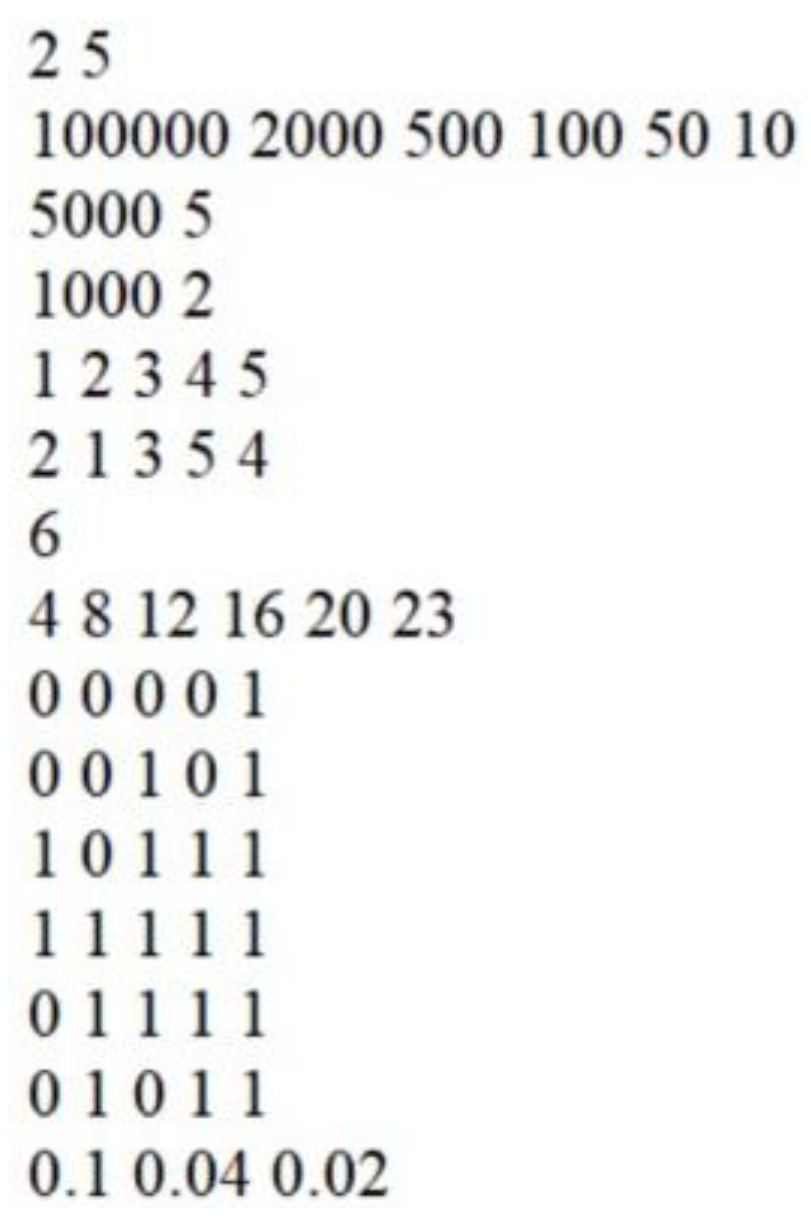
Step 1. Reading data from the input file. Initialize current time counter with 0.

➢

Step 2. Transfer from susceptible to infected at each location to account for new infections. Transfer from infected to recovered.

➢

Step 3. Transfer between home and open locations according to the preference ranking.

➢

Step 4. Transfer from recovered to removed to account for death from disease.

➢

Step 5. Writing the current size of susceptible and infected in the output file.

➢

Step 6. Increment current time value by 1.

➢

Step 7. If maximum running time is not reached go back to Step 2.

A more detailed pseudocode implementation of the algorithm, the format for the input data and several examples are provided in the Appendix. The examples were chosen to illustrate how this type of modeling approach can be used to assess whether an intervention moves the epidemiological situation in the right direction (i.e., fewer infections).

Remark 2

We can see from the examples that a certain open/closed configuration of locations may or may not cause fewer infections depending on whether susceptible individuals face these situations:

• they prefer to visit a large location with a large maximum viral load that is not easily reached,
• they find the most preferred location closed some or most of the time,
• their next choice in the preference ranking that is open happens to be a smaller location with a low maximum viral load that is easy to reach,
• they prefer to go to an alternative location rather than changing the shopping time,
• there is low or high masking quality and compliance.

Remark 3

The same type of analysis and simulation can be used to change the open/closed policy to avoid overcrowding the smaller spaces. It will require, first, surveying the population preferences and restrictions on movements followed by running simulations with various open/closed policies to narrow down those that actually slow the transmission.

Conclusions

We proposed a computer-based modeling approach for SARS-CoV-2 transmission that allows for fast adaptation to a multitude of assumptions and intervention scenarios which would otherwise be difficult to analyze strictly with mathematical tools. For demonstration purposes, we limited ourselves to an infection mechanism that is entirely based on the accumulation of aerosols in closed spaces. We incorporated in this program the mitigation measures based on opening or closing some locations at various times and the moving patterns among these locations by taking into account only the situation whereby an alternative exists for a closed location.

As mentioned from the beginning, our algorithm is designed as a proof of concept since it only takes into consideration a very narrow set of assumptions. As such, neither the model herein nor the accompanying examples can be used as stand-alone tools for describing the epidemic. It only shows how one can go from a set of assumptions to an algorithm ready for analyzing various scenarios. Its main advantage is that it can be easily extended toward more realism without the need for restating and proving new theorems as is the case in a purely mathematical model. Even within the narrow confines we set for our model it still has several limitations. For example, it assumes at least one location open at any given time. Thus, our model only considers the effect of opening policies on the choice of location to visit. In other words, we assume that there is always a location open that an individual is still willing to visit. The program does not take into account the effect of having all locations closed. This will require a dynamical modification of the transfer rates among locations since people are forced to adapt and find different shopping times. This, in fact will likely require a more in-depth survey of individual preferences and restrictions because finding a different time to shop than the typical one may need to take into account the working hours or other blackout times in a typical daily schedule. For better accuracy, it may be necessary to organize the input data by the individual rather than groups of a certain preference ranking. Another limitation is the use of the same transfer rates among locations for every day when, in reality, these will have to be further refined to account for whether certain people prefer certain days in the week to visit a location. We plan to work on these avenues in the near future.

Appendix

The pseudocode implementation of the algorithm. In this section we introduce the notations of all relevant variables and parameters, the implementation in pseudocode of the algorithm and several examples which were run using the programming language C++.

Notations and definitions

We denote by L the number of locations that can be visited when open. Each individual, at the current time n measured in hours, is either at home (identified as location 0) or at one of these away from home locations (labeled 1,2, · · · , L). From one hour to another, a certain fraction of the population moves from home to the most desired location that is open at that time in decreasing order of preference. At the same time, a proportion of individuals at each of the “away from home” locations will move back home. The rate of moving back home is denoted by a(n) and from home to the open location is b(n).

A preference ranking is the ranking of locations in decreasing order of preference for a group of people. Given L the number of locations and P the number of preferences we define the following: S[i][j][n] is the number of susceptible of preference i, at location j at time n, I[i][j][n] is the number of infected of preference i, at location j at time n and R[n] is the number of removed individuals at time n (this class combines the recovered or hospitalized, where i = 1, 2, · · · , P; j = 0, 1, · · · , L and n = 1, 2, · · · .

The maximum viral load for each location from 0 to L is denoted by N[0], N[1], · · · , N[L]. The current viral load for each location is denoted by N crt[0], N crt[1], · · · , N crt[L] and it is given by the number of infected people at each location up to 3 hours in the past (this number is an estimation and it may be different if experimental data shows a different value).

The λ is the maximum infection rate (when the location is at the maximum viral load). Therefore, the infection rate at a location j will be given by:

$$\lambda {\displaystyle \frac{Ncrt\left[j\right]}{N\left[j\right]}}\mathrm{if}Ncrt\left[j\right]<N\left[j\right]\mathrm{or}\lambda \mathrm{if}Ncrt\left[j\right]=N\left[j\right].$$

Each preference i from 1 to P is given by the row i of a matrix with P rows and L columns. Specifically, c[i][1], c[i][2],· · ·, c[i][L] is the ranking of locations in decreasing order of preference corresponding to preference i. For example, suppose we have 3 locations and:

c[2,1] = 3, c[2,2] = 1, c[2,3] = 2.

This means that for the group of people with the preference ranking number 2, their most preferred location is 3 followed by location 1 and finally by location 2. If 3 is closed and 1 is open they will choose to visit 1.

An opening policy is the open/closed information for each store in a given time interval within a day. The number of possible opening policies is not fixed and it is determined by how many times during a day the open/ closed status change. Let’s denote by T the number of opening policies. This means that the 24 hours duration of a day is split into T intervals starting with hour 0 and ending with hour 23 as follows:

0 < t[1] < t[2] < … <t[T] = 23.

For example if we have a certain policy for the time interval 0 to 7, another one for 7 to 20 and another one from 20 to 23 then T = 3, t[1] = 7, t[2] = 20, t[3] = 23. Each opening policy will be codified in a matrix with T rows and L columns. Specifically,

o[i][1], o[i][2], ⋯, o[i][L]

is the open/closed information for the opening policy i where the value of o[i][j] is either 1 if location j is open or 0 if location j is closed.

For example, suppose there are 3 stores and 2 opening policies as follows: t[1] = 15, t[2] = 23 and:

o[1,1] = 0, o[1,2] = 1, o[1,3] = 1

o[2,1] = 1, o[1,2] = 0, o[1,3] = 0

This means that, between the hours 0 to 15 the store 1 is closed but the stores 2 and 3 are open and between the hours 16 and 23 the store 1 is open and the other two are closed. The format for the input file is given in Figure 1.

The pseudocode of the algorithm can be accessed at https://github.com/s-gannon/Opening-Policy-Simulation

Let’s consider now several examples. Suppose we have a population where a significant portion prefers to visit a large store (see Figure 2). We can see that about 5000 of the total of 6000 susceptible prefers to visit store 1 which also has a large maximal viral load. The result of the simulation is shown in Figure 3. The susceptible class settles at 2000 after the epidemic is over which means that about 4000 were infected. We now change the input data file to restrict the open hours of the most preferred stores (thus forcing the population to visit the stores with lower maximal viral load) as seen in Figure 4. The result shown in Figure 5 shows that the susceptible settle now at about 1000 meaning that 5000 were infected by the end of the epidemic. This may suggest an unwanted effect, however, the maximum transmission rate λ = 0.2 remained the same. This may not be realistic if restricted opening times are accompanied by strict masking protocols which may have the effect of reducing the airborne viral particles. To take this into account, let’s consider the same input file but with a lower transmission rate λ = 0.1 (Figure 6).

The result shown in Figure 7 indicates that the susceptible settle at about 3000 leaving 3000 eventually infected. This, contrary to the previous case, indicates a positive effect of the measure.

Figure 1. Input data file format.

Figure 1. Input data file format.

Figure 2. Preferred locations open most of the time.

Figure 2. Preferred locations open most of the time.

Figure 3. Preferred locations open most of the time.

Figure 3. Preferred locations open most of the time.

Figure 4. Restrictions on the preferred locations.

Figure 4. Restrictions on the preferred locations.

Figure 5. Restrictions on the preferred locations.

Figure 5. Restrictions on the preferred locations.

Figure 6. Restriction on the preferred locations and masking protocols.

Figure 6. Restriction on the preferred locations and masking protocols.

Figure 7. Restriction on the preferred locations and masking protocols.

Figure 7. Restriction on the preferred locations and masking protocols.

Conflict of interest disclosure

There are no known conflicts of interest in the publication of this article. The manuscript was read and approved by all authors.

Compliance with ethical standards

Any aspect of the work covered in this manuscript has been conducted with the ethical approval of all relevant bodies and that such approvals are acknowledged within the manuscript.

References

1. Carraturo, F.; Del Giudice, C.; Morelli, M.; Cerullo, V.; Libralato, G.; Galdiero, E.; Guida, M. Persistence of SARS-CoV-2 in the environment and COVID-19 transmission risk from environmental matrices and surfaces. Environ Pollut. 2020, 265 Pt B, 115010. [Google Scholar] [CrossRef]
2. Al Huraimel, K.; Alhosani, M.; Kunhabdulla, S.; Stietiya, M.H. SARS-CoV-2 in the environment: Modes of transmission, early detection and potential role of pollutions. Sci Total Environ. 2020, 744, 140946. [Google Scholar] [CrossRef] [PubMed]
3. Fisman, D.N.; Tuite, A.R. Evaluation of the relative virulence of novel SARS-CoV-2 variants: a retrospective cohort study in Ontario, Canada. CMAJ. 2021, 193, E1619–E1625. [Google Scholar] [CrossRef]
4. Stroe, A.Z.; Stuparu, A.F.; Axelerad, S.D.; Axelerad, D.D.; Moraru, A. Neuropsychological symptoms related to the COVID-19 pandemic experienced by the general population and particularly by the healthcare personnel. J Mind Med Sci. 2021, 8, 197–208. [Google Scholar] [CrossRef]
5. Oude Munnink, B.B.; Worp, N.; Nieuwenhuijse, D.F.; Sikkema, R.S.; Haagmans, B.; Fouchier, R.A.M.; Koopmans, M. The next phase of SARS-CoV-2 surveillance: real-time molecular epidemiology. Nat Med. 2021, 27, 1518–1524. [Google Scholar] [CrossRef]
6. Giovanetti, M.; Benedetti, F.; Campisi, G.; Ciccozzi, A.; Fabris, S.; Ceccarelli, G.; Tambone, V.; Caruso, A.; Angeletti, S.; Zella, D.; Ciccozzi, M. Evolution patterns of SARS-CoV-2: Snapshot on its genome variants. Biochem Biophys Res Commun. 2021, 538, 88–91. [Google Scholar] [CrossRef]
7. Meo, S.A.; Meo, A.S.; Al-Jassir, F.F.; Klonoff, D.C. Omicron SARS-CoV-2 new variant: global prevalence and biological and clinical characteristics. Eur Rev Med Pharmacol Sci. 2021, 25, 8012–8018. [Google Scholar] [CrossRef]
8. Araújo, M.B.; Mestre, F.; Naimi, B. Ecological and epidemiological models are both useful for SARS-CoV-2. Nat Ecol Evol. 2020, 4, 1153–1154. [Google Scholar] [CrossRef]
9. Koelle, K.; Martin, M.A.; Antia, R.; Lopman, B.; Dean, N.E. The changing epidemiology of SARS-CoV-2. Science. 2022, 375, 1116–1121. [Google Scholar] [CrossRef]
10. Harrison, A.G.; Lin, T.; Wang, P. Mechanisms of SARS-CoV-2 Transmission and Pathogenesis. Trends Immunol. 2020, 41, 1100–1115. [Google Scholar] [CrossRef]
11. Lipsitch, M.; Krammer, F.; Regev-Yochay, G.; Lustig, Y.; Balicer, R.D. SARS-CoV-2 breakthrough infections in vaccinated individuals: measurement, causes and impact. Nat Rev Immunol. 2022, 22, 57–65. [Google Scholar] [CrossRef] [PubMed]
12. Zonta, F.; Scaiewicz, A.; Levitt, M. The Gompertz Growth of COVID-19 Outbreaks is Caused by Super-Spreaders. arXiv 2021, arXiv:2111.02962v2. [Google Scholar]
13. Bazant, M.Z.; Bush, J.W.M. A guideline to limit indoor airborne transmission of COVID19. Proceedings of the National Academy of Sciences 118, no. 17 (2021).
14. Mendez-Brito, A.; Bcheraoui, E.C.; Pozo-Martin, F. Systematic review of empirical studies comparing the effectiveness of non-pharmaceutical interventions against COVID-19. Journal of Infection 2021, 83, 281–293. [Google Scholar] [PubMed]
15. Azuma, K.; Yanagi, U.; Kagi, N.; Kim, H.; Ogata, M.; Hayashi, M. Environmental factors involved in SARS-CoV-2 transmission: effect and role of indoor environmental quality in the strategy for COVID-19 infection control. Environ Health Prev Med. 2020, 25, 66. [Google Scholar] [CrossRef]
16. Rencken, G.K.; Rutherford, E.K.; Ghanta, N.; Kongoletos, J.; Glicksman, L. Patterns of SARS-CoV-2 aerosol spread in typical classrooms. Build Environ. 2021, 204, 108167. [Google Scholar] [CrossRef]
17. Sima, R.M.; Olaru, O.G.; Cazaceanu, A.; Scheau, C.; Dimitriu, M.T.; Popescu, M.; Ples, L. Stress and anxiety among physicians and nurses in Romania during the COVID-19 pandemic. J Mind Med Sci. 2021, 8, 252–258. [Google Scholar] [CrossRef]
18. Hong, L.X.; Lin, A.; He, Z.B.; Zhao, H.H.; Zhang, J.G.; Zhang, C.; Ying, L.J.; Ge, Z.M.; Zhang, X.; Han, Q.Y.; Chen, Q.Y.; Ye, Y.H.; Zhu, J.S.; Chen, H.X.; Yan, W.H. Mask wearing in pre-symptomatic patients prevents SARS-CoV-2 transmission: An epidemiological analysis. Travel Med Infect Dis. 2020, 36, 101803. [Google Scholar] [CrossRef]
19. Shi, S.; Tanaka, S.; Ueno, R.; Gilmour, S.; Tanoue, Y.; Kawashima, T.; Nomura, S.; Eguchi, A.; Miyata, H.; Yoneoka, D. Travel restrictions and SARS-CoV-2 transmission: an effective distance approach to estimate impact. Bull World Health Organ. 2020, 98, 518–529. [Google Scholar] [CrossRef]
20. López, V.; Čukić, M. A dynamical model of SARS-CoV-2 based on people flow networks. Saf Sci. 2021, 134, 105034. [Google Scholar] [CrossRef]
21. Imborek, K.L.; Krasowski, M.D.; Natvig, P.; Merrill, A.E.; Diekema, D.J.; Ford, B.A. Experience With Pretravel Testing for SARS-CoV-2 at an Academic Medical Center. Acad Pathol. 2021, 8, 23742895211010247. [Google Scholar] [CrossRef]
22. Al-Saleh, M.M.; Alamri, A.M.; Alhefzi, A.A.; Assiri, K.K.; Moshebah, A.Y. Population healthy lifestyle changes in Abha city during COVID-19 lockdown, Saudi Arabia. J Family Med Prim Care. 2021, 10, 809–815. [Google Scholar] [CrossRef] [PubMed]
23. Salway, R.; Su, T.T.; Ismail, R.; Glynis Armstrong, M.E.; Foster, C.; Johnson, L. The impact of COVID-19 movement restrictions on physical activity in a low-income semi-rural population in Malaysia: A longitudinal study. J Glob Health. 2021, 11, 05029. [Google Scholar] [CrossRef] [PubMed]
24. Nicola, M.; Alsafi, Z.; Sohrabi, C.; Kerwan, A.; Al-Jabir, A.; Iosifidis, C.; Agha, M.; Agha, R. The socio-economic implications of the coronavirus pandemic (COVID-19): A review. Int J Surg. 2020, 78, 185–193. [Google Scholar] [CrossRef]
25. Yang, H.; Rao, Z. Structural biology of SARS-CoV-2 and implications for therapeutic development. Nat Rev Microbiol. 2021, 19, 685–700. [Google Scholar] [CrossRef]
26. Wilkin, P.J.; Al-Yozbaki, M.; George, A.; Gupta, G.K.; Wilson, CM. The Undiscovered Potential of Essential Oils for Treating SARS-CoV-2 (COVID-19). Curr Pharm Des. 2020, 26, 5261–5277. [Google Scholar] [CrossRef]