Article

Radiofrequency Bias Correction of Magnetization Prepared Rapid Gradient Echo MRI at 7.0 Tesla Using an External Reference in a Sequential Protocol

1
Department of Medical Radiation Physics, Clinical Sciences Lund, Lund University, 221 85 Lund, Sweden
2
Department of Linguistics and Phonetics, Lund University, 221 00 Lund, Sweden
3
Center for Medical Imaging and Physiology, Skåne University Hospital, 221 00 Lund, Sweden
*
Author to whom correspondence should be addressed.
Tomography 2021, 7(3), 434-451; https://doi.org/10.3390/tomography7030038
Submission received: 15 July 2021 / Revised: 27 August 2021 / Accepted: 9 September 2021 / Published: 13 September 2021

Abstract

:
At field strengths of 7 T and above, T1-weighted imaging of human brain suffers increasingly from radiofrequency (RF) B1 inhomogeneities. The well-known MP2RAGE (magnetization prepared two rapid acquisition gradient echoes) sequence provides a solution but may not be readily available for all MR systems. Here, we describe the implementation and evaluation of a sequential protocol to obtain normalized magnetization prepared rapid gradient echo (MPRAGE) images at 0.7, 0.8, or 0.9-mm isotropic spatial resolution. Optimization focused on the reference gradient-recalled echo (GRE) that was used for normalization of the MPRAGE. A good compromise between white-gray matter contrast and the signal-to-noise ratio (SNR) was reached at a flip angle of 3° and total scan time was reduced by increasing the reference voxel size by a factor of 8 relative to the MPRAGE resolution. The average intra-subject coefficient-of-variation (CV) in segmented white matter (WM) was 7.9 ± 3.3% after normalization, compared to 20 ± 8.4% before. The corresponding inter-subject average CV in WM was 7.6 ± 7.6% and 13 ± 7.8%. Maps of T1 derived from forward signal modelling showed no obvious bias after correction by a separately acquired flip angle map. To conclude, a non-interleaved acquisition for normalization of MPRAGE offers a simple alternative to MP2RAGE to obtain semi-quantitative purely T1-weighted images. These images can be converted to T1 maps, analogously to the established MP2RAGE approach. Scan time can be reduced by increasing the reference voxel size which has only a miniscule effect on image quality.

1. Introduction

The magnetization prepared rapid gradient echo (MPRAGE) sequence has become the standard for structural T1-weighted (T1-w) 3D imaging. The T1 contrast is obtained by an inversion pulse followed by a rapid gradient echo (RAGE) readout with optional delays for free recovery before and after the readout [1]. At ultra-high field (UHF) MRI (7 T or above), the signal-to-noise ratio (SNR) is improved through the increased polarization of nuclear spins, which can be translated into either increased spatial resolution or faster scan times. The former alternative allows for visualization of substructures, unfeasible at lower field strengths [2]. A major challenge of UHF is the increased inhomogeneity of the radiofrequency (RF) B1 field, which varies based on subject, positioning, and coil [3]. Because of the unpredictability of the B1 field, pixel values from images acquired at different scanning sessions are generally not reproducible. This means that an important requirement for longitudinal or multi-site studies is not fulfilled. The increased inhomogeneity applies to both the transmit (B1+) and the receive sensitivity components, which combine to form a total bias field, that diminishes the uniformity of the image. To correct for this intensity bias, it was suggested to acquire a reference gradient-recalled echo (GRE) in conjunction with the MPRAGE sequence [4]. Through a simple division of the two acquisitions, a normalized MPRAGE image is obtained where signal variations due to the shared receive coils are eliminated, thus improving image quality as well as reproducibility. B1+ affects the MPRAGE and the GRE pulse sequences differently through the local flip angle and, therefore, the related bias is reduced but not removed in the normalized MPRAGE. The division also removes the influence of proton density (PD) and T2*, thereby creating a purely T1-w image with improved tissue contrast. As the pixel values depend on the sequence, the technique is considered to be “semi-quantitative”. The reference GRE can be acquired either separately or interleaved with the MPRAGE at a longer inversion time (TI), and the latter approach has been popularized as the MP2RAGE (magnetization prepared two rapid acquisition gradient echoes) sequence [5].
In this work, we describe an implementation where MPRAGE and reference are acquired in a non-interleaved, sequential fashion to produce the normalized MPRAGE. This approach is an accessible alternative to the interleaved MP2RAGE which, initially, was not readily available on our 7T MR system. Although the non-interleaved variant is expected to be more susceptible to inter-scan subject motion, the reference GRE can be accelerated through enlarged acquisition voxels, allowing for shorter scan time. The optimization procedure focused on the reference GRE, specifically on the flip angle and voxel size, in an effort to improve contrast, SNR, residual B1+ bias, and scan time. The protocol was implemented at three different spatial resolutions, and normalized MPRAGE images acquired at a higher versus a lower spatial resolution were compared. The intra-subject and inter-subject reproducibility (crucial for a semi-quantitative protocol) were also investigated. Finally, the feasibility of calculating T1 maps from a look-up table (LUT) of the normalized signal, obtained by forward modelling, was explored. The latter approach extends beyond the semi-quantitative domain and results in fully quantitative maps which would allow for a more direct biophysical interpretation in terms of, for instance, myelination [6]. It is analogous to the approach described for the interleaved MP2RAGE by Marques et al. [5]. The work presented here documents an optimized protocol for bias field-corrected structural imaging at 7 T, easily implemented and interpretable by radiologists.

2. Materials and Methods

2.1. Theory

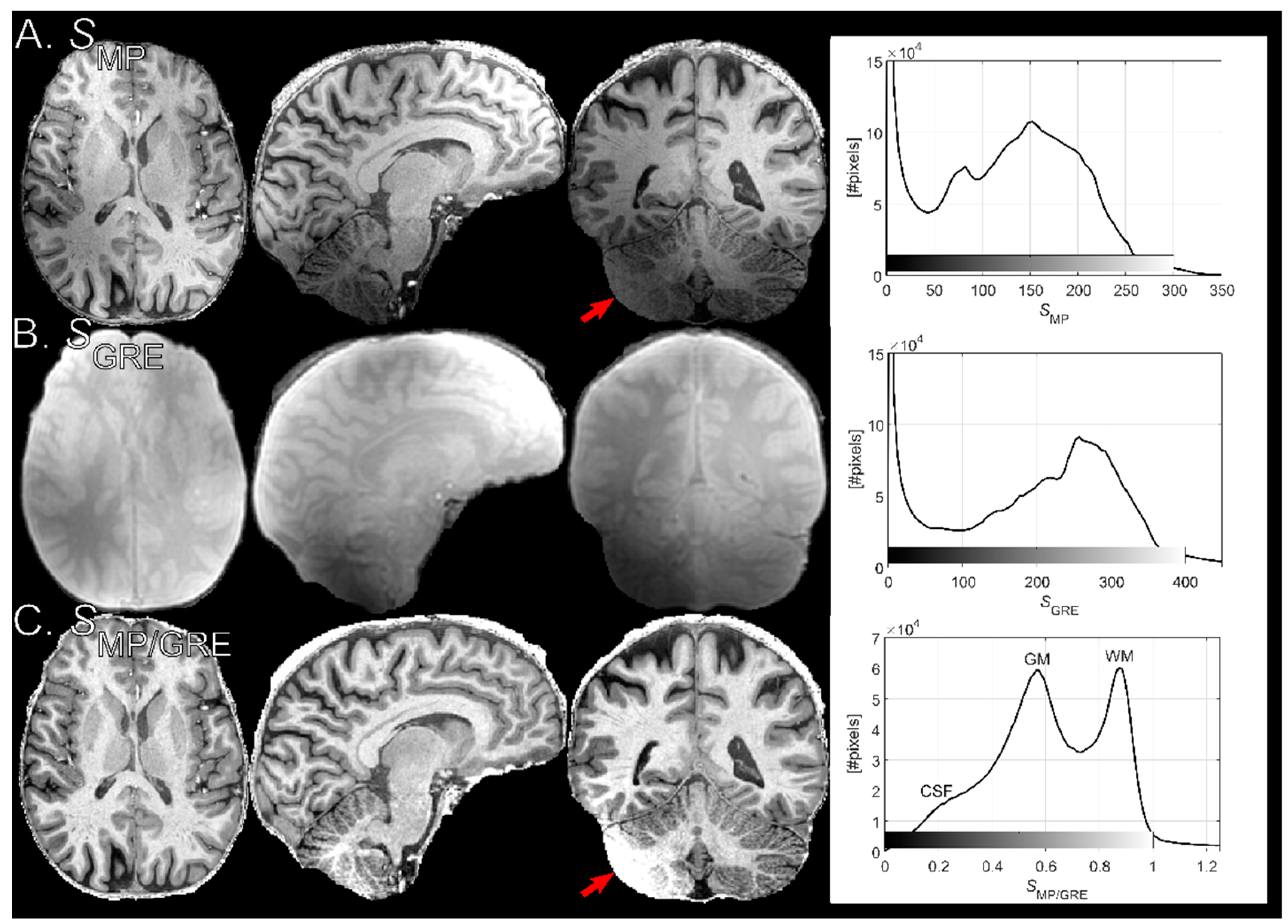
The influence of receive sensitivity, PD, and T2* were removed through division of the MPRAGE signal, SMP, by the reference GRE signal, SGRE, to yield the normalized MPRAGE signal, SMP/GRE. This rationale is illustrated by paraphrasing Equation (3) in [4]:
S MP / GRE = S MP S GRE f R ρ M ˜ z , MP sin ( f T α MP ) exp ( T E R 2 ) f R ρ M ˜ z , GRE sin ( f T α GRE ) exp ( T E R 2 ) = M ˜ z , MP sin ( f T α MP ) M ˜ z , GRE sin ( f T α GRE )
where ρ denotes PD, M ˜ z , MP , GRE = M z , MP , GRE / ρ is the longitudinal magnetization per unit PD, f R is a factor accounting for the spatial dependence of receive sensitivity (here, a weighted linear combination of individual channels). The arguments of the sine functions are the local flip angles, i.e., α loc , MP , GE = f T α MP , GE , where f T takes account of the transmit field (B1+) inhomogeneity. Finally, R 2 = 1 / T 2 is the effective transverse relaxation rate. Note that M ˜ z , MP is acquired under transient conditions towards a driven equilibrium, M ˜ 0 , with an increased rate R 1 = 1 / T 1 [7]:
M ˜ 0 = M ˜ 0 · 1 exp ( R 1 T R ) 1 exp ( R 1 T R )
where M ˜ 0 is the magnetization at thermal equilibrium ,   R 1 is
R 1 = R 1 ln ( cos ( f T α MP ) ) / T R ,
and R 1 = 1 / T 1 . If full relaxation within one cycle is not obtained, M ˜ z , MP will attain a dynamic steady-state between cycles, usually occurring after a few cycles [8]. The degree of agreement between M ˜ z , MP and M ˜ 0 when the central k-space line is acquired is a function of TI and T 1 as well as of the local flip angle and thus f T . Note that, without an inversion pulse, M ˜ z , GRE is always acquired under steady-state conditions so that
M ˜ z , GRE = M ˜ 0 ( f T α GRE , T 1 ) .
Thus, transmit field related bias may not be removed completely for α MP = α GRE as Equation (1) might imply.

2.2. Equipment

The protocols were implemented on an actively shielded 7T MR system (Achieva, Philips Healthcare, Best, The Netherlands), using a head coil with two transmitter channels and 32 receive channels (Nova Medical, Wilmington, MA, USA). Healthy subjects were scanned after giving informed written consent and the study was approved by the regional Ethical Review Board. Dielectric pads were used in the experiments [9].

2.3. MPRAGE Acquisition

The MPRAGE protocol was built upon the standard protocol for structural MRI available at the research site. Isotropic voxel sizes of either 0.73, 0.83, or 0.93 mm3 were acquired with a slab-selective excitation, a readout flip angle of αMP = 8°, TR = 8 ms, fat-water in-phase TE = 1.97 ms and a bandwidth/px of 503 Hz/px. For inversion, an adiabatic pulse with duration 22 ms and a maximal B1 amplitude of 15 μT was used. The delay from inversion to the central k-space readout (linear phase encoding) was TI = 1200 ms and the time between inversions was Tcycle = 3500 ms. These timings (i) allowed for a period of free relaxation after the readout train (increasing dynamic range) and (ii) ensured that the Mz of cerebrospinal fluid (CSF) was close to the zero-crossing during acquisition of the center of k-space. Both (i) and (ii) will improve T1 contrast in magnitude images. After each inversion, a single 2D plane of k-space was acquired so that the turbo factor (TF) was identical to the acquisition matrix size in the inner loop phase-encoded direction, Ny. Parallel imaging in the form of sensitivity encoding (SENSE) was applied in the outer loop (right–left direction) with a reduction factor of 2.5 [10]. The inner loop corresponded to the anterior-posterior (AP) direction. Switching between the different resolutions will alter TF and thus affect the T1 contrast (see Results 4.3). For (0.7 mm)3 resolution, a small inner loop SENSE reduction factor of 1.11 had to be applied to fit the readout train within TI = 1200 ms (TF = Ny/1.11). Note that the FOV in the outer loop (FOVFH,AP,RL = 230 × 230 × 180 mm3) can be enlarged without affecting contrast. SENSE-related wrap-around artifacts in the AP direction were avoided by an oversampling margin (default setting) which did not affect the acquisition time (Tacq). Lastly, to explore the possibility of further reducing Tacq, the protocol was implemented with elliptical k-space sampling in the phase encoding directions. A prerequisite for this kind of readout is a multi-shot acquisition combined with a zigzag k-space trajectory involving both phase encoding directions during the RAGE readout. This switching between the inner and outer phase encoding loops is performed in such a way that overall contrast is unaffected for constant TF. The acquisition matrix (Nx,y,z), TF and Tacq for all spatial resolutions with/without elliptical k-space phase encoding are listed in Table 1.

2.4. Reference GRE Acquisition

The steady-state GRE sequence was acquired with TR, TE, and outer loop SENSE factor identical to the MPRAGE sequence, but with 50% zero-filling in the outer loop to reduce scan time. In other words, voxel dimensions in the right–left direction were 1.4, 1.6, or 1.8 mm for the (0.7)3, (0.8)3, and (0.9)3 mm3 protocols, respectively. When determining the in-plane voxel size (see Results 3.2), the bandwidth/pixel was changed accordingly so that the absolute fat signal displacement was constant between GRE and MPRAGE. Receiver gain and flip angle were calibrated for MPRAGE and then kept constant during the GRE. After acquisition, the volume was reconstructed to the same matrix size as the MPRAGE through zero-filling.

2.5. Data Post-processing

Images in the Digital Imaging and Communications in Medicine (DICOM) file format were exported, pseudo-anonymized, and converted to the Neuroimaging Informatics Technology Initiative (NIfTI) file format using an in-house modification of the dcm2niix tool [11]. The platform-dependent scaling of signal intensities was reverted from stored values to 32-bit floating point/1000 (to obtain pixel values in the range of 0–1000) [12]. Spatial dimensions were re-ordered to transverse orientation according to radiological convention (right–left). Rigid co-registration of the reference GRE to the MPRAGE volume was performed using the FMRIB Linear Image Registration Tool (FLIRT) [13,14], where after the normalization was performed as in Equation (1). A mask of the brain was obtained by applying the Brain Extraction Tool (BET) to the PD-w reference GRE [15]. Segmentation of the three major tissue classes, white matter (WM), gray matter (GM) and CSF, was performed using the FMRIB Automated Segmentation Tool (FAST) [16]. Improvement in spatial homogeneity, after signal normalization, for different parameter settings of the reference GRE was analyzed using the coefficient-of-variation (CV) over the tissue classes in the normalized MPRAGE. The CV within a small WM ROI was used to evaluate relative changes in SNR; the rationale for this approach was that the CV in a spatially restricted ROI of homogenous tissue should be unaffected by B1+ and dominated by SNR. Average contrast between WM and GM was defined as C = S ¯ WM S ¯ GM S ¯ WM + S ¯ GM where S ¯ WM and S ¯ GM is the average pixel value of the respective segmented tissue type.

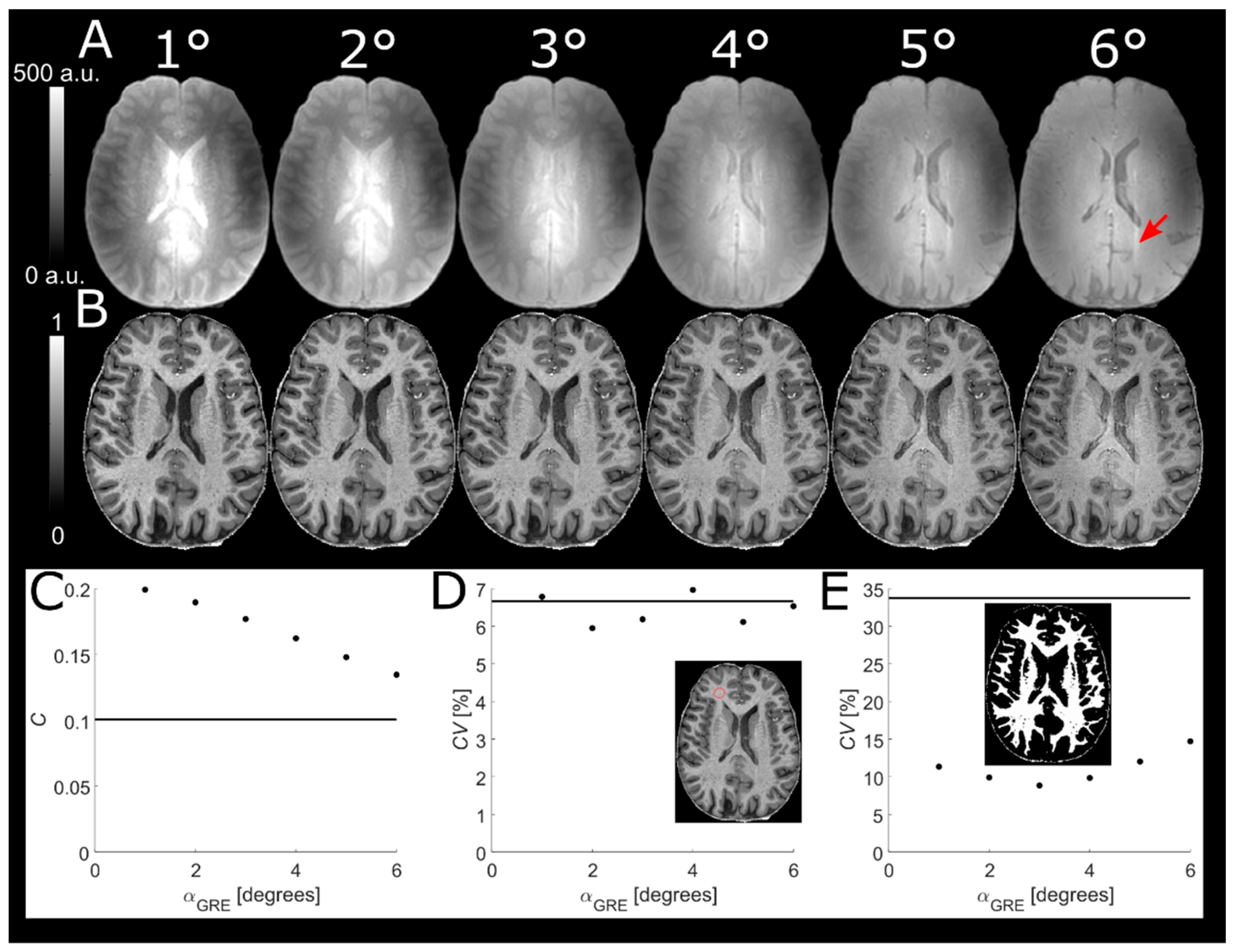
2.6. Readout Flip Angle of Reference GRE

A higher αGRE will increase the T1-w of the predominantly PD-w reference GRE, thus reducing tissue contrast in the normalized MPRAGE image. On the other hand, reducing αGRE below the Ernst angle will decrease SNR. To find a compromise between SNR and tissue contrast in the normalized MPRAGE, αGRE was varied from 1° to 6° in increments of 1° in a single subject. In order to obtain comparable pixel values, reference GREs were scaled by a global factor giving a scaled signal
S GRE , scaled ( α GRE , i ) = S GRE ( α GRE , i ) / ( α GRE , i 0.5 · α GRE , 6 2 + R 1 T R α GRE , 6 ( 0.5 α GRE , i 2 + R 1 T R ) ) ,
where a single R 1 = 0.83   s 1 (corresponding to expected WM T 1 1.2   s ) was used to approximate the saturation of Mz [17,18]. The scaling only served to facilitate identical windowing of the images and does not affect the analysis itself. The contrast between segmented WM and GM as well as the CV of segmented WM was plotted as a function of αGRE. The latter was used as a proxy to evaluate any residual influence of B1+ inhomogeneities.

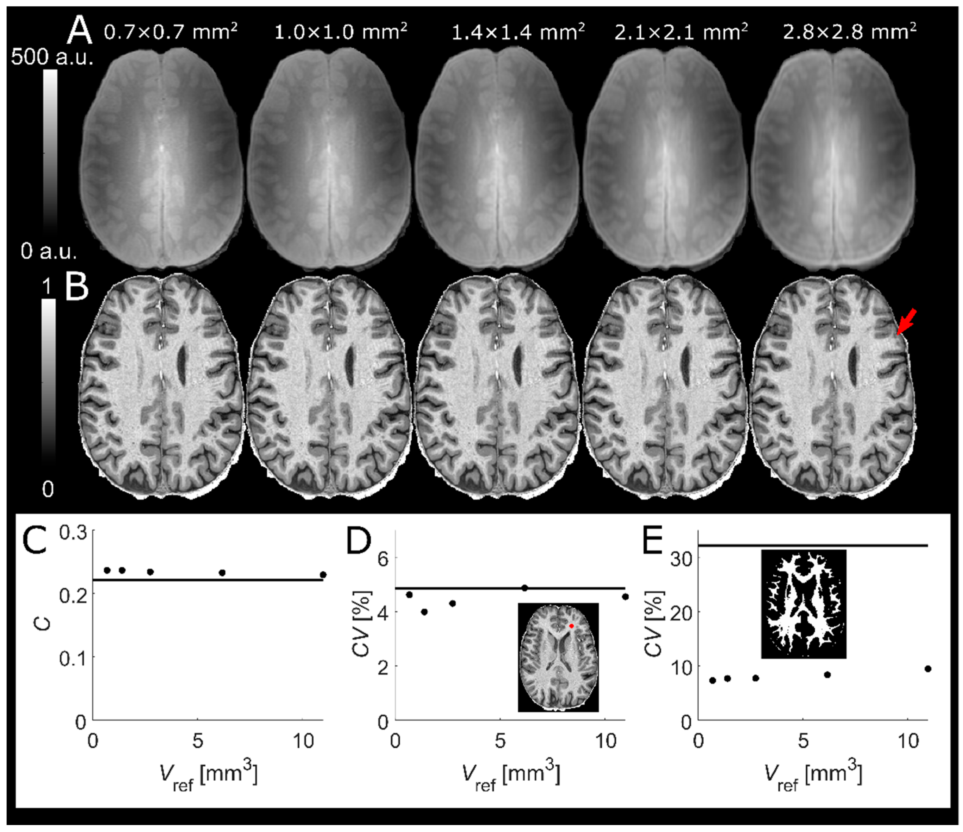
2.7. Voxel Size of Reference GRE

The B1-related intensity bias (of both receive and transmit effects) comprises mostly low spatial frequencies. Thus, a reference GRE with low spatial resolution is sufficient to correct for B1 inhomogeneity. On the other hand, this is not the case for PD and T2* contrast. If the normalized MPRAGE is purposed to produce only semi-quantitative images with a greatly reduced intensity field bias, some dilution of the “pure” T1 contrast could be acceptable to reduce scan time. In an effort to further reduce scan time and evaluate the effect on the resulting image quality, an MPRAGE volume with 0.7 mm isotropic resolution was normalized by a reference GRE for which the voxel size, Vref, was varied in-plane as 0.70 × 0.70, 1.05 × 1.05, 1.40 × 1.40, 2.10 × 2.10, and 2.80 × 2.80 mm2 (i.e., ×1, ×1.5, ×2, ×3, ×4 the MPRAGE resolution) in a single subject. The voxel dimension in the outer loop (right–left direction) was constant at 1.40 mm resulting in acquisition times of Tacq = 2:21, 1:35, 1:10, 0:49, and 0:37 min, respectively.

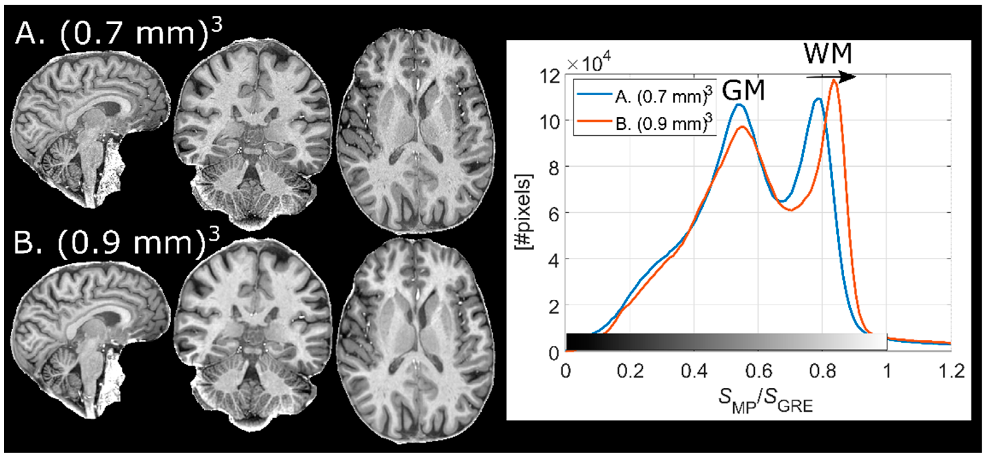
2.8. Implementation at Different Resolutions

Two finalized protocols (Results 3.1–3.2) with voxel sizes of (0.7 mm)3 and (0.9 mm)3 were used on a single subject to compare the effect of the corresponding TF on the contrast. Further, the potential increase of interpolation artifacts at different spatial resolutions (especially in the reference GRE) was of interest to assess.

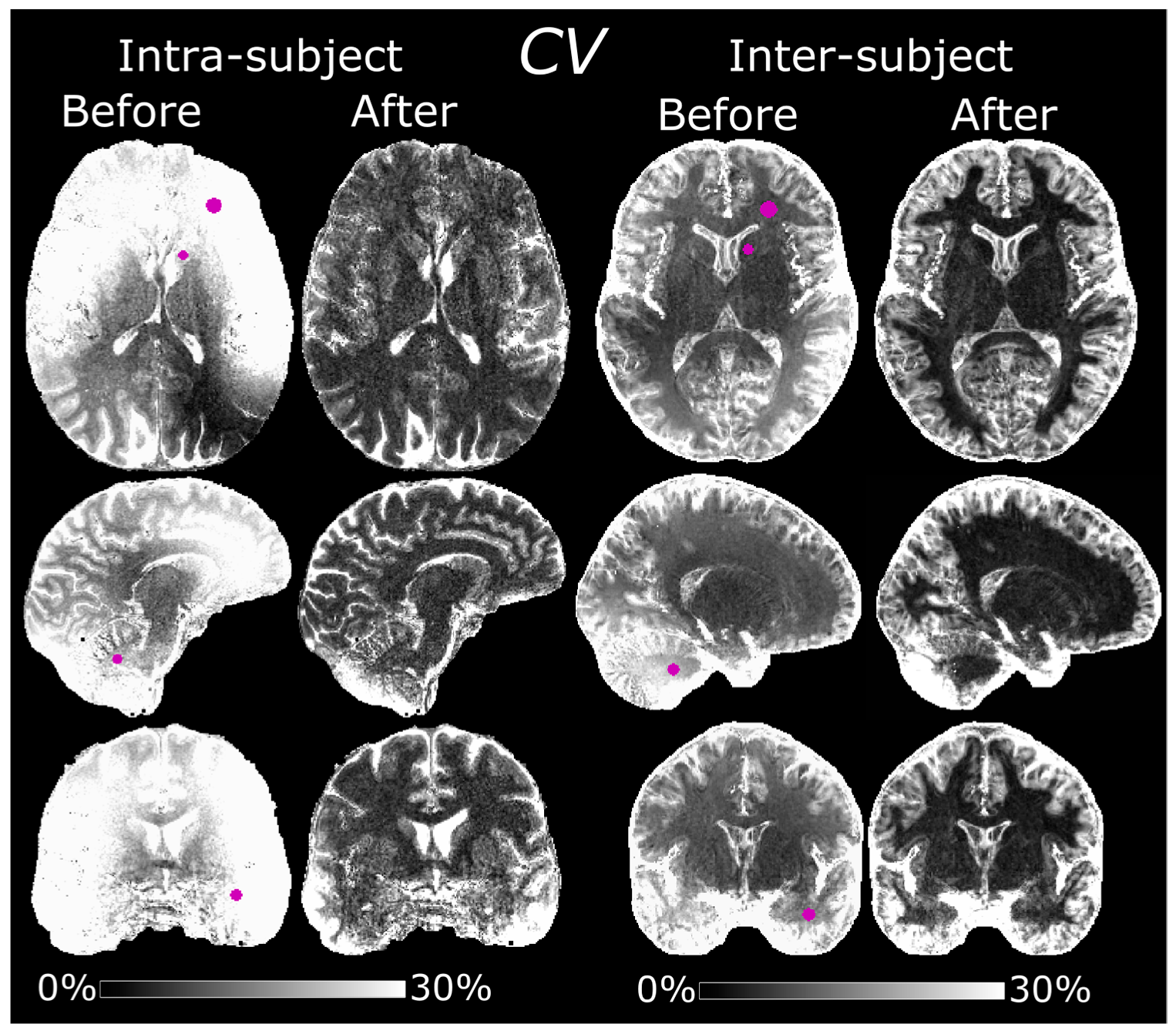
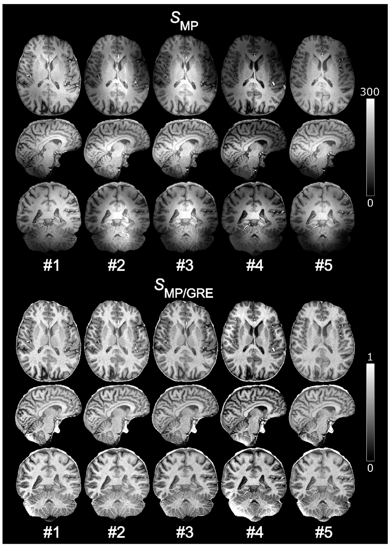
2.9. Intra-Subject Variability

One subject (male, 51 years old, body mass index (BMI) of 23.6) was scanned on five separate occasions over a period of about 8 months using the normalized MPRAGE protocol with 0.7 mm isotropic resolution. Maps of CV were compared before and after normalization and the average CVs in WM, GM, and CSF were calculated. Regions of interest (ROIs) were manually delineated in the CV maps to study local variability. The ROIs were defined in left frontal WM, the left caudate head, the cerebellum, and the left temporal lobe.

2.10. Inter-Subject Variability

The 0.8 mm isotropic resolution protocol was previously used in a separate work to study correlations between cortical morphology and language-learning aptitude [19]. From the underlying subject population of this work, a subset of 10 randomly chosen volunteers (7 female, 22 ± 1.9 years old) were used to examine the inter-subject variability of the normalized MPRAGE images. The subjects were all of normal build, that is, height, weight, and BMI were perceived to fall within the 5th and 95th percentiles. Images were diffeomorphically registered to the Montreal Neurological Institute (MNI) space using the diffeomorphic anatomical registration using exponentiated Lie algebra (DARTEL) algorithm as embedded in the statistical parameter mapping (SPM)-based histological MRI (hMRI) toolbox [20,21]. As in the previous subsection, maps of the CV were then compared before and after normalization and the average CVs in WM, GM, and CSF were calculated. ROIs were likewise defined in MNI space in the same four areas as in the previous subsection, i.e., left frontal WM, left caudate head, cerebellum, and the left temporal lobe. The average CVs in WM, GM and CSF were also calculated based on the average pixel intensities of individual segmentations rather than one common segmentation in MNI space.

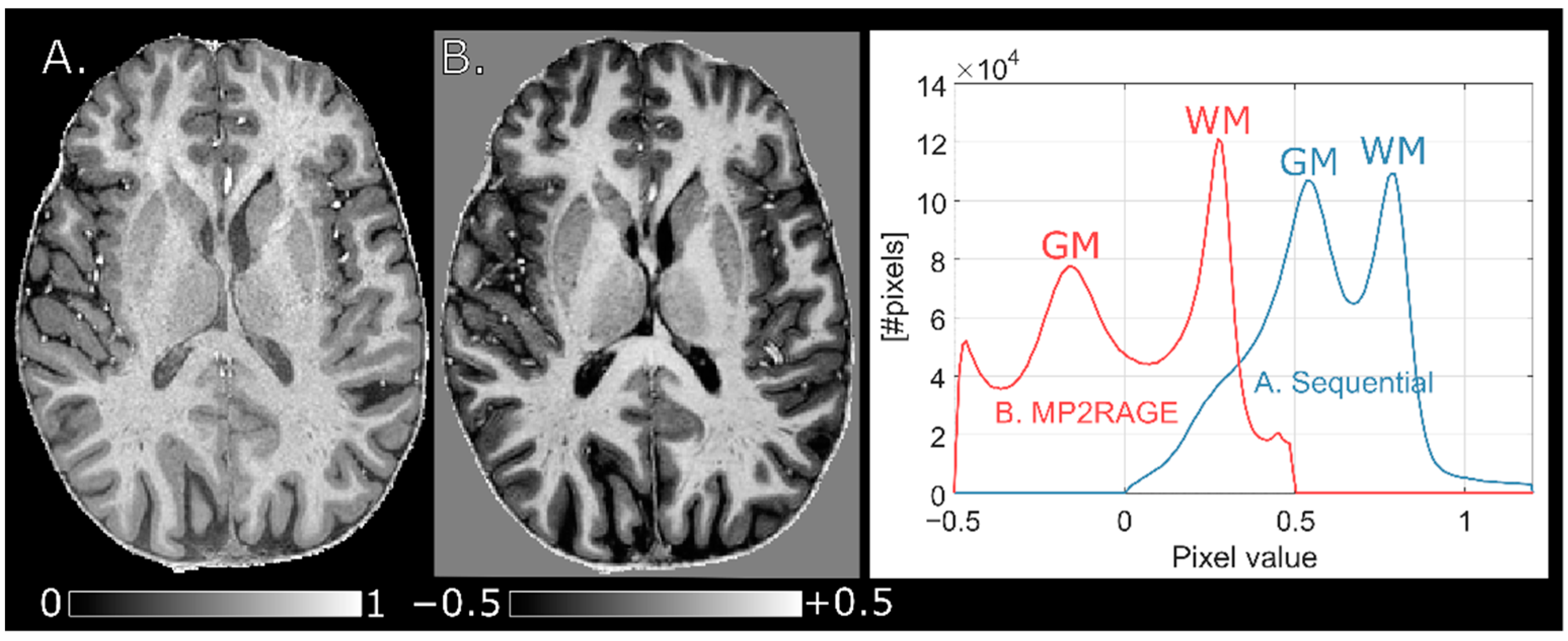
2.11. Comparison to MP2RAGE

The finalized (0.7 mm)3 sequential protocol was compared to an interleaved MP2RAGE protocol with the same spatial resolution in one subject [22]. The pulse sequence parameters of the MP2RAGE protocol was as follows: Tcycle/TI1/TI2 = 5/0.9/2.75 s, α12 = 5/3 degrees, TF = 256, TR/TE = 6.8/2.4 ms, bandwidth/px = 365 Hz, Nx,y,z = 320 × 320 × 256, Tacq = 8:20 min with a partial Fourier acquisition of 0.75, and a SENSE-factor of 2 in the outer loop right–left direction as well as elliptical k-space phase encoding. The same inversion pulse as in the sequential protocol was used. The MP2RAGE image was calculated using complex data as described in ref. [5] and rigidly co-registered to the sequentially normalized MPRAGE image.

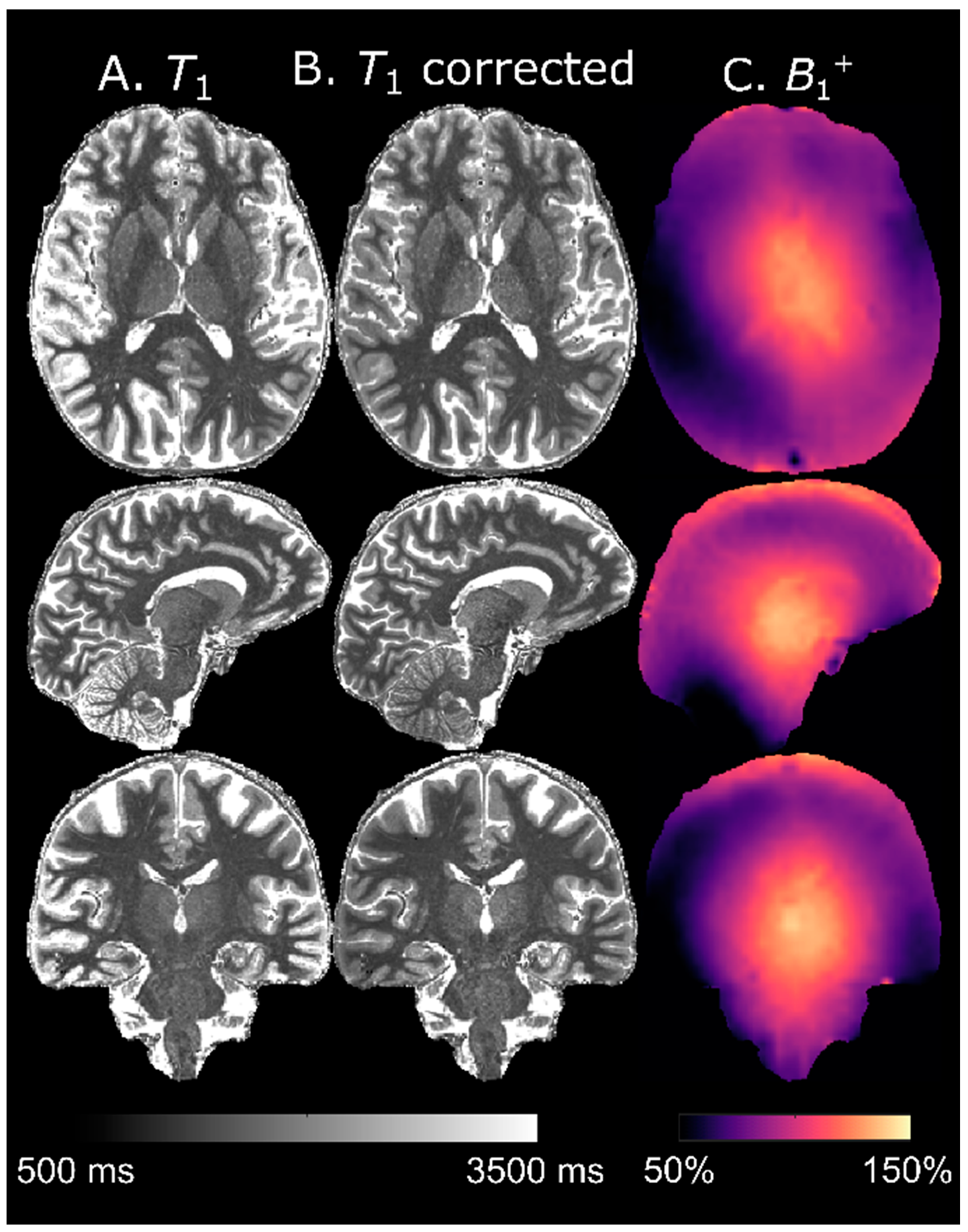
2.12. T1 Calculation

For proof-of-principle, T1-mapping using a LUT-based approach was performed on a healthy subject using the (0.8 mm)3 resolution protocol together with a DREAM flip angle map [
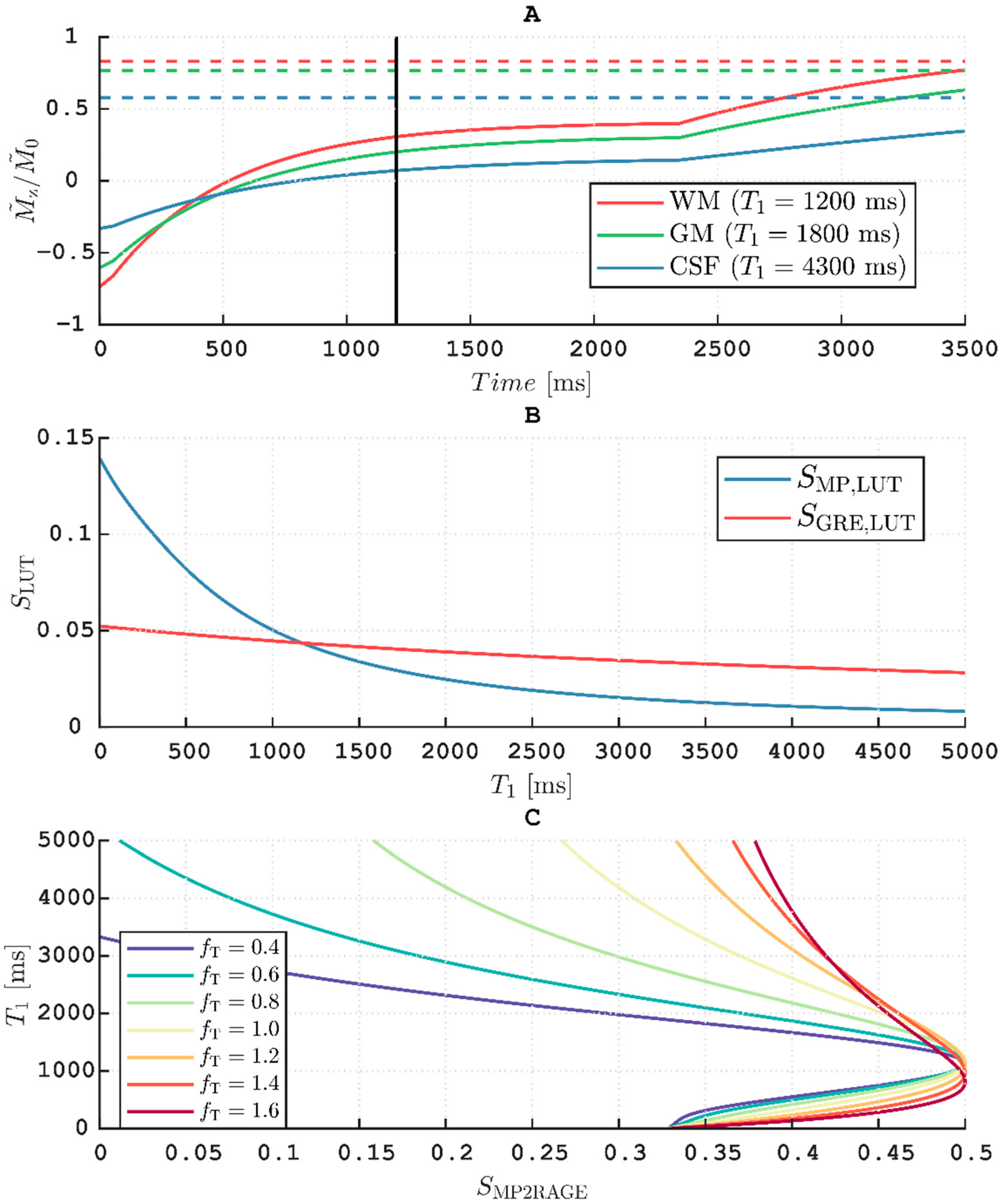
23]. First, the evolution of the longitudinal magnetization, Mz, was simulated for the MPRAGE sequence with imaging parameters as described above, i.e., with αMP = 8°, TR = 8 ms, TI = 1200 ms and TF = 288.
The evolution of Mz during Tcycle in the outer loop steady-state (occurring after 2–3 cycles) was simulated using Equations (2) and (3) in the intervals where readout occurred and using normal T1 relaxation where readout did not occur. The simulations can be performed with M ˜ z (i.e., per unit ρ ). The inversion efficiency applied at the end of each cycle was assumed to be finv = 0.96 [5]. The LUT-derived signal was then calculated for a constant α MP but over a range of f T as:
S MP , LUT = M ˜ z , MP ( f T , T 1 , T I ) M ˜ 0 sin ( f T α MP ) .
The reference GRE was assumed to always be in the inner loop steady-state. Hence, M ˜ z , GRE and consequently the LUT-derived GRE signal, S GRE , LUT , is constant for a constant T 1 and f T :
S GRE , LUT = M ˜ z , GRE ( f T , T 1 ) M ˜ 0 sin ( f T α MP ) .
Thus, 2D ( n T 1 × n f T ) LUTs of S MP , LUT and S GRE , LUT are obtained for a range of 1   s T 1 5   s (step size of 1 ms, n T 1 = 5000 ) and 0.4 f T 1.6 (step size of 0.01, n f T = 121 ). The LUTs of the two simulated signals were then combined as follows [5]:
S MP 2 RAGE , LUT ( T 1 ,   f T ) = S MP , LUT · S GRE , LUT S MP , LUT 2 + S GRE , LUT 2 .
Thus, the values are limited to 0 S MP 2 RAGE , LUT ( T 1 ,   f T ) 0.5 in the final LUT for comparison with S MP 2 RAGE = S MP · S GRE S MP 2 + S GRE 2   calculated from the measured magnitude signals. Note that the measured S MP 2 RAGE ( T 1 ,   f T ) is limited to positive values for this implementation, since it is not possible to relate the phases of two signals measured sequentially. The T 1 for which | S MP 2 RAGE S MP 2 RAGE , LUT | was minimal was calculated pixelwise either for f T = 1 or as determined by the DREAM flip angle map.

3. Results

3.1. Readout Flip Angle of Reference GRE

There was a continuous decrease in tissue contrast in the normalized volume as αGRE increased (Figure 1). This decrease was evident both from visual inspection (for αGRE > 3°) and from the quantitative comparison of segmented WM and GM (panel C). The contrast was still increased after normalization, compared to before, for all values of αGRE. The ROI analysis (panel D) showed no decrease in CV, neither at lower αGRE nor after normalization, and no apparent change in SNR could thus be identified. However, a minimum in the CV of segmented WM (panel E) was observed at αGRE = 3°, implying minimal influence of residual B1+ inhomogeneities at this setting. The B1+ influence was visually identifiable as elevated pixel values in the center of the brain using αGRE = 6° (panel B). Based on these results, and to avoid deviating too far from the Ernst angle (~7°–5° for 1000 ms ≤ T1 ≤ 2000 ms), αGRE = 3° was deemed optimal and chosen for the final protocol. At αGRE = 3°, the WM-GM contrast was C = 0.18 and the variability across segmented WM was CV = 9% after normalization compared to C = 0.10 and CV = 34% before.

3.2. Voxel Size of Reference GRE

Increasing Vref (Figure 2) yielded very similar normalized MPRAGE images (panel B). Although some ringing artifacts were visible in the images (cf. red arrow in panel B), increased Vref did not cause any noticeably stronger effect. No change in WM-GM contrast (C = 0.24 at Vref = 0.7 × 0.7 × 1.4 vs. C = 0.23 at Vref = 2.8 × 2.8 × 1.4) was observed with increasing Vref (panel C). Although a higher SNR is to be expected for larger Vref, no trend in the CV of the WM ROI could be discerned (panel D). A weak trend of increasing CV in segmented WM was observed (CV = 7.3% at Vref = 0.7 × 0.7 × 1.4 vs. CV = 9.5% at Vref = 2.8 × 2.8 × 1.4), possibly reflecting partial volume effects (PVEs) (panel E). No difference between Vref = 0.7 × 0.7 × 1.4 and Vref = 1.4 × 1.4 × 1.4 was discernible. Hence, Vref in one dimension was set to twice that of the MPRAGE voxel size in one dimension, i.e., 1.43/1.63/1.83 mm3 for 0.73/0.83/0.93 mm3, which reduced the total scan time by 71/53/42 s respectively (i.e., a reduction by 14/14/12%). A higher Vref was not employed to avoid more pronounced PVEs and interpolation errors.

3.3. Implementation at Different Resolutions

Figure 3 shows normalized MPRAGE images of the same subject for 0.7 and 0.9-mm isotropic resolution (without elliptical phase encoding). The histograms indicate that signal intensity in GM remains relatively unchanged while WM becomes brighter when the TF is reduced, thus increasing the WM-GM contrast. The reduction in contrast due to higher TF is in concordance with findings by Deichmann et al. [7] No increase in Gibbs ringing at the lower spatial resolution was observed.

3.4. Intra-Subject Variability

The MPRAGE volumes, before and after normalization, are shown in Figure 4. The normalized volumes show a noticeably increased spatial homogeneity. Hyperintense pixel values in the temporal lobes and cerebellum of the normalized volumes are indicative of a failed inversion with the adiabatic pulse [24]. These bright pixel intensities were exacerbated in session #4, possibly due to a transmitter adjustment failure. Before normalization, the average CVs were 20 ± 7.8% in WM, 32 ± 12% in GM and 46 ± 19% in CSF (Figure 5). The corresponding values after normalization were 7.9 ± 3.3% in WM, 15 ± 7.0% in GM and 33 ± 16% in CSF. Exclusion of session #4 yielded an average CV of 16 ± 8.1/27 ± 14/39 ± 24% in WM/GM/CSF before normalization and 7.2 ± 2.5/11 ± 6.8/22 ± 14% after. The results of the ROI-based analysis can be seen in Table 2.

3.5. Inter-Subject Variability

The CV was substantially reduced after normalization also in the inter-subject comparison (Figure 5). This improved reproducibility was most evident in the WM and basal ganglia since the diffeomorphic registration made a pixelwise comparison difficult in the cortex. Before normalization, the average CVs in MNI space were 13 ± 7.8/22 ± 9.5/45 ± 20% in WM/GM/CSF, respectively. The corresponding values after normalization were 7.6 ± 7.6/18 ± 10/43 ± 24%. Based on individual segmentations, the CVs were 6.2/6.5/9.0% before normalization and 2.0/4.3/6.4% after in WM/GM/CSF. Results of the ROI-based analysis can be seen in Table 2.

3.6. Comparison to MP2RAGE

The MP2RAGE image showed a higher WM-GM contrast than the normalized MPRAGE obtained using the (0.7 mm)3 protocol suggested here (Figure 6). The difference in pixel intensity between the WM/GM histogram modes was 0.785 − 0.545 = 0.24 for the normalized MPRAGE compared to 0.275 − (−0.155) = 0.43 for the MP2RAGE. The underlying reason is the larger dynamic range of Mz in MP2RAGE. The interleaved acquisition and complex image combination of the MP2RAGE approach can utilize this as information of the polarity of Mz is retained. The interleaved acquisition of the reference GRE, however, requires a longer Tcycle, which was 5.0 s for MP2RAGE compared to 3.5 s in the sequential protocol. This in turn entails a longer Tacq, which in this case was 8:20 min compared to 5:59 + 1:10 = 7:09 min. The acquisition time of the sequential protocol could have been reduced further to 4:35 + 0:54 = 5:29 min if an elliptical k-space encoding (as was used for the MP2RAGE sequence) had been employed.

3.7. T1 Calculation

The evolution of M ˜ z , MP over Tcycle for TF = 288 is shown in panel A of Figure 7. The LUT signals were derived from this evolution for different T1s and fT = 1 (panel B). The resulting T1 as a function of SMP2RAGE at different fT values is also shown (panel C). For these sequence parameters, the B1+ bias was most pronounced at long T1 (i.e., for CSF). Around approximately 1000 ms, however, T1 was no longer uniquely defined for a given SMP2RAGE, which thus set the lower limit of measurable T1. This lower limit varied, based on fT as 1122/1156/1181/1169/1097/966/810 ms for fT = 0.4/0.6/0.8/1.0/1.2/1.4/1.6, respectively. At fT = 0.4, there was also an upper limit at 3330 ms. Figure 8 shows a map of T1 derived from this LUT before (panel A) and after (panel B) B1+-correction. Estimated tissue T1 was only moderately affected by the B1+-correction although an elevation of T1 in the thalamus (fT ≈ 1.3) after correction can be discerned. The most notable difference was seen in the CSF, which was adjusted toward higher values in high B1+ areas and toward lower values in low B1+ areas. Especially after correction, the distribution of T1 seemed to be very homogenous within different tissues, without any obvious B1+ bias.

3.8. Example Results Using the Finalized Protocol

Figure 9 shows images from a subject using the finalized protocol (0.83 mm3, without elliptical phase encoding). After normalization, effects from the intensity field bias were considerably reduced. For instance, the diagonal B1+ pattern in the axial plane was removed as well as the right–left asymmetry in the coronal plane. The improved homogeneity can also be seen in the whole-brain histogram where WM and GM form distinct modes after normalization. Issues of extremely low B1+ (fT ~ 0.3) in the right part of the cerebellum, where the local flip angle is too low to fulfil the adiabatic condition for inversion, can, however, not be resolved by normalization (red arrow).

4. Discussion

In this study, we describe the process of implementing a sequential protocol for bias field correction of MPRAGE images at 7 T. Effects of varying the flip angle, different spatial resolutions and acquisition voxel size of the reference GRE were studied, mainly to improve WM-GM contrast and to minimize scan time without introducing biases. The main purpose of the protocols was to obtain semi-quantitative images with “pure” T1 contrast and improved reproducibility. Improved intra-subject reproducibility was demonstrated by a decreased CV of 7.9 ± 3.3% in segmented WM after normalization compared to 20 ± 7.8% before. Likewise, an improved inter-subject reproducibility was demonstrated by the CV in segmented WM of 10 subjects which decreased from 13 ± 7.8% to 7.6 ± 7.6%. Local improvement could be higher, for instance 39 ± 3.1% to 7.6 ± 2.2% in frontal WM in the intra-subject experiment and 22 ± 1.4% to 4.4 ± 0.91% in the cerebellum in the inter-subject experiment.
The multiplicative spatial intensity bias imposed by the combination of receive coil signals was removed by normalization. Due to a smaller readout flip angle in the reference GRE compared to the MPRAGE, and to the rather small flip angles overall, the effect of the inhomogeneous transmit field (B1+) was also mostly removed. Since the analytical description of the MPRAGE signal is too complicated to evaluate [25], we estimated T1 maps through a LUT-based approach analogous to MP2RAGE [5]. As expected, accuracy was improved by using a separate B1+ map.
The protocol was not designed with T1 calculation, as featured by MP2RAGE, in mind. Thus, at the rather long TI = 1200 ms the protocol fails to effectively exploit the dynamic range obtained when inverting fully relaxed longitudinal magnetization (cf. Figure 7, panel A). This results in quite “saturated” images when normalizing using Equation (8) (pixels close to 0.5), leading to a loss of precision in the T1 calculation. Further, although whole-brain histograms of T1 were very similar when using different Vref, it is most likely prudent to use identical voxel sizes of MPRAGE and the reference GRE if accurate T1 estimation is of interest, especially at the cortical boundaries that are most susceptible to PVEs. It is important to note that the LUT-based approach assumes that all differences in pixel values are solely caused by variations in T1 (i.e., that there is “pure” T1 contrast). By design, the influence of B1+ inhomogeneities on the T1 calculation is decreased by the normalization of signals. The choice of αMP = 2.7αGRE (8° vs. 3°) appeared to minimize residual effects of B1+ inhomogeneity on the normalized MPRAGE (cf. Figure 1) and thus also on the T1 calculation. The largest residual effect of B1+ inhomogeneity was found at αMP = 1.3αGRE (8° vs. 6°). This is in concordance with the work of Van de Moortele et al. in which a choice of αMP = αGRE resulted in a much stronger residual B1+ dependence than αMP = 2αGRE [4]. To increase accuracy, a separately acquired flip angle map is still recommended if T1-mapping is of interest [26]. This is particularly important for longer T1 values where the B1+ influence is stronger (cf. panel C, Figure 7). The loss of contrast observed in the cerebellum (cf. panel C, Figure 9) occurs when B1+ decreases below the threshold required for the inversion pulse to fulfil the adiabatic condition which cannot be resolved by flip angle mapping [24].
The obvious benefit of an interleaved acquisition is that identical scanning conditions, such as RF power calibration, is guaranteed, as well as increased robustness against inter-scan movement. Inter-scan motion can be corrected by offline rigid coregistration, however. Further, the reduced duration of any one acquisition will reduce the total risk of intra-scan subject movement. The risk of introducing T1 contrast in the GRE reference due to poor timings (mainly TI and/or TF×TR being too short) is also removed [4]. Importantly, the option to increase Vref facilitates the possibility to have a shorter total scan time than needed for the interleaved MP2RAGE.
A protocol with an MPRAGE acquisition voxel size of (0.6 mm)3 was also explored (data not shown). However, the SNR in the MPRAGE was deemed unacceptably low. Hence, the (0.7 mm)3 protocol here represents the upper limit of the spatial resolution imposed by SNR. It should be noted that noise propagation will moderately decrease the SNR in the normalized MPRAGE, S MP / GRE , relative to the unnormalized, S MP , by S MP 1 + S MP / GRE 2 , thereby somewhat adversely affecting obtainable spatial resolution [4]. Decreasing the acquisition voxel size also entails increasing TF and thus the duration of the readout train and eventually of TI. This limitation can be circumvented by introducing a SENSE factor in the inner loop, as shown here for (0.7 mm)3. The employed zigzag k-space trajectory (see the view-ordering schemes presented for turbo spin echoes in ref. [27]) allows the use of a TF larger than the number of inner loop k-space lines (Ny), which is an effective way to decrease scan time. It further allows the enabling of an elliptical k-space phase encoding which decreases the acquisition time by a factor of approximately r 2 / ( π ( r / 2 ) 2 ) 1.3 (cf. Table 1). To our knowledge, this kind of k-space trajectory is only readily available on Philips’s systems. Hence, the total scan time of the protocols are supplied with/without elliptical phase encoding.
Correction of RF field-induced bias is recommended at field strengths of 7 T and above. However, normalization may also be necessary to correct for intensity field bias at 3 T, as the wavelength of the B1 field is approximately 25 cm in brain tissue and thus of the same order of magnitude as the imaged object [28].

5. Limitations

We did not attempt to optimize the point-spread function (PSF) of the MPRAGE sequence, although this will be broadened when signal is acquired during a transient state [8]. At increasing resolution, readouts are appended at the beginning and end of the RAGE trains (cf. Figure 7, panel A). These will compromise the PSF, so the effective spatial resolution will not increase as much as the nominal spatial resolution. The increased change in Mz during acquisition may also influence the WM-GM contrast (cf. Figure 3). In this work, we focused on the reference GRE for normalization, which is acquired entirely in a steady-state and thus does not suffer from such PSF distortions. Further, the PSF cannot be modelled for an elliptical k-space phase encoding, since the trajectory is proprietary.
Like in MP2RAGE, the loss of T1 contrast at very low B1+ (below the threshold for adiabatic inversion) cannot be mended by normalization [22].
Although subdural ringing artifacts did not noticeably increase when using a protocol with lower spatial resolution (cf. Figure 3), curved ringing artifacts were occasionally observed. These were more evident in the reference GRE but could also be seen in MPRAGE. The artifacts appeared to be correlated to subject movement, but this was not confirmed. These artifacts are believed to be related to interpolation of the low spatial resolution (5.5 × 7.4 × 4.0 mm3) SENSE reference scan, acquired prior to the MPRAGE and reference GRE. The artifact was very similar to the “streaky-linear” artifact “type A” described by Sartoretti et al. and showcased in Figure 3, panels (g), (h), and (i) [29].

6. Conclusions

We describe a sequential protocol for correction of RF-induced bias in MPRAGE images by normalization with a reference GRE. Spatial homogeneity and WM-GM contrast were improved after normalization as well as intra- and inter-subject reproducibility. Scan time could be reduced by increasing the voxel size of the reference GRE without appreciably affecting image quality.

Author Contributions

Conceptualization, G.H.; methodology, G.H. and H.O.; software, H.O. and J.L.; validation, H.O.; formal analysis, H.O.; investigation, G.H. and H.O.; data curation, G.H., H.O., and M.N.; writing—original draft preparation, H.O.; writing—review and editing, H.O., G.H., R.W., J.L., and M.N.; visualization, H.O.; supervision, G.H. and R.W.; funding acquisition, G.H. and R.W. All authors have read and agreed to the published version of the manuscript.

Funding

This research was funded by the Swedish Research Council, grant numbers NT-2014-6193 and M-2017-00995. The APC was funded in part by Lund University.

Institutional Review Board Statement

The study was conducted according to the guidelines of the Declaration of Helsinki, and approved by the Regionala Etikprövningsnämden Lund (9 August 2012, protocol code 2012/428).

Informed Consent Statement

Written informed consent was obtained from all subjects prior to each examination.

Data availability statement

Data is openly available at https://openneuro.org/datasets/ds003769 (accessed on 10 September 2021). The inter-subject variability data is available as sub-001 to sub-010 at https://openneuro.org/datasets/ds003508 (accessed on 10 September 2021). Descriptive pulse sequence text files as well as a MATLAB scripts to perform the T1 calculation is available at https://github.com/OlssonHampus/RF_bias_correction_MPRAGE (accessed on 10 September 2021).

Acknowledgments

The authors are indebted to Fredy Visser, Philips Healthcare, for providing the initial MPRAGE protocol. The Lund University Bioimaging Center (LBIC) is acknowledged for experimental resources. The publication was approved in its submitted form by Philips Medical Systems Nederland B.V. in accordance with the research agreement with LBIC.

Conflicts of Interest

The authors declare no conflict of interest. The funders had no role in the design of the study; in the collection, analyses, or interpretation of data; in the writing of the manuscript, or in the decision to publish the results.

References

  1. Mugler, J.P., 3rd; Brookeman, J.R. Three-dimensional magnetization-prepared rapid gradient-echo imaging (3D MP RAGE). Magn. Reson. Med. 1990, 15, 152–157. [Google Scholar] [CrossRef]
  2. Balchandani, P.; Naidich, T.P. Ultra-High-Field MR Neuroimaging. AJNR Am. J. Neuroradiol. 2015, 36, 1204–1215. [Google Scholar] [CrossRef] [PubMed] [Green Version]
  3. Focke, N.K.; Helms, G.; Kaspar, S.; Diederich, C.; Toth, V.; Dechent, P.; Mohr, A.; Paulus, W. Multi-site voxel-based morphometry—Not quite there yet. Neuroimage 2011, 56, 1164–1170. [Google Scholar] [CrossRef]
  4. Van de Moortele, P.F.; Auerbach, E.J.; Olman, C.; Yacoub, E.; Ugurbil, K.; Moeller, S. T1 weighted brain images at 7 Tesla unbiased for Proton Density, T2* contrast and RF coil receive B1 sensitivity with simultaneous vessel visualization. Neuroimage 2009, 46, 432–446. [Google Scholar] [CrossRef] [PubMed] [Green Version]
  5. Marques, J.P.; Kober, T.; Krueger, G.; van der Zwaag, W.; Van de Moortele, P.F.; Gruetter, R. MP2RAGE, a self bias-field corrected sequence for improved segmentation and T1-mapping at high field. Neuroimage 2010, 49, 1271–1281. [Google Scholar] [CrossRef] [PubMed] [Green Version]
  6. Trampel, R.; Bazin, P.L.; Pine, K.; Weiskopf, N. In-vivo magnetic resonance imaging (MRI) of laminae in the human cortex. Neuroimage 2019, 197, 707–715. [Google Scholar] [CrossRef]
  7. Deichmann, R.; Good, C.D.; Josephs, O.; Ashburner, J.; Turner, R. Optimization of 3-D MP-RAGE sequences for structural brain imaging. Neuroimage 2000, 12, 112–127. [Google Scholar] [CrossRef]
  8. Mugler, J.P., 3rd; Brookeman, J.R. Rapid three-dimensional T1-weighted MR imaging with the MP-RAGE sequence. J. Magn. Reson. Imaging 1991, 1, 561–567. [Google Scholar] [CrossRef]
  9. Teeuwisse, W.M.; Brink, W.M.; Webb, A.G. Quantitative assessment of the effects of high-permittivity pads in 7 Tesla MRI of the brain. Magn. Reson. Med. 2012, 67, 1285–1293. [Google Scholar] [CrossRef]
  10. Pruessmann, K.P.; Weiger, M.; Scheidegger, M.B.; Boesiger, P. SENSE: Sensitivity encoding for fast MRI. Magn. Reson. Med. 1999, 42, 952–962. [Google Scholar] [CrossRef]
  11. Li, X.; Morgan, P.S.; Ashburner, J.; Smith, J.; Rorden, C. The first step for neuroimaging data analysis: DICOM to NIfTI conversion. J. Neurosci. Methods 2016, 264, 47–56. [Google Scholar] [CrossRef]
  12. Chenevert, T.L.; Malyarenko, D.I.; Newitt, D.; Li, X.; Jayatilake, M.; Tudorica, A.; Fedorov, A.; Kikinis, R.; Liu, T.T.; Muzi, M.; et al. Errors in Quantitative Image Analysis due to Platform-Dependent Image Scaling. Transl. Oncol. 2014, 7, 65–71. [Google Scholar] [CrossRef] [Green Version]
  13. Jenkinson, M.; Bannister, P.; Brady, M.; Smith, S. Improved optimization for the robust and accurate linear registration and motion correction of brain images. Neuroimage 2002, 17, 825–841. [Google Scholar] [CrossRef]
  14. Jenkinson, M.; Beckmann, C.F.; Behrens, T.E.; Woolrich, M.W.; Smith, S.M. Fsl. Neuroimage 2012, 62, 782–790. [Google Scholar] [CrossRef] [Green Version]
  15. Smith, S.M. Fast robust automated brain extraction. Hum. Brain Mapp. 2002, 17, 143–155. [Google Scholar] [CrossRef]
  16. Zhang, Y.; Brady, M.; Smith, S. Segmentation of brain MR images through a hidden Markov random field model and the expectation-maximization algorithm. IEEE Trans. Med. Imaging 2001, 20, 45–57. [Google Scholar] [CrossRef]
  17. Rooney, W.D.; Johnson, G.; Li, X.; Cohen, E.R.; Kim, S.G.; Ugurbil, K.; Springer, C.S., Jr. Magnetic field and tissue dependencies of human brain longitudinal 1H2O relaxation in vivo. Magn. Reson. Med. 2007, 57, 308–318. [Google Scholar] [CrossRef] [PubMed]
  18. Olsson, H.; Andersen, M.; Latt, J.; Wirestam, R.; Helms, G. Reducing bias in dual flip angle T1-mapping in human brain at 7T. Magn. Reson. Med. 2020, 84, 1347–1358. [Google Scholar] [CrossRef] [Green Version]
  19. Noven, M.; Olsson, H.; Helms, G.; Horne, M.; Nilsson, M.; Roll, M. Cortical and white matter correlates of language-learning aptitudes. Hum. Brain Mapp. 2021. [Google Scholar] [CrossRef] [PubMed]
  20. Ashburner, J. A fast diffeomorphic image registration algorithm. Neuroimage 2007, 38, 95–113. [Google Scholar] [CrossRef] [PubMed]
  21. Tabelow, K.; Balteau, E.; Ashburner, J.; Callaghan, M.F.; Draganski, B.; Helms, G.; Kherif, F.; Leutritz, T.; Lutti, A.; Phillips, C.; et al. hMRI—A toolbox for quantitative MRI in neuroscience and clinical research. Neuroimage 2019. [Google Scholar] [CrossRef] [PubMed]
  22. Helms, G.; Latt, J.; Olsson, H. Cross-vendor transfer and RF coil comparison of a high-resolution MP2RAGE protocol for brain imaging at 7T. Acta Sci. Lund. 2020, 2020, 1–12. [Google Scholar]
  23. Olsson, H.; Andersen, M.; Helms, G. Reducing bias in DREAM flip angle mapping in human brain at 7T by multiple preparation flip angles. Magn. Reson. Imaging 2020, 72, 71–77. [Google Scholar] [CrossRef]
  24. Kadhim, M. Measuring T1 Using MP2RAGE in Human Brain at 7T-Effect of B1+ and Inversion Pulse Efficiency. Master’s Thesis, Lund University, Lund, Sweden, 2021. Available online: https://lup.lub.lu.se/student-papers/search/publication/9043213 (accessed on 10 September 2021).
  25. Wright, P.J.; Mougin, O.E.; Totman, J.J.; Peters, A.M.; Brookes, M.J.; Coxon, R.; Morris, P.E.; Clemence, M.; Francis, S.T.; Bowtell, R.W.; et al. Water proton T1 measurements in brain tissue at 7, 3, and 1.5 T using IR-EPI, IR-TSE, and MPRAGE: Results and optimization. Magn. Reson. Mater. Phys. Biol. Med. 2008, 21, 121–130. [Google Scholar] [CrossRef] [PubMed]
  26. Haast, R.A.M.; Lau, J.C.; Ivanov, D.; Menon, R.S.; Uludag, K.; Khan, A.R. Effects of MP2RAGE B1(+) sensitivity on inter-site T1 reproducibility and hippocampal morphometry at 7T. Neuroimage 2021, 224, 117373. [Google Scholar] [CrossRef]
  27. Busse, R.F.; Brau, A.C.; Vu, A.; Michelich, C.R.; Bayram, E.; Kijowski, R.; Reeder, S.B.; Rowley, H.A. Effects of refocusing flip angle modulation and view ordering in 3D fast spin echo. Magn. Reson. Med. 2008, 60, 640–649. [Google Scholar] [CrossRef] [PubMed] [Green Version]
  28. Gabriel, C. Compilation of the Dielectric Properties of Body Tissues at RF and Microwave Frequencies; King’s College: London, UK, 1996. [Google Scholar]
  29. Sartoretti, T.; Reischauer, C.; Sartoretti, E.; Binkert, C.; Najafi, A.; Sartoretti-Schefer, S. Common artefacts encountered on images acquired with combined compressed sensing and SENSE. Insights Imaging 2018, 9, 1107–1115. [Google Scholar] [CrossRef] [Green Version]
Figure 1. Reference GREs with different αGRE (top row, (A)) used to obtain normalized MPRAGE volumes (middle row, (B)). Decreasing WM-GM contrast with increasing αGRE is evident from visual inspection of the normalized volumes and verified in the scatter plot (C). No change in SNR could be identified by the CV in a WM ROI (red circle) (D). The CV in whole segmented WM had a minimum at αGRE = 3°, implying minimum influence from residual B1+ effects (E). These residual B1+ effects are visually identifiable as hyperintense pixels in the center of the normalized MPRAGE for αGRE = 6° (B). The solid lines in the scatter plots represent the respective MPRAGE volume values before normalization. In this experiment, the dielectric pads caused a visible fold-over artefact (red arrow).
Tomography 07 00038 g001
Figure 2. Reference GREs with different in-plane voxel sizes (top row, (A))) used to obtain normalized MPRAGE (middle row, (B)). The reference GREs and thereby also the normalized MPRAGE volumes are very similar. Some ringing artifacts are visible (red arrow) but do not appear to severely affect image quality even at the lowest resolution in this experiment. Scatter plot of contrast vs. voxel volume (C) shows no change in WM-GM contrast with increasing Vref. No change in SNR could be identified by the CV in a WM ROI (red circle) (D). A slight increase of the CV in the segmented WM is visible at higher Vref, possibly reflecting PVEs (E). The solid lines in the scatter plots represent the respective MPRAGE values before normalization.
Tomography 07 00038 g002
Figure 3. Normalized MPRAGE images acquired on the same subject with two protocols with different resolutions. (A) (0.7 mm)3, and (B) (0.9 mm)3. At 0.9 mm isotropic resolution, WM pixel values are increased (black arrow in histogram plot) relative (0.7 mm)3 while GM pixel values remain largely unaffected, increasing tissue contrast. This is an effect of the shortened readout train (lower TF).
Tomography 07 00038 g003
Figure 4. MPRAGE volumes before (SMP) and after (SMP/GRE) normalization, acquired on a subject scanned at five separate sessions (day 1, 161, 170, 189, and 253). Influence from the bias field is noticeably reduced after normalization. Hyperintense pixels indicate a failed adiabatic inversion. At the 4th scanning session, there was possibly a transmitter adjustment failure, resulting in generally lower B1+ and thus a generally darker SMP image as well as a larger area of very bright pixels in the cerebellumum of SMP/GRE.
Tomography 07 00038 g004
Figure 5. Maps of the CV before and after normalization, showing the intra- and inter-subject variability. The intra-subject CV maps were calculated from data acquired at five scanning sessions under an eight-month period. The inter-subject CV maps, in MNI space, were calculated from data acquired from 10 separate subjects. Reproducibility was improved after normalization in both cases. The ROIs corresponding to the data in Table 2 are denoted in purple in the “Before” maps.
Tomography 07 00038 g005
Figure 6. A normalized MPRAGE image (A) compared to an MP2RAGE image (B) with comparative whole-brain histograms. The MP2RAGE utilizes a larger dynamic range through the interleaved acquisition and complex combination and thus has a higher WM-GM contrast.
Tomography 07 00038 g006
Figure 7. (A) Solid coloured lines show the evolution of Mz during an MPRAGE acquisition across Tcycle = 3500 ms and fT = 1 for three values of T1 exemplifying WM, GM, and CSF. The dashed lines show the corresponding steady-state of the reference GRE. Vertical black line denotes the center of k-space at TI = 1200 ms. (B) The two LUT signals as a function of T1 for fT = 1. (C) Estimated T1 as a function of SMP2RAGE for different fT. Areas with longer T1 were disproportionately biased by deviations in fT. Depending on fT, the minimum T1 that could be uniquely defined ranged from 1181 ms (fT = 0.8) and 810 ms (fT = 1.6). At fT = 0.4, there was also an upper limit at 3330 ms.
Tomography 07 00038 g007
Figure 8. LUT-derived T1 maps, uncorrected (A) and corrected (B) with a separately acquired B1+ map (C). The T1 estimation in tissue was moderately robust against B1+ influence and mostly CSF was affected.
Tomography 07 00038 g008
Figure 9. Example images acquired with the MPRAGE protocol before normalization (A), the reference GRE used for normalization (B), and the MPRAGE image after normalization (C). The right-hand panel shows whole-brain histograms of the respective images. Normalization clearly reduced spatial heterogeneity from B1. The improved homogeneity is also illustrated by the histograms, where GM and WM (and to a lesser extent CSF) modes are visible after normalization. In the right part of the cerebellum (red arrow, coronal plane), B1+ is very weak, leading to failed adiabatic inversion.
Tomography 07 00038 g009
Table 1. Acquisition times (Tacq) of the non-interleaved protocol at different spatial resolutions and with/without elliptical k-space phase encoding. The MPRAGE with (0.7 mm)3 resolution used an inner loop SENSEAP = 1.11 to accommodate the readout train.
Parameter/Resolution(0.7 mm)3(0.8 mm)3(0.9 mm)3
MP Nx,y,z328 × 328 × 257288 × 288 × 225256 × 256 × 200
GRE Nx,y,z164 × 164 × 128144 × 144 × 112128 × 128 × 100
MP TF296288256
MP Tacq (min)05:5905:1404:39
MP Tacq (elliptical) (min)04:3504:0403:36
GRE Tacq (min)01:1000:5300:42
GRE Tacq (elliptical) (min)00:5400:4000:32
Total Tacq (min)07:0906:0705:21
Total Tacq (elliptical) (min)05:4504:5704:18
Table 2. ROI analysis of the CV maps in Figure 5.
ROIIntra-Subject beforeIntra-Subject after NormalizationInter-Subject beforeInter-Subject after
Frontal WM39 ± 3.1%7.6 ± 2.2%9.2 ± 1.4%3.7 ± 1.1%
Caudate head26 ± 2.9%13 ± 3.5%6.8 ± 0.90%3.7 ± 1.2%
Cerebellum21 ± 3.6%8.7 ± 2.9%22 ± 1.4%4.8 ± 0.91%
Temporal lobe34 ± 4.3%9.8 ± 2.3%16 ± 1.8%6.1 ± 1.3%
Publisher’s Note: MDPI stays neutral with regard to jurisdictional claims in published maps and institutional affiliations.

