
A Reinforced Whale Optimization Algorithm for Solving Mathematical Optimization Problems


Abstract

1. Introduction
2. Whale Optimization Algorithm (WOA)
2.1. Exploitation Phase
2.2. Exploration Phase
3. A Reinforced Whale Optimization Algorithm
3.1. Opposition-Based Learning
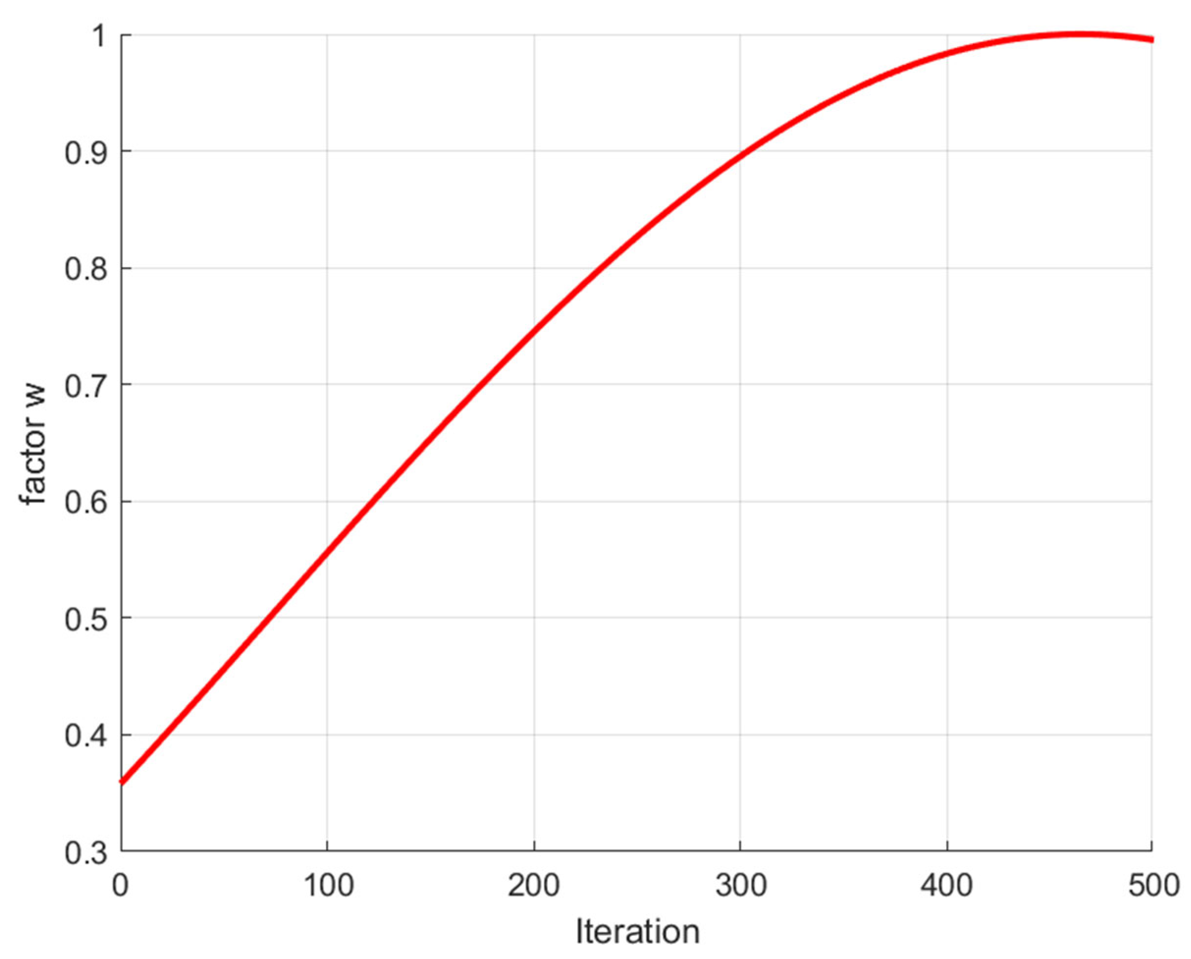
3.2. Adaptive Weight Strategy
3.3. Improved Encircling Prey Mechanics
| Algorithm 1. Pseudo-code of RWOA |
| (i = 1, 2, …, N) are randomly generated within the range of the problem space |
| 2: Each individual is assigned a value to the corresponding pbest. Calculate the fitness value of all individuals, find the best fitness value, and assign it to gbest. |
| 3: Initialize the parameters a, A, C, l, p, w |
| 4: t = 0 |
| 5: While t < Tmax do |
| 6: if p < 0.5 |
| 7: if |A| < 1 |
| 8: Update each individual position using Equations (5) and (8) |
| 9: else if |A| ≥ 1 |
| 10: Select a random search agent Xrand |
| 11: Update each individual position using Equations (1) and (2) |
| 12: end if |
| 13: else if p ≥ 0.5 |
| 14: Update each individual position using Equation (6) and (ii) in Equation (7) |
| 15: end if |
| 16: Update the individual historical optimal position pbest and its fitness value |
| 17: Update the best optimal position gbest using the opposition-based learning strategy, Equation (3); calculate the fitness value, and select the one with the best fitness value to reassign it to gbest |
| 18: Boundary checks and adjustments |
| 19: t = t + 1 |
| 20: Update the parameters a, A, C, l, p, w |
| 21: end while |
| 22: Output the global best solution (gbest) |
3.4. Space Complexity Analysis
4. Performance Testing of RWOA and WOA
4.1. Performance Testing on 23 Benchmark Functions
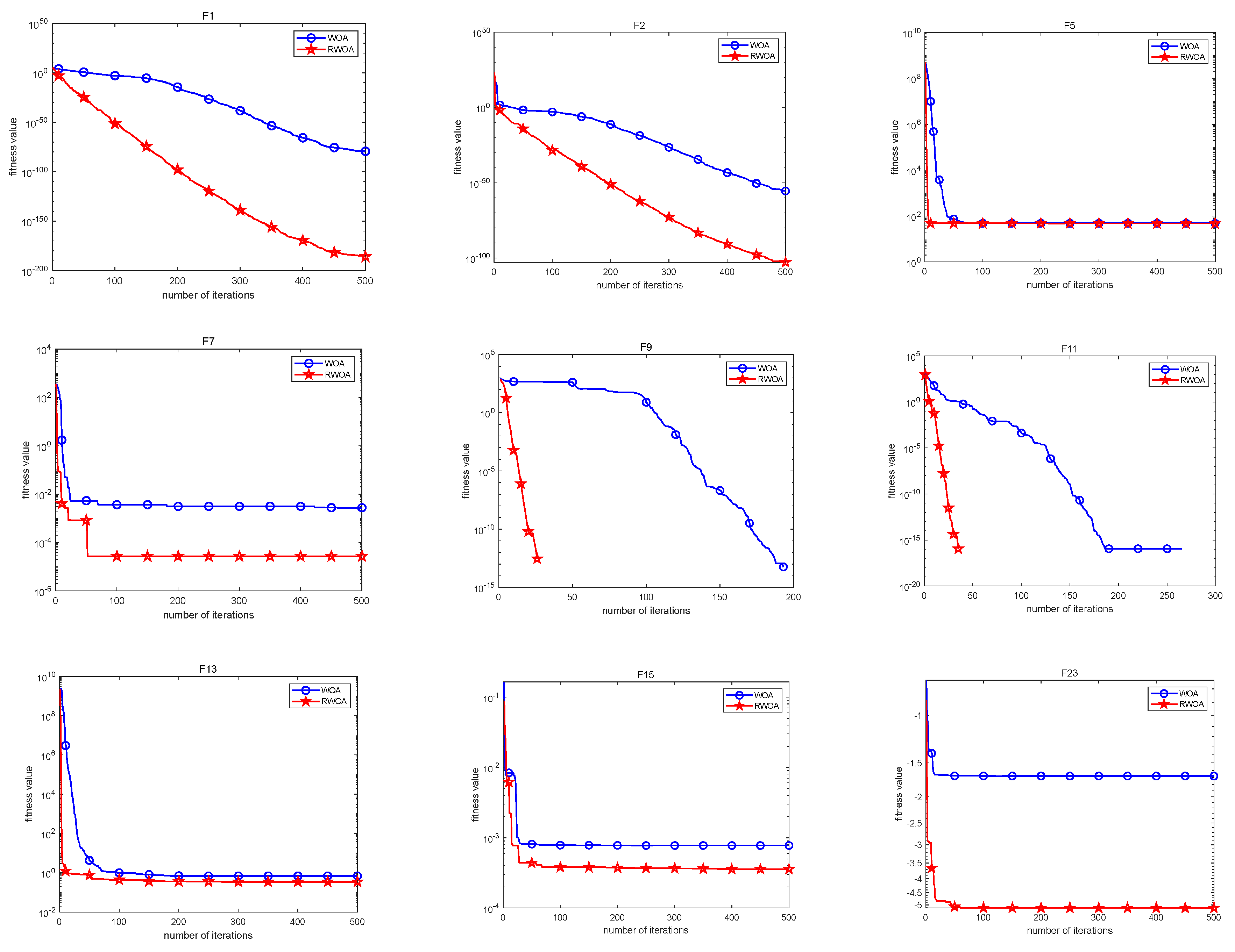
4.1.1. Exploitation Capability Evaluation through Uni-Modal Functions
4.1.2. Exploration Ability Evaluation through Multi-Modal Functions
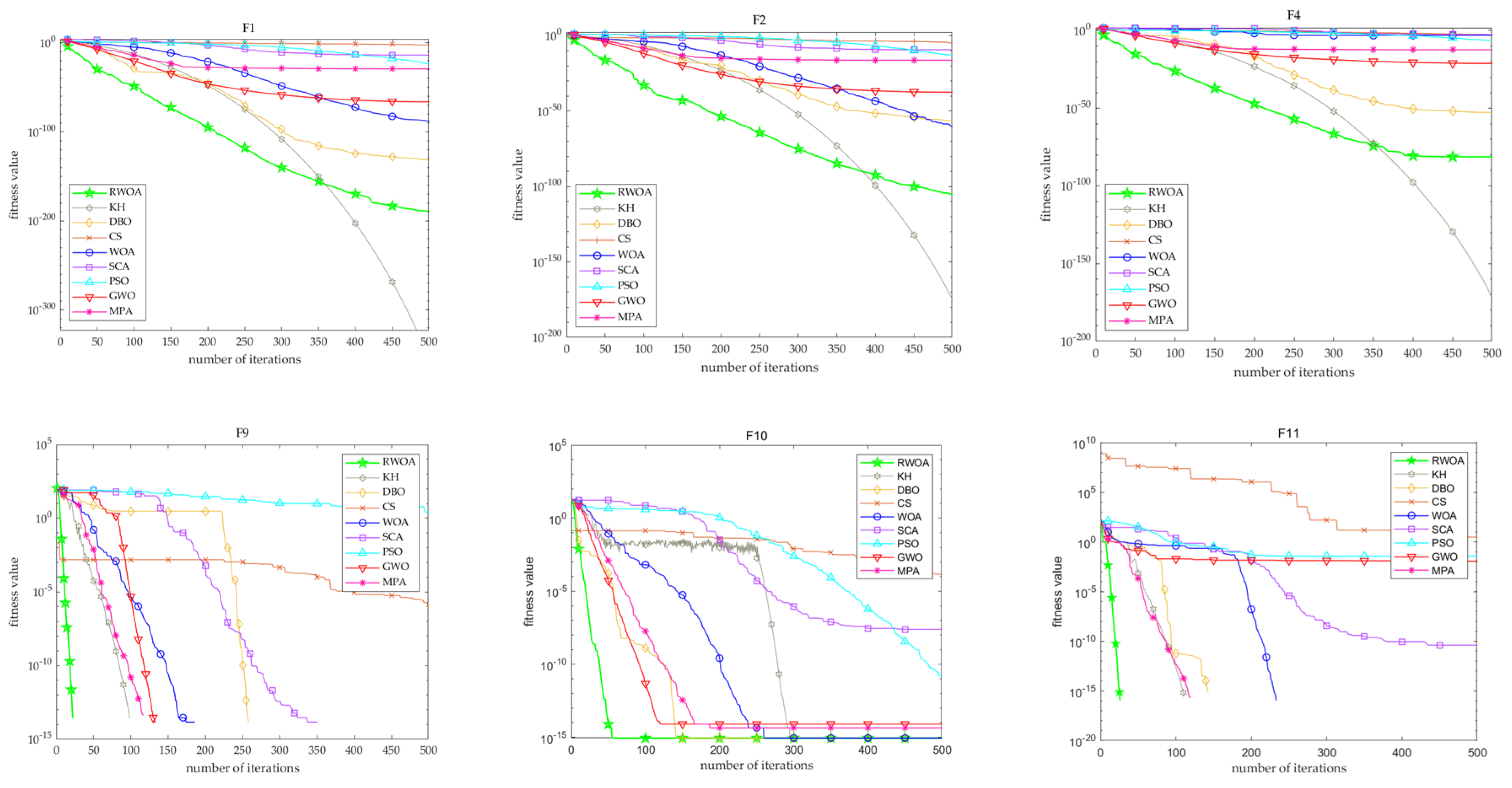
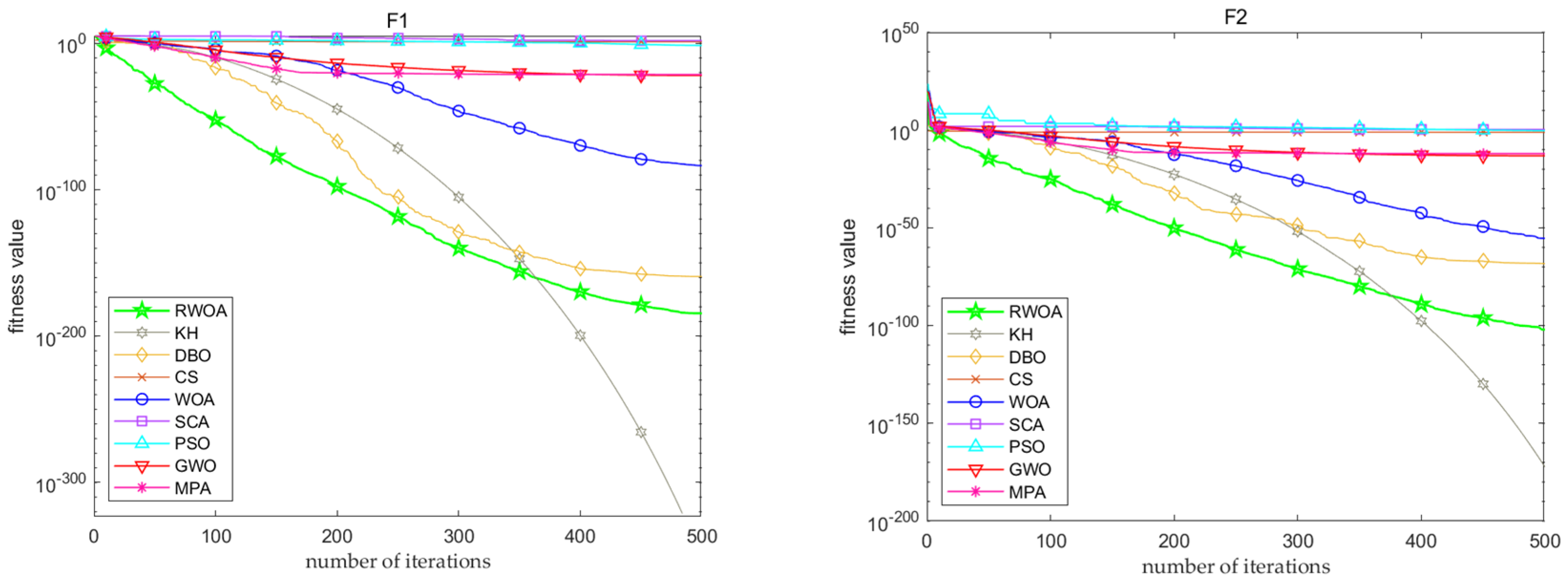
4.1.3. Analysis of Statistical Test and Convergence Performance
4.2. Performance Testing on CEC-2017
4.3. Performance Testing on CEC-2022
5. Comparison of Performance with Other Algorithms
5.1. Compare with TSA and ABC
5.2. Comparison of the Performance of RWOA with Multiple Algorithms
6. Discussions
7. Conclusions
Author Contributions
Funding
Data Availability Statement
Conflicts of Interest
References
- Kennedy, J.; Eberhart, R. Particle swarm optimization. In Proceedings of the International Conference on Neural Networks (ICNN’95), Perth, WA, Australia, 27 November–1 December 1995; Volume 4, pp. 1942–1948. [Google Scholar]
- Karaboga, D. An Idea Based on Honey Bee Swarm for Numerical Optimization; Erciyes University: Kayseri, Turkey, 2005. [Google Scholar]
- Yang, X.S.; Deb, S. Cuckoo Search via Lévy Flights. In Proceedings of the 2009 World Congress on Nature & Biologically Inspired Computing (NaBIC), Coimbatore, India, 9–11 December 2009; pp. 210–214. [Google Scholar]
- Gandomi, A.H.; Alavi, A.H. Krill herd: A new bio-inspired optimization algorithm. Commun. Nonlinear Sci. Numer. Simul. 2012, 17, 4831–4845. [Google Scholar] [CrossRef]
- Mirjalili, S.; Mirjalili, S.M.; Lewis, A. Grey wolf optimizer. Adv. Eng. Softw. 2014, 69, 46–61. [Google Scholar] [CrossRef]
- Kiran, M.S. TSA: Tree-seed algorithm for continuous optimization. Expert Syst. Appl. 2015, 42, 6686–6698. [Google Scholar] [CrossRef]
- Mirjalili, S. SCA: A sine cosine algorithm for solving optimization problems. Knowl. Based Syst. 2016, 96, 120–133. [Google Scholar] [CrossRef]
- Mirjalili, S.; Lewis, A. The whale optimization algorithm. Adv. Eng. Softw. 2016, 95, 51–67. [Google Scholar] [CrossRef]
- Faramarzi, A.; Heidarinejad, M.; Mirjalili, S.; Gandomi, A.H. Marine Predators Algorithm: A nature-inspired metaheuristic. Expert Syst. Appl. 2020, 152, 113377. [Google Scholar] [CrossRef]
- Xue, J.; Shen, B. Dung beetle optimizer: A new meta-heuristic algorithm for global optimization. J. Supercomput. 2023, 79, 7305–7336. [Google Scholar] [CrossRef]
- Tawhid, M.A.; Ibrahim, A.M. Feature selection based on rough set approach, wrapper approach, and binary whale optimization algorithm. Int. J. Mach. Learn. Cybern. 2020, 11, 573–602. [Google Scholar] [CrossRef]
- Mafarja, M.; Thaher, T.; Al-Betar, M.A.; Too, J.; Awadallah, M.A.; Abu Doush, I.; Turabieh, H. Classification framework for faulty-software using enhanced exploratory whale optimizer-based feature selection scheme and random forest ensemble learning. Appl. Intell. 2023, 53, 18715–18757. [Google Scholar] [CrossRef]
- Jiang, T.; Zhang, C.; Sun, Q.M. Green job shop scheduling problem with discrete whale optimization algorithm. IEEE Access 2019, 7, 43153–43166. [Google Scholar] [CrossRef]
- Liu, M.; Yao, X.; Li, Y. Hybrid whale optimization algorithm enhanced with Lévy flight and differential evolution for job shop scheduling problems. Appl. Soft Comput. 2020, 87, 105954. [Google Scholar] [CrossRef]
- Zhao, F.; Xu, Z.; Bao, H.; Xu, T.; Zhu, N. A cooperative whale optimization algorithm for energy-efficient scheduling of the distributed blocking flow-shop with sequence-dependent setup time. Comput. Ind. Eng. 2023, 178, 109082. [Google Scholar] [CrossRef]
- Ewees, A.A.; Abd Elaziz, M.; Oliva, D. A new multi-objective optimization algorithm combined with opposition-based learning. Expert Syst. Appl. 2021, 165, 113844. [Google Scholar] [CrossRef]
- Ma, G.; Yue, X. An improved whale optimization algorithm based on multilevel threshold image segmentation using the Otsu method. Eng. Appl. Artif. Intell. 2022, 113, 104960. [Google Scholar] [CrossRef]
- Agrawal, S.; Panda, R.; Choudhury, P.; Abraham, A. Dominant color component and adaptive whale optimization algorithm for multilevel thresholding of color images. Knowl. Based Syst. 2022, 240, 108172. [Google Scholar] [CrossRef]
- Sun, Y.; Wang, X.; Chen, Y.; Liu, Z. A modified whale optimization algorithm for large-scale global optimization problems. Expert Syst. Appl. 2018, 114, 563–577. [Google Scholar] [CrossRef]
- Chen, H.; Yang, C.; Heidari, A.A.; Zhao, X. An efficient double adaptive random spare reinforced whale optimization algorithm. Expert Syst. Appl. 2020, 154, 113018. [Google Scholar] [CrossRef]
- Lee, C.Y.; Zhuo, G.L. A hybrid whale optimization algorithm for global optimization. Mathematics 2021, 9, 1477. [Google Scholar] [CrossRef]
- Prasad, D.; Mukherjee, A.; Mukherjee, V. Temperature dependent optimal power flow using chaotic whale optimization algorithm. Expert Syst. 2021, 38, e12685. [Google Scholar] [CrossRef]
- Sun, Y.; Chen, Y. Multi-population improved whale optimization algorithm for high dimensional optimization. Appl. Soft Comput. 2021, 112, 107854. [Google Scholar] [CrossRef]
- Li, Y.; Li, W.G.; Zhao, Y.T.; Liu, A. Opposition-based multi-objective whale optimization algorithm with multi-leader guiding. Soft Comput. 2021, 25, 15131–15161. [Google Scholar] [CrossRef]
- Islam, Q.N.U.; Ahmed, A.; Abdullah, S.M. Optimized controller design for islanded microgrid using non-dominated sorting whale optimization algorithm (NSWOA). Ain Shams Eng. J. 2021, 12, 3677–3689. [Google Scholar] [CrossRef]
- Saha, N.; Panda, S. Cosine adapted modified whale optimization algorithm for control of switched reluctance motor. Comput. Intell. 2022, 38, 978–1017. [Google Scholar] [CrossRef]
- Liu, J.; Shi, J.; Hao, F.; Dai, M. A novel enhanced global exploration whale optimization algorithm based on Lévy flights and judgment mechanism for global continuous optimization problems. Eng. Comput. 2023, 39, 2433–2461. [Google Scholar] [CrossRef]
- Jin, H.; Lv, S.; Yang, Z.; Liu, Y. Eagle strategy using uniform mutation and modified whale optimization algorithm for QoS-aware cloud service composition. Appl. Soft Comput. 2022, 114, 108053. [Google Scholar] [CrossRef]
- Yang, X.S.; Deb, S. Eagle strategy using Lévy walk and firefly algorithms for stochastic optimization. In Nature Inspired Cooperative Strategies for Optimization (NICSO 2010); Springer: Berlin/Heidelberg, Germany, 2010; pp. 101–111. [Google Scholar]
- Guo, Q.; Gao, L.; Chu, X.; Sun, H. Parameter identification for static var compensator model using sensitivity analysis and improved whale optimization algorithm. CSEE J. Power Energy Syst. 2022, 8, 535–547. [Google Scholar]
- Lin, X.; Yu, X.; Li, W. A heuristic whale optimization algorithm with niching strategy for global multi-dimensional engineering optimization. Comput. Ind. Eng. 2022, 171, 108361. [Google Scholar] [CrossRef]
- Zong, X.; Liu, J.; Ye, Z.; Liu, Y. Whale optimization algorithm based on Levy flight and memory for static smooth path planning. Int. J. Mod. Phys. C 2022, 33, 2250138. [Google Scholar] [CrossRef]
- Zhou, R.; Zhang, Y.; He, K. A novel hybrid binary whale optimization algorithm with chameleon hunting mechanism for wrapper feature selection in QSAR classification model: A drug-induced liver injury case study. Expert Syst. Appl. 2023, 234, 121015. [Google Scholar] [CrossRef]
- Shen, Y.; Zhang, C.; Gharehchopogh, F.S.; Mirjalili, S. An improved whale optimization algorithm based on multi-population evolution for global optimization and engineering design problems. Expert Syst. Appl. 2023, 215, 119269. [Google Scholar] [CrossRef]
- Wolpert, D.H.; Macready, W.G. No free lunch theorems for optimization. IEEE Trans. Evol. Comput. 1997, 1, 67–82. [Google Scholar] [CrossRef]
- Shekhawat, S.; Saxena, A. Development and applications of an intelligent crow search algorithm based on opposition based learning. ISA Trans. 2020, 99, 210–230. [Google Scholar] [CrossRef] [PubMed]
- Abdel-Basset, M.; Mohamed, R.; Mirjalili, S.; Chakrabortty, R.K.; Ryan, M.J. MOEO-EED: A multi-objective equilibrium optimizer with exploration–exploitation dominance strategy. Knowl. Based Syst. 2021, 214, 106717. [Google Scholar] [CrossRef]
- Yuan, J.; Zhao, Z.; Liu, Y.; He, B.; Wang, L.; Xie, B.; Gao, Y. DMPPT control of photovoltaic microgrid based on improved sparrow search algorithm. IEEE Access 2021, 9, 16623–16629. [Google Scholar] [CrossRef]
- Ouyang, C.; Zhu, D.; Qiu, Y. Lens Learning Sparrow Search Algorithm. Math. Probl. Eng. 2021, 2021, 9935090. [Google Scholar] [CrossRef]
- Jiao, J.; Cheng, J.; Liu, Y.; Yang, H.; Tan, D.; Cheng, P.; Zhang, Y.; Jiang, C.; Chen, Z. Inversion of TEM measurement data via a quantum particle swarm optimization algorithm with the elite opposition-based learning strategy. Comput. Geosci. 2023, 174, 105334. [Google Scholar] [CrossRef]
- Han, B.; Li, B.; Qin, C. A novel hybrid particle swarm optimization with marine predators. Swarm Evol. Comput. 2023, 83, 101375. [Google Scholar] [CrossRef]
- Jensi, R.; Jiji, G.W. An enhanced particle swarm optimization with levy flight for global optimization. Appl. Soft Comput. 2016, 43, 248–261. [Google Scholar] [CrossRef]
- Zhang, C.; Ding, S. A stochastic configuration network based on chaotic sparrow search algorithm. Knowl. Based Syst. 2021, 220, 106924. [Google Scholar] [CrossRef]
- Ma, Y.; Zhang, X.; Song, J.; Chen, L. A modified teaching–learning-based optimization algorithm for solving optimization problem. Knowl. Based Syst. 2021, 212, 106599. [Google Scholar] [CrossRef]
- Ma, Y.; Chang, C.; Lin, Z.; Zhang, X.; Song, J.; Chen, L. Modified Marine Predators Algorithm hybridized with teaching-learning mechanism for solving optimization problems. Math. Biosci. Eng. 2022, 20, 93–127. [Google Scholar] [CrossRef] [PubMed]
- Ferahtia, S.; Houari, A.; Rezk, H.; Djerioui, A.; Machmoum, M.; Motahhir, S.; Ait-Ahmed, M. Red-tailed hawk algorithm for numerical optimization and real-world problems. Sci. Rep. 2023, 13, 12950. [Google Scholar] [CrossRef] [PubMed]
- Liang, J.J.; Qin, A.K.; Suganthan, P.N.; Baskar, S. Comprehensive learning particle swarm optimizer for global optimization of multimodal functions. IEEE Trans. Evol. Comput. 2006, 10, 281–295. [Google Scholar] [CrossRef]
- Cheng, R.; Jin, Y. A social learning particle swarm optimization algorithm for scalable optimization. Inf. Sci. 2015, 291, 43–60. [Google Scholar] [CrossRef]


| Algorithm | Pros and Cons | Year | Refs. |
|---|---|---|---|
| PSO | It has a strong global search ability and fast convergence speed, but it easily falls into the local optimal solution. | 1995 | [1] |
| ABC | A good balance of exploration and exploitation capabilities. However, it converges slowly and is sensitive to parameter configurations. | 2005 | [2] |
| CS | The model is simple, has few parameters, and is highly versatile, but it easily falls into local optimum. | 2009 | [3] |
| KHA | Strong global search ability, fast convergence speed, and good robustness. | 2012 | [4] |
| GWO | Its parameters are few, and the convergence speed is fast, but the algorithm easily matures early, and the convergence accuracy is low. | 2014 | [5] |
| TSA | It is easy to operate and provides a good balance between exploration and development capabilities. However, it is very sensitive to parameter selection and incurs high computational costs for high-dimensional problems. | 2015 | [6] |
| SCA | The structure is simple, and the calculation efficiency is high, but the convergence accuracy is low. | 2016 | [7] |
| WOA | The operation is simple, the control parameters are few, and the ability to jump out of the local optimum is strong, but the optimization speed is slow, the accuracy is low, and the exploration and development ability of the algorithm is poor. | 2016 | [8] |
| MPA | It has few parameters, has a simple structure, and is easy to implement with high calculation accuracy, but it easily falls into the local optimum and has a poor balance of mining and exploration, poor convergence speed, and solution quality. | 2020 | [9] |
| DBO | It has strong stability, fast search speed, and high accuracy, but it easily falls into the local optimum. | 2022 | [10] |
| Tactics | Update Formulas | Condition |
|---|---|---|
| encircling prey | p < 0.5, |A| < 1 | |
| bubble net attack | p ≥ 0.5 | |
| Functions | RWOA | WOA | |||||||
|---|---|---|---|---|---|---|---|---|---|
| Max | Mean | Min | SD | Max | Mean | Min | SD | p-Values | |
| F1 | 2.36 × 10−180 | 1.12 × 10−181 | 4.68 × 10−196 | 0.00 | 4.38 × 10−80 | 1.52 × 10−81 | 4.63 × 10−90 | 7.99 × 10−81 | 1.73 × 10⁻⁶ |
| F2 | 7.59 × 10−101 | 3.10 × 10−102 | 6.03 × 10−107 | 1.40 × 10−101 | 9.61 × 10−52 | 5.07 × 10−53 | 3.71 × 10−59 | 1.84 × 10−52 | 1.73 × 10⁻⁶ |
| F3 | 1.25 × 10−121 | 4.43 × 10−123 | 4.01 × 10−143 | 2.29 × 10−122 | 2.38 × 10⁵ | 1.74 × 10⁵ | 1.10 × 10⁵ | 3.58 × 10⁴ | 1.73 × 10⁻⁶ |
| F4 | 2.95 × 10−72 | 9.90 × 10−74 | 1.24 × 10−83 | 5.39 × 10−73 | 92.30 | 61.30 | 0.28 | 30.8 | 1.73 × 10⁻⁶ |
| F5 | 48.20 | 47.60 | 46.90 | 0.31 | 48.60 | 47.90 | 47.00 | 0.43 | 5.32 × 10⁻³ |
| F6 | 0.81 | 0.45 | 6.76 × 10⁻² | 0.18 | 1.62 | 0.72 | 0.14 | 0.29 | 1.89 × 10⁻⁴ |
| F7 | 1.81 × 10⁻⁴ | 4.36 × 10⁻⁵ | 9.05 × 10⁻⁶ | 4.17 × 10⁻⁵ | 1.82 × 10⁻² | 4.38 × 10⁻³ | 7.87 × 10⁻⁶ | 4.90 × 10⁻³ | 1.92 × 10⁻⁶ |
| Function | RWOA | WOA | |||||||
|---|---|---|---|---|---|---|---|---|---|
| Max | Mean | Min | SD | Max | Mean | Min | SD | p-Values | |
| F8 | −2.00 × 10⁴ | −2.09 × 10⁴ | −2.09 × 10⁴ | 2.26 × 10² | −1.26 × 10⁴ | −1.72 × 10⁴ | −2.09 × 10⁴ | 2.80 × 10³ | 1.73 × 10⁻⁶ |
| F9 | 0.00 | 0.00 | 0.00 | 0.00 | 0.00 | 0.00 | 0.00 | 0.00 | 1.00 |
| F10 | 8.88 × 10⁻¹⁶ | 8.88 × 10⁻¹⁶ | 8.88 × 10⁻¹⁶ | 0.00 | 7.99 × 10⁻¹⁵ | 4.91 × 10⁻¹⁵ | 8.88 × 10⁻¹⁶ | 2.23 × 10⁻¹⁵ | 3.17 × 10⁻⁶ |
| F11 | 0.00 | 0.00 | 0.00 | 0.00 | 0.21 | 2.15 × 10⁻² | 0.00 | 5.74 × 10⁻² | 0.13 |
| F12 | 2.40 × 10⁻² | 1.27 × 10⁻² | 1.49 × 10⁻⁴ | 5.57 × 10⁻³ | 3.51 × 10⁻² | 1.51 × 10⁻² | 6.04 × 10⁻³ | 7.27 × 10⁻³ | 0.22 |
| F13 | 0.62 | 0.31 | 6.74 × 10⁻² | 0.14 | 1.76 | 0.78 | 0.28 | 0.32 | 2.35 × 10⁻⁶ |
| Function | RWOA | WOA | |||||||
|---|---|---|---|---|---|---|---|---|---|
| RWOA | WOA | ||||||||
| Max | Mean | Min | SD | Max | Mean | Min | SD | p-Values | |
| F14 | 10.80 | 1.82 | 1.00 | 1.87 | 10.80 | 2.96 | 1.00 | 3.25 | 0.15 |
| F15 | 6.35 × 10⁻⁴ | 3.32 × 10⁻⁴ | 3.08 × 10⁻⁴ | 6.45 × 10⁻⁵ | 7.64 × 10⁻³ | 8.64 × 10⁻⁴ | 3.10 × 10⁻⁴ | 1.34 × 10⁻³ | 4.73 × 10⁻⁶ |
| F16 | −1.03 | −1.03 | −1.03 | 4.35 × 10⁻⁶ | −1.03 | −1.03 | −1.03 | 8.74 × 10⁻¹⁰ | 1.73 × 10⁻⁶ |
| F17 | 0.40 | 0.40 | 0.40 | 2.15 × 10⁻⁵ | 0.40 | 0.40 | 0.40 | 1.32 × 10⁻⁵ | 1.75 × 10⁻² |
| F18 | 3.00 | 3.00 | 3.00 | 1.16 × 10⁻⁴ | 3.00 | 3.00 | 3.00 | 5.42 × 10⁻⁵ | 0.67 |
| F19 | −3.85 | −3.86 | −3.86 | 2.69 × 10⁻³ | −3.850 | −3.86 | −3.86 | 4.69 × 10⁻³ | 0.13 |
| F20 | −3.02 | −3.21 | −3.32 | 9.51 × 10⁻² | −3.05 | −3.21 | −3.32 | 9.57 × 10⁻² | 0.88 |
| F21 | −5.05 | −7.11 | −10.2 | 2.45 | −2.63 | −8.46 | −10.20 | 2.68 | 1.11 × 10⁻² |
| F22 | −5.08 | −6.97 | −10.4 | 2.52 | −2.77 | −7.79 | −10.40 | 3.08 | 0.26 |
| F23 | −5.12 | −7.25 | −10.5 | 2.57 | −1.68 | −7.83 | −10.50 | 3.25 | 5.45 × 10⁻² |
| Function | RWOA | WOA | |||||||
|---|---|---|---|---|---|---|---|---|---|
| Max | Mean | Min | SD | Max | Mean | Min | SD | p-Values | |
| CECF1 | 6.02 × 10⁹ | 2.08 × 10⁹ | 4.24 × 10⁸ | 1.07 × 10⁹ | 4.99 × 10⁸ | 4.15 × 10⁷ | 3.81 × 10⁶ | 9.18 × 10⁷ | 1.73 × 10⁻⁶ |
| CECF3 | 6.91 × 10³ | 3.06 × 10³ | 1.57 × 10³ | 1.22 × 10³ | 3.71 × 10⁴ | 6.54 × 10³ | 7.37 × 10² | 7.83 × 10³ | 9.78 × 10⁻² |
| CECF4 | 6.51 × 10² | 4.99 × 10² | 4.16 × 10² | 58.00 | 6.15 × 10² | 4.49 × 10² | 4.01 × 10² | 59.70 | 2.26 × 10³ |
| CECF5 | 5.92 × 10² | 5.70 × 10² | 5.48 × 10² | 11.90 | 6.23 × 10² | 5.60 × 10² | 5.18 × 10² | 22.70 | 5.98 × 10⁻² |
| CECF6 | 6.62 × 10² | 6.37 × 10² | 6.08 × 10² | 10.90 | 6.95 × 10² | 6.42 × 10² | 6.17 × 10² | 16.90 | 0.13 |
| CECF7 | 8.30 × 10² | 7.96 × 10² | 7.66 × 10² | 14.40 | 8.72 × 10² | 7.85 × 10² | 7.46 × 10² | 30.00 | 5.98 × 10⁻² |
| CECF8 | 8.62 × 10² | 8.37 × 10² | 8.26 × 10² | 7.71 | 8.76 × 10² | 8.46 × 10² | 8.19 × 10² | 16.90 | 1.75 × 10⁻² |
| CECF9 | 1.52 × 10³ | 1.29 × 10³ | 1.03 × 10³ | 1.30 × 10² | 2.94 × 10³ | 1.64 × 10³ | 1.09 × 10³ | 5.01 × 10² | 5.71 × 10⁻⁴ |
| CECF10 | 2.82 × 10³ | 2.17 × 10³ | 1.42 × 10³ | 3.41 × 10² | 2.91 × 10³ | 2.21 × 10³ | 1.51 × 10³ | 3.72 × 10² | 0.59 |
| CECF11 | 1.31 × 10³ | 1.22 × 10³ | 1.14 × 10³ | 43.70 | 1.57 × 10³ | 1.26 × 10³ | 1.13 × 10³ | 1.12 × 10² | 0.12 |
| CECF12 | 1.62 × 10⁷ | 6.33 × 10⁶ | 1.44 × 10⁵ | 3.94 × 10⁶ | 2.23 × 10⁷ | 6.63 × 10⁶ | 9.59 × 10⁴ | 7.00 × 10⁶ | 0.89 |
| CECF13 | 3.59 × 10⁴ | 1.15 × 10⁴ | 3.04 × 10³ | 7.62 × 10³ | 3.46 × 10⁴ | 1.33 × 10⁴ | 2.07 × 10³ | 1.11 × 10⁴ | 0.37 |
| CECF14 | 5.17 × 10³ | 2.22 × 10³ | 1.50 × 10³ | 9.61 × 10² | 5.95 × 10³ | 2.85 × 10³ | 1.49 × 10³ | 1.67 × 10³ | 0.36 |
| CECF15 | 1.93 × 10⁴ | 6.15 × 10³ | 1.65 × 10³ | 4.26 × 10³ | 4.85 × 10⁴ | 1.26 × 10⁴ | 2.59 × 10³ | 9.97 × 10³ | 1.04 × 10⁻³ |
| CECF16 | 2.24 × 10³ | 1.98 × 10³ | 1.73 × 10³ | 99.60 | 2.17 × 10³ | 1.90 × 10³ | 1.64 × 10³ | 1.49 × 10² | 2.30 × 10⁻² |
| CECF17 | 1.83 × 10³ | 1.80 × 10³ | 1.76 × 10³ | 15.80 | 1.94 × 10³ | 1.83 × 10³ | 1.75 × 10³ | 57.20 | 6.04 × 10⁻³ |
| CECF18 | 3.72 × 10⁴ | 1.35 × 10⁴ | 3.30 × 10³ | 9.31 × 10³ | 4.25 × 10⁴ | 2.04 × 10⁴ | 3.30 × 10³ | 1.19 × 10⁴ | 2.18 × 10⁻² |
| CECF19 | 6.24 × 10⁵ | 1.03 × 10⁵ | 6.38 × 10³ | 1.44 × 10⁵ | 1.37 × 10⁶ | 9.76 × 10⁴ | 2.00 × 10³ | 2.58 × 10⁵ | 0.17 |
| CECF20 | 2.30 × 10³ | 2.19 × 10³ | 2.11 × 10³ | 48.30 | 2.35 × 10³ | 2.20 × 10³ | 2.05 × 10³ | 76.80 | 0.69 |
| CECF21 | 2.37 × 10³ | 2.25 × 10³ | 2.21 × 10³ | 40.60 | 2.38 × 10³ | 2.34 × 10³ | 2.22 × 10³ | 47.90 | 8.19 × 10⁻⁵ |
| CECF22 | 2.62 × 10³ | 2.42 × 10³ | 2.31 × 10³ | 94.40 | 4.00 × 10³ | 2.43 × 10³ | 2.24 × 10³ | 4.16 × 10² | 1.11 × 10⁻³ |
| CECF23 | 2.70 × 10³ | 2.67 × 10³ | 2.64 × 10³ | 16.40 | 2.70 × 10³ | 2.65 × 10³ | 2.62 × 10³ | 19.50 | 7.71 × 10⁻⁴ |
| CECF24 | 2.81 × 10³ | 2.75 × 10³ | 2.55 × 10³ | 78.20 | 2.85 × 10³ | 2.79 × 10³ | 2.76 × 10³ | 24.70 | 5.32 × 10⁻³ |
| CECF25 | 3.28 × 10³ | 3.06 × 10³ | 2.95 × 10³ | 93.70 | 2.97 × 10³ | 2.94 × 10³ | 2.68 × 10³ | 52.80 | 4.73 × 10⁻⁶ |
| CECF26 | 4.12 × 10³ | 3.33 × 10³ | 2.82 × 10³ | 2.79 × 10² | 4.68 × 10³ | 3.62 × 10³ | 2.88 × 10³ | 5.74 × 10² | 1.48 × 10⁻² |
| CECF27 | 3.24 × 10³ | 3.14 × 10³ | 3.11 × 10³ | 33.60 | 3.24 × 10³ | 3.15 × 10³ | 3.09 × 10³ | 43.40 | 0.72 |
| CECF28 | 3.74 × 10³ | 3.49 × 10³ | 3.18 × 10³ | 1.13 × 10² | 3.74 × 10³ | 3.48 × 10³ | 3.22 × 10³ | 1.66 × 10² | 0.86 |
| CECF29 | 3.60 × 10³ | 3.36 × 10³ | 3.25 × 10³ | 76.00 | 3.73 × 10³ | 3.41 × 10³ | 3.17 × 10³ | 1.18 × 10² | 0.13 |
| CECF30 | 3.88 × 10⁶ | 6.53 × 10⁵ | 5.35 × 10⁴ | 9.29 × 10⁵ | 6.04 × 10⁶ | 1.47 × 10⁶ | 5.82 × 10³ | 1.49 × 10⁶ | 1.96 × 10⁻² |
| Function | WOA | RWOA | |||
|---|---|---|---|---|---|
| Mean | SD | Mean | SD | p-Values | |
| CF1 | 2.19 × 10⁴ | 9.96 × 10³ | 2.40 × 10³ | 9.83 × 10² | 1.73 × 10⁻⁶ |
| CF2 | 4.53 × 10² | 58.50 | 5.52 × 10² | 1.14 × 10² | 1.15 × 10⁻⁴ |
| CF3 | 6.40 × 10² | 13.30 | 6.35 × 10² | 10.80 | 1.75 × 10⁻² |
| CF4 | 8.41 × 10² | 13.30 | 8.34 × 10² | 5.40 | 4.70 × 10⁻³ |
| CF5 | 1.47 × 10³ | 3.70 × 10² | 1.35 × 10³ | 1.80 × 10² | 0.27 |
| CF6 | 4.67 × 10³ | 1.68 × 10³ | 2.14 × 10⁴ | 3.13 × 10⁴ | 1.60 × 10⁻⁴ |
| CF7 | 2.07 × 10³ | 22.90 | 2.10 × 10³ | 26.90 | 7.16 × 10⁻⁴ |
| CF8 | 2.23 × 10³ | 7.69 | 2.23 × 10³ | 5.82 | 3.60 × 10⁻³ |
| CF9 | 2.61 × 10³ | 50.40 | 2.63 × 10³ | 40.40 | 0.15 |
| CF10 | 2.63 × 10³ | 2.55 × 10² | 2.57 × 10³ | 79.60 | 0.47 |
| CF11 | 2.98 × 10³ | 91.30 | 2.96 × 10³ | 2.58 × 10² | 0.57 |
| CF12 | 2.90 × 10³ | 45.30 | 2.90 × 10³ | 25.80 | 0.85 |
| TSA [6] | ABC [6] | WOA | RWOA | |||||
|---|---|---|---|---|---|---|---|---|
| Mean | SD | Mean | SD | Mean | SD | Mean | SD | |
| TF1 | 7.64 × 10−243 | 0.00 | 2.25 × 10⁻¹⁷ | 8.00 × 10⁻¹⁸ | 7.33 × 10−89 | 2.86 × 10−88 | 2.14 × 10−190 | 0.00 |
| TF2 | 3.49 × 10−147 | 1.75 × 10−146 | 7.76 × 10⁻¹⁷ | 2.06 × 10⁻¹⁷ | 3.65 × 10−59 | 1.30 × 10−58 | 6.86 × 10−106 | 3.53 × 10−105 |
| TF3 | 9.47 × 10−63 | 5.15 × 10−62 | 2.08 × 10⁻¹⁴ | 4.56 × 10⁻¹⁴ | 9.70 × 10⁻⁵ | 3.28 × 10⁻⁴ | 1.05 × 10−78 | 3.98 × 10−78 |
| TF4 | 3.33 × 10⁻² | 0.18 | 0.00 | 0.00 | 7.64 × 10⁻⁶ | 1.00 × 10⁻⁵ | 1.34 × 10⁻⁴ | 2.02 × 10⁻⁴ |
| TF5 | 5.16 × 10⁻⁴ | 3.05 × 10⁻⁴ | 2.39 × 10⁻³ | 1.22 × 10⁻³ | 1.20 × 10⁻³ | 1.30 × 10⁻³ | 5.75 × 10⁻⁵ | 8.73 × 10⁻⁵ |
| TF6 | 0.32 | 1.05 | 3.42 × 10⁻² | 3.57 × 10⁻² | 1.88 | 3.63 | 1.21 | 0.50 |
| TF7 | 0.00 | 0.00 | 0.00 | 0.00 | 0.00 | 0.00 | 0.00 | 0.00 |
| TF8 | 2.02 × 10⁻² | 1.57 × 10⁻² | 1.23 × 10⁻³ | 2.80 × 10⁻³ | 4.65 × 10⁻² | 9.47 × 10⁻² | 0.00 | 0.00 |
| TF9 | 7.11 × 10⁻¹⁶ | 1.45 × 10⁻¹⁵ | 3.20 × 10⁻¹⁵ | 1.08 × 10⁻¹⁵ | 3.49 × 10⁻¹⁵ | 1.85 × 10⁻¹⁵ | 8.88 × 10⁻¹⁶ | 0.00 |
| TF10 | 9.42 × 10⁻³² | 3.34 × 10−47 | 0.21 | 8.82 × 10⁻¹⁸ | 3.11 × 10⁻⁴ | 0.00 | 1.85 × 10⁻⁴ | 1.92 × 10⁻⁴ |
| Algorithm | Parameters | Year | Refs. |
|---|---|---|---|
| PSO | 1995 | [1] | |
| CS | pa = 0.25, | 2009 | [3] |
| KHA | 2012 | [4] | |
| GWO | , linearly decrease | 2014 | [5] |
| SCA | 2016 | [7] | |
| WOA | b = 1, , linearly decrease | 2016 | [8] |
| MPA | P = 0.5, FADs = 0.2 | 2020 | [9] |
| DBO | b = 0.3, k = 0.1, S = 0.5, P_percent = 0.2 | 2022 | [10] |
| Function | Parameters | CS | DBO | GWO | KH | PSO | SCA | WOA | MPA | RWOA |
|---|---|---|---|---|---|---|---|---|---|---|
| F1 | Mean | 2.71 × 10⁻³ | 1.26 × 10−104 | 2.49 × 10−64 | 0.00 | 7.01 × 10⁻²³ | 1.33 × 10⁻¹² | 9.30 × 10−85 | 4.85 × 10⁻³⁰ | 2.36 × 10−181 |
| SD | 1.71 × 10⁻³ | 6.91 × 10−104 | 8.63 × 10−64 | 0.00 | 1.66 × 10⁻²² | 3.94 × 10⁻¹² | 2.70 × 10−84 | 6.15 × 10⁻³⁰ | 0.00 | |
| p-values | 1.73 × 10⁻⁶ | 1.73 × 10⁻⁶ | 1.73 × 10⁻⁶ | 1.73 × 10⁻⁶ | 1.73 × 10⁻⁶ | 1.73 × 10⁻⁶ | 1.73 × 10⁻⁶ | 1.73 × 10⁻⁶ | NA | |
| F2 | Mean | 2.28 × 10⁻⁵ | 1.11 × 10−51 | 9.00 × 10−37 | 2.81 × 10−170 | 6.34 × 10⁻¹³ | 1.17 × 10⁻⁹ | 1.88 × 10−54 | 3.29 × 10⁻¹⁷ | 6.86 × 10−105 |
| SD | 3.44 × 10⁻⁵ | 6.05 × 10−51 | 2.11 × 10−36 | 0.00 | 8.23 × 10⁻¹³ | 3.29 × 10⁻⁹ | 6.81 × 10−54 | 3.85 × 10⁻¹⁷ | 1.94 × 10−104 | |
| p-values | 1.73 × 10⁻⁶ | 1.73 × 10⁻⁶ | 1.73 × 10⁻⁶ | 1.73 × 10⁻⁶ | 1.73 × 10⁻⁶ | 1.73 × 10⁻⁶ | 1.73 × 10⁻⁶ | 1.73 × 10⁻⁶ | NA | |
| F3 | Mean | 3.29 × 10⁻³ | 7.59 × 10−81 | 1.19 × 10⁻²⁷ | 0.00 | 3.26 × 10⁻⁷ | 2.10 × 10⁻³ | 1.85 × 10² | 3.03 × 10⁻¹⁴ | 1.25 × 10−138 |
| SD | 3.15 × 10⁻³ | 4.16 × 10−80 | 6.32 × 10⁻²⁷ | 0.00 | 6.30 × 10⁻⁷ | 8.88 × 10⁻³ | 4.17 × 10² | 6.51 × 10⁻¹⁴ | 6.86 × 10−138 | |
| p-values | 1.73 × 10⁻⁶ | 2.88 × 10⁻⁶ | 1.73 × 10⁻⁶ | 1.73 × 10⁻⁶ | 1.73 × 10⁻⁶ | 1.73 × 10⁻⁶ | 1.73 × 10⁻⁶ | 1.73 × 10⁻⁶ | NA | |
| F4 | Mean | 2.09 × 10⁻³ | 9.85 × 10−48 | 9.58 × 10⁻²¹ | 6.79 × 10−165 | 2.52 × 10⁻⁶ | 4.59 × 10⁻⁴ | 0.68 | 1.16 × 10⁻¹² | 2.07 × 10−77 |
| SD | 1.73 × 10⁻³ | 5.39 × 10−47 | 1.38 × 10⁻²⁰ | 0.00 | 3.19 × 10⁻⁶ | 8.99 × 10⁻⁴ | 1.62 | 1.02 × 10⁻¹² | 7.49 × 10−77 | |
| p-values | 1.73 × 10⁻⁶ | 2.60 × 10⁻⁶ | 1.73 × 10⁻⁶ | 1.73 × 10⁻⁶ | 1.73 × 10⁻⁶ | 1.73 × 10⁻⁶ | 1.73 × 10⁻⁶ | 1.73 × 10⁻⁶ | NA | |
| F5 | Mean | 1.89 × 10⁻⁴ | 4.58 | 6.50 | 8.59 | 8.71 | 7.37 | 6.63 | 1.56 | 6.75 |
| SD | 2.92 × 10⁻⁴ | 0.82 | 0.56 | 2.96 × 10⁻² | 1.5.60 | 0.29 | 0.62 | 0.38 | 0.47 | |
| p-values | 1.73 × 10⁻⁶ | 1.92 × 10⁻⁶ | 7.19 × 10⁻² | 1.73 × 10⁻⁶ | 0.15 | 4.07 × 10⁻⁵ | 0.60 | 1.73 × 10⁻⁶ | NA | |
| F6 | Mean | 2.68 × 10⁻³ | 3.36 × 10⁻³² | 3.05 × 10⁻⁶ | 0.96 | 5.70 × 10⁻²³ | 0.41 | 3.64 × 10⁻⁴ | 1.13 × 10⁻¹² | 6.05 × 10⁻³ |
| SD | 2.15 × 10⁻³ | 6.84 × 10⁻³² | 1.12 × 10⁻⁶ | 0.29 | 1.29 × 10⁻²² | 0.11 | 2.96 × 10⁻⁴ | 8.15 × 10⁻¹³ | 4.23 × 10⁻³ | |
| p-values | 1.59 × 10⁻³ | 1.73 × 10⁻⁶ | 1.73 × 10⁻⁶ | 1.73 × 10⁻⁶ | 1.73 × 10⁻⁶ | 1.73 × 10⁻⁶ | 1.73 × 10⁻⁶ | 1.73 × 10⁻⁶ | NA | |
| F7 | Mean | 1.65 × 10⁻⁷ | 1.05 × 10⁻³ | 5.65 × 10⁻⁴ | 9.90 × 10⁻⁵ | 6.11 × 10⁻³ | 2.02 × 10⁻³ | 1.78 × 10⁻³ | 7.35 × 10⁻⁴ | 7.35 × 10⁻⁵ |
| SD | 1.42 × 10⁻⁷ | 5.64 × 10⁻⁴ | 4.47 × 10⁻⁴ | 7.15 × 10⁻⁵ | 2.95 × 10⁻³ | 1.54 × 10⁻³ | 2.12 × 10⁻³ | 4.73 × 10⁻⁴ | 9.56 × 10⁻⁵ | |
| p-values | 1.73 × 10⁻⁶ | 1.73 × 10⁻⁶ | 3.52 × 10⁻⁶ | 8.59 × 10⁻² | 1.73 × 10⁻⁶ | 1.73 × 10⁻⁶ | 1.73 × 10⁻⁶ | 2.13 × 10⁻⁶ | NA | |
| F8 | Mean | 0.61 | −3.63 × 10³ | −2.74 × 10³ | −1.59 × 10³ | −2.42 × 10³ | −2.20 × 10³ | −3.45 × 10³ | −3.57 × 10³ | −4.07 × 10³ |
| SD | 0.52 | 4.47 × 10² | 2.71 × 10² | 3.19 × 10² | 3.31 × 10² | 1.62 × 10² | 5.89 × 10² | 2.16 × 10² | 2.74 × 10² | |
| p-values | 1.73 × 10⁻⁶ | 6.32 × 10⁻⁵ | 1.92 × 10⁻⁶ | 1.73 × 10⁻⁶ | 1.73 × 10⁻⁶ | 1.73 × 10⁻⁶ | 6.32 × 10⁻⁵ | 6.34 × 10⁻⁶ | NA | |
| F9 | Mean | 2.77 × 10⁻⁶ | 1.38 | 0.10 | 0.12 | 0.00 | 5.15 | 0.24 | 0.71 | 0.00 |
| SD | 1.86 × 10⁻⁶ | 4.47 | 0.56 | 0.56 | 0.00 | 3.27 | 1.32 | 3.87 | 0.00 | |
| p-values | 1.73 × 10⁻⁶ | 0.13 | 0.25 | 1.00 | 1.73 × 10⁻⁶ | 2.69 × 10⁻⁵ | 1.00 | 0.50 | NA | |
| F10 | Mean | 1.50 × 10⁻⁴ | 8.88 × 10⁻¹⁶ | 6.81 × 10⁻¹⁵ | 8.88 × 10⁻¹⁶ | 6.02 × 10⁻¹² | 2.43 × 10⁻⁷ | 5.03 × 10⁻¹⁵ | 5.27 × 10⁻¹⁵ | 8.88 × 10⁻¹⁶ |
| SD | 9.47 × 10⁻⁵ | 0.00 | 1.70 × 10⁻¹⁵ | 0.00 | 7.74 × 10⁻¹² | 5.67 × 10⁻⁷ | 2.30 × 10⁻¹⁵ | 1.53 × 10⁻¹⁵ | 0.00 | |
| p-values | 1.73 × 10⁻⁶ | 1.00 | 6.25 × 10⁻⁷ | 1.00 | 1.73 × 10⁻⁶ | 1.73 × 10⁻⁶ | 3.56 × 10⁻⁶ | 4.00 × 10⁻⁷ | NA | |
| F11 | Mean | 1.05 | 2.34 × 10⁻² | 3.51 × 10⁻² | 0.00 | 0.23 | 7.88 × 10⁻² | 4.16 × 10⁻² | 0.00 | 0.00 |
| SD | 0.90 | 5.33 × 10⁻² | 6.51 × 10⁻² | 0.00 | 0.16 | 0.14 | 8.49 × 10⁻² | 0.00 | 0.00 | |
| p-values | 1.73 × 10⁻⁶ | 1.56 × 10⁻² | 8.86 × 10⁻⁵ | 1.00 | 1.73 × 10⁻⁶ | 1.73 × 10⁻⁶ | 7.81 × 10⁻³ | 1.00 | NA | |
| F12 | Mean | 4.51 × 10⁻⁴ | 5.19 × 10⁻¹² | 3.92 × 10⁻³ | 0.36 | 1.33 × 10⁻²⁴ | 8.97 × 10⁻² | 5.03 × 10⁻³ | 5.06 × 10⁻¹³ | 2.55 × 10⁻³ |
| SD | 3.15 × 10⁻⁴ | 2.83 × 10⁻¹¹ | 7.98 × 10⁻³ | 0.22 | 3.77 × 10⁻²⁴ | 3.05 × 10⁻² | 8.99 × 10⁻³ | 3.86 × 10⁻¹³ | 2.11 × 10⁻³ | |
| p-values | 4.29 × 10⁻⁶ | 1.73 × 10⁻⁶ | 0.16 | 1.73 × 10⁻⁶ | 1.73 × 10⁻⁶ | 1.73 × 10⁻⁶ | 0.54 | 1.73 × 10⁻⁶ | NA | |
| F13 | Mean | 5.27 × 10⁻⁴ | 3.75 × 10⁻⁴ | 3.39 × 10⁻³ | 0.76 | 1.62 × 10⁻²² | 0.28 | 1.55 × 10⁻² | 3.22 × 10⁻¹² | 1.67 × 10⁻² |
| SD | 3.60 × 10⁻⁴ | 2.00 × 10⁻³ | 1.85 × 10⁻² | 0.18 | 6.35 × 10⁻²² | 8.24 × 10⁻² | 2.92 × 10⁻² | 3.16 × 10⁻¹² | 1.16 × 10⁻² | |
| p-values | 1.73 × 10⁻⁶ | 1.73 × 10⁻⁶ | 3.11 × 10⁻⁵ | 1.73 × 10⁻⁶ | 1.73 × 10⁻⁶ | 1.73 × 10⁻⁶ | 5.71 × 10⁻² | 1.73 × 10⁻⁶ | NA |
| Function | Parameters | CS | DBO | GWO | KH | PSO | SCA | WOA | MPA | RWOA |
|---|---|---|---|---|---|---|---|---|---|---|
| F1 | Mean | 1.86 × 10² | 1.72 × 10−108 | 3.46 × 10⁻²² | 0.00 | 9.18 × 10⁻² | 5.71 × 10² | 2.89 × 10−79 | 1.69 × 10⁻²⁰ | 2.04 × 10−180 |
| SD | 9.51 × 10² | 9.44 × 10−108 | 2.68 × 10⁻²² | 0.00 | 8.33 × 10⁻² | 7.49 × 10² | 1.13 × 10−78 | 1.51 × 10⁻²⁰ | 0.00 | |
| p-values | 1.73 × 10⁻⁶ | 1.73 × 10⁻⁶ | 1.73 × 10⁻⁶ | 1.73 × 10⁻⁶ | 1.73 × 10⁻⁶ | 1.73 × 10⁻⁶ | 1.73 × 10⁻⁶ | 1.73 × 10⁻⁶ | NA | |
| F2 | Mean | 0.10 | 2.49 × 10−57 | 1.21 × 10⁻¹³ | 4.63 × 10−171 | 0.89 | 0.56 | 2.31 × 10−52 | 4.69 × 10⁻¹² | 4.65 × 10−102 |
| SD | 0.11 | 1.25 × 10−56 | 6.37 × 10⁻¹⁴ | 0.00 | 0.49 | 0.58 | 6.12 × 10−52 | 4.11 × 10⁻¹² | 1.24 × 10−101 | |
| p-values | 1.73 × 10⁻⁶ | 1.73 × 10⁻⁶ | 1.73 × 10⁻⁶ | 1.73 × 10⁻⁶ | 1.73 × 10⁻⁶ | 1.73 × 10⁻⁶ | 1.73 × 10⁻⁶ | 1.73 × 10⁻⁶ | NA | |
| F3 | Mean | 15.60 | 8.44 × 10⁻¹³ | 3.84 × 10⁻² | 0.00 | 1.21 × 10³ | 4.38 × 10⁴ | 1.77 × 10⁵ | 0.13 | 1.55 × 10−121 |
| SD | 17.80 | 4.62 × 10⁻¹² | 6.26 × 10⁻² | 0.00 | 3.25 × 10² | 1.36 × 10⁴ | 3.56 × 10⁴ | 0.28 | 8.46 × 10−121 | |
| p-values | 1.73 × 10⁻⁶ | 4.29 × 10⁻⁶ | 1.73 × 10⁻⁶ | 1.73 × 10⁻⁶ | 1.73 × 10⁻⁶ | 1.73 × 10⁻⁶ | 1.73 × 10⁻⁶ | 1.73 × 10⁻⁶ | NA | |
| F4 | Mean | 7.86 × 10² | 1.11 × 10−50 | 9.06 × 10⁻⁵ | 3.02 × 10−167 | 3.27 | 68.10 | 59.90 | 3.53 × 10⁻⁸ | 9.18 × 10−75 |
| SD | 4.24 × 10³ | 6.08 × 10−50 | 6.86 × 10⁻⁵ | 0.00 | 0.52 | 7.22 | 28.50 | 1.37 × 10⁻⁸ | 3.46 × 10−74 | |
| p-values | 1.73 × 10⁻⁶ | 1.73 × 10⁻⁶ | 1.73 × 10⁻⁶ | 1.73 × 10⁻⁶ | 1.73 × 10⁻⁶ | 1.73 × 10⁻⁶ | 1.73 × 10⁻⁶ | 1.73 × 10⁻⁶ | NA | |
| F5 | Mean | 0.98 | 45.70 | 47.30 | 48.50 | 3.27 × 10² | 3.50 × 10⁶ | 48.00 | 46.20 | 47.70 |
| SD | 1.42 | 0.25 | 0.82 | 1.51 × 10⁻² | 2.10 × 10² | 4.08 × 10⁶ | 0.39 | 0.51 | 0.30 | |
| p-values | 1.73 × 10⁻⁶ | 1.73 × 10⁻⁶ | 6.87 × 10⁻² | 1.92 × 10⁻⁶ | 1.73 × 10⁻⁶ | 1.73 × 10⁻⁶ | 1.48 × 10⁻⁴ | 1.92 × 10⁻⁶ | NA | |
| F6 | Mean | 9.43 | 1.58 × 10⁻² | 2.25 | 10.60 | 7.24 × 10⁻² | 4.34 × 10² | 0.69 | 0.27 | 0.47 |
| SD | 16.10 | 3.69 × 10⁻² | 0.56 | 0.68 | 3.85 × 10⁻² | 4.25 × 10² | 0.21 | 0.16 | 0.25 | |
| p-values | 5.79 × 10⁻⁵ | 1.73 × 10⁻⁶ | 1.73 × 10⁻⁶ | 1.73 × 10⁻⁶ | 1.92 × 10⁻⁶ | 1.73 × 10⁻⁶ | 2.96 × 10⁻³ | 6.64 × 10⁻⁴ | NA | |
| F7 | Mean | 1.46 × 10⁻³ | 2.09 × 10⁻³ | 2.49 × 10⁻³ | 1.11 × 10⁻⁴ | 1.85 | 3.47 | 2.66 × 10⁻³ | 9.50 × 10⁻⁴ | 4.27 × 10⁻⁵ |
| SD | 1.29 × 10⁻³ | 1.25 × 10⁻³ | 9.91 × 10⁻⁴ | 9.99 × 10⁻⁵ | 0.78 | 4.23 | 2.84 × 10⁻³ | 5.65 × 10⁻⁴ | 3.63 × 10⁻⁵ | |
| p-values | 2.88 × 10⁻⁶ | 1.73 × 10⁻⁶ | 1.73 × 10⁻⁶ | 8.31 × 10⁻⁴ | 1.73 × 10⁻⁶ | 1.73 × 10⁻⁶ | 1.73 × 10⁻⁶ | 1.73 × 10⁻⁶ | NA | |
| F8 | Mean | 7.19 × 10⁶ | −1.41 × 10⁴ | −9.14 × 10³ | −3.34 × 10³ | −7.53 × 10³ | −4.87 × 10³ | −1.86 × 10⁴ | −1.33 × 10⁴ | −2.06 × 10⁴ |
| SD | 1.89 × 10⁷ | 2.64 × 10³ | 1.26 × 10³ | 6.65 × 10² | 2.31 × 10³ | 3.71 × 10² | 2.72 × 10³ | 7.24 × 10² | 8.46 × 10² | |
| p-values | 1.73 × 10⁻⁶ | 1.73 × 10⁻⁶ | 1.73 × 10⁻⁶ | 1.73 × 10⁻⁶ | 1.73 × 10⁻⁶ | 1.73 × 10⁻⁶ | 4.20 × 10⁻⁴ | 1.73 × 10⁻⁶ | NA | |
| F9 | Mean | 2.68 × 10⁻² | 1.26 | 2.49 | 0.00 | 1.40 × 10² | 1.08 × 10² | 0.00 | 0.00 | 0.00 |
| SD | 2.37 × 10⁻² | 4.82 | 2.95 | 0.00 | 33.50 | 63.00 | 0.00 | 0.00 | 0.00 | |
| p-values | 1.73 × 10⁻⁶ | 0.50 | 1.73 × 10⁻⁶ | 1.00 | 1.73 × 10⁻⁶ | 1.73 × 10⁻⁶ | 1.00 | 1.00 | NA | |
| F10 | Mean | 1.17 | 8.88 × 10⁻¹⁶ | 3.19 × 10⁻¹² | 8.88 × 10⁻¹⁶ | 1.44 | 1.89 × 101 | 4.20 × 10⁻¹⁵ | 1.89 × 10⁻¹¹ | 8.88 × 10⁻¹⁶ |
| SD | 1.39 | 0.00 | 1.73 × 10⁻¹² | 0.00 | 0.57 | 4.54 | 2.27 × 10⁻¹⁵ | 1.05 × 10⁻¹¹ | 0.00 | |
| p-values | 1.73 × 10⁻⁶ | 1.00 | 1.73 × 10⁻⁶ | 1.00 | 1.73 × 10⁻⁶ | 1.73 × 10⁻⁶ | 8.19 × 10⁻⁶ | 1.73 × 10⁻⁶ | NA | |
| F11 | Mean | 5.10 × 10⁷ | 0.00 | 3.31 × 10⁻³ | 0.00 | 6.86 × 10⁻³ | 4.93 | 0.00 | 0.00 | 0.00 |
| SD | 1.27 × 10⁸ | 0.00 | 7.15 × 10⁻³ | 0.00 | 7.87 × 10⁻³ | 2.68 | 0.00 | 0.00 | 0.00 | |
| p-values | 1.73 × 10⁻⁶ | 1.00 | 7.81 × 10⁻³ | 1.00 | 1.73 × 10⁻⁶ | 1.73 × 10⁻⁶ | 1.00 | 1.00 | NA | |
| F12 | Mean | 2.02 | 2.30 × 10⁻³ | 0.11 | 1.01 | 2.26 × 10⁻² | 1.44 × 10⁷ | 1.74 × 10⁻² | 6.73 × 10⁻³ | 1.07 × 10⁻² |
| SD | 2.02 | 1.14 × 10⁻² | 9.51 × 10⁻² | 0.13 | 5.52 × 10⁻² | 2.43 × 10⁷ | 1.03 × 10⁻² | 5.39 × 10⁻³ | 5.96 × 10⁻³ | |
| p-values | 1.73 × 10⁻⁶ | 3.11 × 10⁻⁵ | 1.73 × 10⁻⁶ | 1.73 × 10⁻⁶ | 7.19 × 10⁻² | 1.73 × 10⁻⁶ | 9.27 × 10⁻³ | 1.29 × 10⁻³ | NA | |
| F13 | Mean | 2.21 | 1.34 | 1.84 | 4.94 | 8.34 × 10⁻² | 1.34 × 10⁷ | 0.83 | 0.38 | 0.25 |
| SD | 1.93 | 0.73 | 0.31 | 1.57 × 10⁻⁴ | 6.15 × 10⁻² | 1.92 × 10⁷ | 0.31 | 0.20 | 0.10 | |
| p-values | 3.88 × 10⁻⁶ | 2.13 × 10⁻⁶ | 1.73 × 10⁻⁶ | 1.73 × 10⁻⁶ | 7.69 × 10⁻⁶ | 1.73 × 10⁻⁶ | 1.73 × 10⁻⁶ | 8.94 × 10⁻⁴ | NA |
| Function | Parameters | CS | DBO | GWO | KH | PSO | SCA | WOA | MPA | RWOA |
|---|---|---|---|---|---|---|---|---|---|---|
| F1 | Mean | 7.25 × 10³ | 1.56 × 10−122 | 4.36 × 10⁻¹⁴ | 0.00 | 16.60 | 9.84 × 10³ | 1.90 × 10−78 | 7.29 × 10⁻¹⁹ | 1.67 × 10−179 |
| SD | 3.77 × 10⁴ | 7.15 × 10−122 | 2.72 × 10⁻¹⁴ | 0.00 | 6.22 | 5.70 × 10³ | 1.01 × 10−77 | 5.87 × 10⁻¹⁹ | 0.00 | |
| p-values | 1.73 × 10⁻⁶ | 1.73 × 10⁻⁶ | 1.73 × 10⁻⁶ | 1.73 × 10⁻⁶ | 1.73 × 10⁻⁶ | 1.73 × 10⁻⁶ | 1.73 × 10⁻⁶ | 1.73 × 10⁻⁶ | NA | |
| F2 | Mean | 0.33 | 8.00 × 10−54 | 6.36 × 10⁻⁹ | 2.21 × 10−169 | 28.00 | 8.27 | 3.86 × 10−52 | 4.41 × 10⁻¹¹ | 1.16 × 10−99 |
| SD | 0.38 | 4.38 × 10−53 | 1.82 × 10⁻⁹ | 0.00 | 6.53 | 5.84 | 8.77 × 10−52 | 4.39 × 10⁻¹¹ | 5.14 × 10−99 | |
| p-values | 1.73 × 10⁻⁶ | 1.73 × 10⁻⁶ | 1.73 × 10⁻⁶ | 1.73 × 10⁻⁶ | 1.73 × 10⁻⁶ | 1.73 × 10⁻⁶ | 1.73 × 10⁻⁶ | 1.73 × 10⁻⁶ | NA | |
| F3 | Mean | 19.70 | 3.64 × 10⁻³² | 2.81 × 10² | 0.00 | 1.44 × 10⁴ | 2.35 × 10⁵ | 9.50 × 10⁵ | 10.80 | 7.60 × 10−107 |
| SD | 26.00 | 1.99 × 10⁻³¹ | 2.57 × 10² | 0.00 | 2.95 × 10³ | 6.43 × 10⁴ | 2.05 × 10⁵ | 10.70 | 4.15 × 10−106 | |
| p-values | 1.73 × 10⁻⁶ | 8.47 × 10⁻⁶ | 1.73 × 10⁻⁶ | 1.73 × 10⁻⁶ | 1.73 × 10⁻⁶ | 1.73 × 10⁻⁶ | 1.73 × 10⁻⁶ | 1.73 × 10⁻⁶ | NA | |
| F4 | Mean | 37.00 | 9.71 × 10−55 | 0.36 | 8.12 × 10−167 | 10.80 | 88.70 | 73.60 | 3.22 × 10⁻⁷ | 2.33 × 10−74 |
| SD | 1.34 × 10² | 5.18 × 10−54 | 0.36 | 0.00 | 1.67 | 2.73 | 24.30 | 1.17 × 10⁻⁷ | 1.18 × 10−73 | |
| p-values | 1.73 × 10⁻⁶ | 1.73 × 10⁻⁶ | 1.73 × 10⁻⁶ | 1.73 × 10⁻⁶ | 1.73 × 10⁻⁶ | 1.73 × 10⁻⁶ | 1.73 × 10⁻⁶ | 1.73 × 10⁻⁶ | NA | |
| F5 | Mean | 2.90 | 96.90 | 97.60 | 98.20 | 1.04 × 10⁴ | 9.68 × 10⁷ | 97.90 | 97.20 | 97.80 |
| SD | 3.12 | 0.82 | 0.79 | 1.36 × 10⁻² | 3.49 × 10³ | 4.82 × 10⁷ | 0.31 | 0.75 | 0.32 | |
| p-values | 1.73 × 10⁻⁶ | 1.06 × 10⁻⁴ | 0.49 | 1.73 × 10⁻⁶ | 1.73 × 10⁻⁶ | 1.73 × 10⁻⁶ | 5.45 × 10⁻² | 1.48 × 10⁻³ | NA | |
| F6 | Mean | 1.79 × 10³ | 2.60 | 9.30 | 23.10 | 13.30 | 9.67 × 10³ | 2.37 | 4.80 | 1.25 |
| SD | 9.72 × 10³ | 0.52 | 0.76 | 0.63 | 4.36 | 5.75 × 10³ | 0.85 | 0.74 | 0.54 | |
| p-values | 4.07 × 10⁻⁵ | 3.18 × 10⁻⁶ | 1.73 × 10⁻⁶ | 1.73 × 10⁻⁶ | 1.73 × 10⁻⁶ | 1.73 × 10⁻⁶ | 6.32 × 10⁻⁵ | 1.73 × 10⁻⁶ | NA | |
| F7 | Mean | 3.83 × 10⁻³ | 1.68 × 10⁻³ | 5.60 × 10⁻³ | 1.06 × 10⁻⁴ | 1.48 × 10³ | 1.33 × 10² | 1.99 × 10⁻³ | 1.67 × 10⁻³ | 4.68 × 10⁻⁵ |
| SD | 4.59 × 10⁻³ | 1.65 × 10⁻³ | 2.22 × 10⁻³ | 9.41 × 10⁻⁵ | 2.27 × 10² | 84.10 | 2.34 × 10⁻³ | 7.41 × 10⁻⁴ | 6.72 × 10⁻⁵ | |
| p-values | 3.52 × 10⁻⁶ | 1.73 × 10⁻⁶ | 1.73 × 10⁻⁶ | 1.11 × 10⁻³ | 1.73 × 10⁻⁶ | 1.73 × 10⁻⁶ | 1.92 × 10⁻⁶ | 1.73 × 10⁻⁶ | NA | |
| F8 | Mean | 1.10 × 10⁷ | −2.77 × 10⁴ | −1.71 × 10⁴ | −4.53 × 10³ | −1.15 × 10⁴ | −7.06 × 10³ | −3.69 × 10⁴ | −2.38 × 10⁴ | −4.16 × 10⁴ |
| SD | 3.82 × 10⁷ | 6.83 × 10³ | 1.54 × 10³ | 6.40 × 10² | 4.25 × 10³ | 5.02 × 10² | 4.75 × 10³ | 1.27 × 10³ | 4.26 × 10² | |
| p-values | 1.73 × 10⁻⁶ | 1.73 × 10⁻⁶ | 1.73 × 10⁻⁶ | 1.73 × 10⁻⁶ | 1.73 × 10⁻⁶ | 1.73 × 10⁻⁶ | 1.36 × 10⁻⁵ | 1.73 × 10⁻⁶ | NA | |
| F9 | Mean | 9.36 × 10⁻² | 0.00 | 7.22 | 0.00 | 5.38 × 10² | 2.62 × 10² | 0.00 | 0.00 | 0.00 |
| SD | 0.10 | 0.00 | 5.53 | 0.00 | 67.00 | 1.23 × 10² | 0.00 | 0.00 | 0.00 | |
| p-values | 1.73 × 10⁻⁶ | 1.00 | 1.73 × 10⁻⁶ | 1.00 | 1.73 × 10⁻⁶ | 1.73 × 10⁻⁶ | 1.00 | 1.00 | NA | |
| F10 | Mean | 4.26 | 8.88 × 10⁻¹⁶ | 2.44 × 10⁻⁸ | 8.88 × 10⁻¹⁶ | 3.44 | 18.10 | 4.44 × 10⁻¹⁵ | 9.23 × 10⁻¹¹ | 8.88 × 10⁻¹⁶ |
| SD | 4.87 | 0.00 | 8.64 × 10⁻⁹ | 0.00 | 0.23 | 4.81 | 2.47 × 10⁻¹⁵ | 4.32 × 10⁻¹¹ | 0.00 | |
| p-values | 1.73 × 10⁻⁶ | 1.00 | 1.73 × 10⁻⁶ | 1.00 | 1.73 × 10⁻⁶ | 1.73 × 10⁻⁶ | 1.14 × 10⁻⁵ | 1.73 × 10⁻⁶ | ||
| F11 | Mean | 4.57 × 10⁸ | 0.00 | 3.63 × 10⁻³ | 0.00 | 0.29 | 73.30 | 0.00 | 0.00 | 0.00 |
| SD | 1.82 × 10⁹ | 0.00 | 8.27 × 10⁻³ | 0.00 | 6.33 × 10⁻² | 52.90 | 0.00 | 0.00 | 0.00 | |
| p-values | 1.73 × 10⁻⁶ | 1.00 | 1.73 × 10⁻⁶ | 1.00 | 1.73 × 10⁻⁶ | 1.73 × 10⁻⁶ | 1.00 | 1.00 | NA | |
| F12 | Mean | 7.58 | 2.50 × 10⁻² | 0.25 | 1.11 | 3.39 | 2.98 × 10⁸ | 2.82 × 10⁻² | 6.08 × 10⁻² | 1.50 × 10⁻² |
| SD | 9.82 | 9.14 × 10⁻³ | 7.61 × 10⁻² | 9.29 × 10⁻² | 1.64 | 1.23 × 10⁸ | 1.58 × 10⁻² | 1.39 × 10⁻² | 7.37 × 10⁻³ | |
| p-values | 2.13 × 10⁻⁶ | 3.88 × 10⁻⁴ | 1.73 × 10⁻⁶ | 1.73 × 10⁻⁶ | 1.73 × 10⁻⁶ | 1.73 × 10⁻⁶ | 8.92 × 10⁻⁵ | 1.73 × 10⁻⁶ | NA | |
| F13 | Mean | 5.01 | 7.50 | 6.39 | 9.91 | 49.10 | 4.52 × 10⁸ | 1.94 | 6.78 | 0.72 |
| SD | 4.99 | 1.42 | 0.48 | 1.18 × 10⁻³ | 23.40 | 2.24 × 10⁸ | 0.80 | 2.49 | 0.27 | |
| p-values | 4.07 × 10⁻⁵ | 1.73 × 10⁻⁶ | 1.73 × 10⁻⁶ | 1.73 × 10⁻⁶ | 1.73 × 10⁻⁶ | 1.73 × 10⁻⁶ | 2.88 × 10⁻⁶ | 1.73 × 10⁻⁶ | NA |
Disclaimer/Publisher’s Note: The statements, opinions and data contained in all publications are solely those of the individual author(s) and contributor(s) and not of MDPI and/or the editor(s). MDPI and/or the editor(s) disclaim responsibility for any injury to people or property resulting from any ideas, methods, instructions or products referred to in the content. |
© 2024 by the authors. Licensee MDPI, Basel, Switzerland. This article is an open access article distributed under the terms and conditions of the Creative Commons Attribution (CC BY) license (https://creativecommons.org/licenses/by/4.0/).
Share and Cite
Ma, Y.; Wang, X.; Meng, W. A Reinforced Whale Optimization Algorithm for Solving Mathematical Optimization Problems. Biomimetics 2024, 9, 576. https://doi.org/10.3390/biomimetics9090576
Ma Y, Wang X, Meng W. A Reinforced Whale Optimization Algorithm for Solving Mathematical Optimization Problems. Biomimetics. 2024; 9(9):576. https://doi.org/10.3390/biomimetics9090576
Chicago/Turabian StyleMa, Yunpeng, Xiaolu Wang, and Wanting Meng. 2024. "A Reinforced Whale Optimization Algorithm for Solving Mathematical Optimization Problems" Biomimetics 9, no. 9: 576. https://doi.org/10.3390/biomimetics9090576
APA StyleMa, Y., Wang, X., & Meng, W. (2024). A Reinforced Whale Optimization Algorithm for Solving Mathematical Optimization Problems. Biomimetics, 9(9), 576. https://doi.org/10.3390/biomimetics9090576