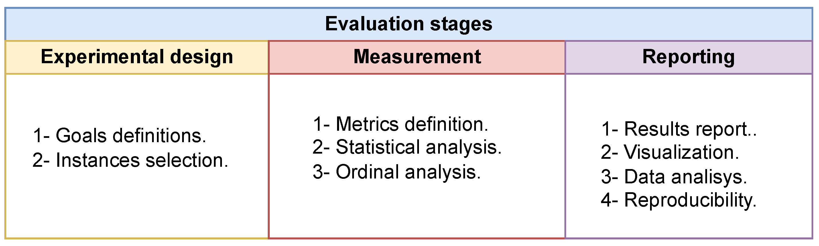
Article

Dynamic Population on Bio-Inspired Algorithms Using Machine Learning for Global Optimization

1
Escuela de Ingeniería Informática, Pontificia Universidad Católica de Valparaíso, Valparaíso 2362807, Chile
2
Departamento de Tecnologías de Información y Comunicación, Universidad de Valparaíso, Valparaíso 2361864, Chile
3
Escuela de Ingeniería Informática, Universidad de Valparaíso, Valparaíso 2362905, Chile
*
Authors to whom correspondence should be addressed.
Biomimetics 2024, 9(1), 7; https://doi.org/10.3390/biomimetics9010007
Submission received: 15 November 2023 / Revised: 20 December 2023 / Accepted: 21 December 2023 / Published: 25 December 2023
(This article belongs to the Special Issue Bioinspired Algorithms)

Abstract

:
In the optimization field, the ability to efficiently tackle complex and high-dimensional problems remains a persistent challenge. Metaheuristic algorithms, with a particular emphasis on their autonomous variants, are emerging as promising tools to overcome this challenge. The term “autonomous” refers to these variants’ ability to dynamically adjust certain parameters based on their own outcomes, without external intervention. The objective is to leverage the advantages and characteristics of an unsupervised machine learning clustering technique to configure the population parameter with autonomous behavior, and emphasize how we incorporate the characteristics of search space clustering to enhance the intensification and diversification of the metaheuristic. This allows dynamic adjustments based on its own outcomes, whether by increasing or decreasing the population in response to the need for diversification or intensification of solutions. In this manner, it aims to imbue the metaheuristic with features for a broader search of solutions that can yield superior results. This study provides an in-depth examination of autonomous metaheuristic algorithms, including Autonomous Particle Swarm Optimization, Autonomous Cuckoo Search Algorithm, and Autonomous Bat Algorithm. We submit these algorithms to a thorough evaluation against their original counterparts using high-density functions from the well-known CEC LSGO benchmark suite. Quantitative results revealed performance enhancements in the autonomous versions, with Autonomous Particle Swarm Optimization consistently outperforming its peers in achieving optimal minimum values. Autonomous Cuckoo Search Algorithm and Autonomous Bat Algorithm also demonstrated noteworthy advancements over their traditional counterparts. A salient feature of these algorithms is the continuous nature of their population, which significantly bolsters their capability to navigate complex and high-dimensional search spaces. However, like all methodologies, there were challenges in ensuring consistent performance across all test scenarios. The intrinsic adaptability and autonomous decision making embedded within these algorithms herald a new era of optimization tools suited for complex real-world challenges. In sum, this research accentuates the potential of autonomous metaheuristics in the optimization arena, laying the groundwork for their expanded application across diverse challenges and domains. We recommend further explorations and adaptations of these autonomous algorithms to fully harness their potential.

1. Introduction

In operation research fields, the role of optimization algorithms is undeniably pivotal. As the complexities of problems across various domains burgeon, so does the necessity for sophisticated optimization strategies [1,2]. Metaheuristics, with their inherent capacity to explore vast solution spaces, have risen to prominence [3]. Yet, with the increasing dimensionality and intricacy of problems, the traditional static management of solution populations often proves inadequate [4,5].
A significant challenge that modern optimization algorithms face is dynamically managing their populations of solutions [6,7]. Traditional approaches often employ static populations, which, while simpler to implement and manage, frequently fall short in adapting to the evolving nature of complex optimization landscapes [8]. Such static management can lead to premature convergence, where the algorithm becomes stuck in local optima without fully exploring potential solutions [9]. Furthermore, without a dynamic adaptation mechanism, algorithms might not efficiently exploit promising regions or explore lesser-known areas of the solution space. This stagnation not only diminishes the algorithm’s potential to locate the global optimum but also curtails its versatility across varied problem instances [10].
In the modern landscape of optimization, the dynamic management of solution populations has transitioned from being a mere enhancement to an absolute necessity [11,12]. Addressing this critical need, our study sets forth with a meticulously crafted approach that marries the strengths of both metaheuristics and clustering techniques. At the forefront of our strategy are three distinguished optimization metaheuristics: particle swarm optimization (PSO), cuckoo search algorithm (CSA), and bat algorithm (BA). Their selection is predicated on their consistent performance and resilience across diverse optimization challenges. Their legacy of success, coupled with their inherent capabilities of exploration and exploitation, underscores their suitability for our ambitious undertaking [11]. To elevate the potential of these bio-inspired solvers, we incorporate the ability of the Density-Based Spatial Clustering of Applications with Noise (DBSCAN) algorithm, a wide-known clustering methodology by the scientific community [13,14]. DBSCAN’s reputation is anchored in its exceptional ability to discern and classify clusters with varied shapes and densities, an aspect where many clustering paradigms falter [15]. Our proposition leans on this strength of DBSCAN, envisaging a harmonious collaboration that magnifies the dynamism in managing solution populations. This union is anticipated to dynamically manage and categorize populations of continuous solutions, thereby refining the adaptability and efficiency of the metaheuristics. The contribution of our study focuses on applying logic centered on the different clusters provided by DBSCAN. Depending on the characteristics of the solutions in each subset, we will apply an increase or decrease in the population in an autonomous way [16]. This variability in the population will enhance the metaheuristic’s ability to intensify or diversify solutions. To ensure the robustness and validity of our integrated approach, a rigorous and methodical evaluation is paramount. We have, therefore, chosen the harder functions of the CEC LSGO suite [17] as the testing ground for our proposition. These functions, renowned in the optimization community, embody a myriad of challenges, from multi-modality to shifting landscapes, serving as an ideal crucible to truly assess the mettle of our strategy [18,19,20]. the CEC LSGO suite, with its diverse and demanding function set, offers a comprehensive canvas, enabling us to probe the strengths and potential limitations of our approach under varied conditions. Our methodology for this evaluation will be meticulous, encompassing multiple runs, diverse initial conditions, and thorough statistical analyses.
The rest of the manuscript is described as follows: Section 2 presents the related work. Section 3 exposes SWEVOH: Self-adaptive Swarm Evolutionary Hybrid Algorithm. Experimental results are described in Section 4. At the end of the manuscript, conclusions are presented in Section 5.

2. Related Work

Optimization and metaheuristics stand at the forefront of innovative problem-solving across diverse fields, marking an era of significant evolution from traditional approaches to sophisticated strategies empowered by genetic algorithms and deep learning [21,22]. This relentless progression towards precision and efficiency has dramatically expanded the potential for discovering optimal solutions in complex landscapes [23,24,25,26].
Genetic and evolutionary algorithms have seen substantial refinements, with more sophisticated selection and mutation processes specifically tailored to tackle the challenges inherent in optimizing complex, high-dimensional systems [22,24]. This has led to algorithms that not only navigate but also effectively map the increasingly complex solution spaces [23,24,25]. Swarm-based optimization, notably particle swarm and ant colony optimization, has similarly advanced, now boasting enhanced capabilities for identifying global optima and skirting local optima—critical features in dynamic and unpredictable environments [27,28,29,30].
In the realm of metaheuristics with dynamic population management, several studies have addressed diverse optimization challenges. One study delves into an NP-hard multi-period production distribution problem, employing a memetic algorithm with population management to simultaneously handle production and distribution decisions, achieving significant savings compared to two-phase methods [31]. Another investigation focuses on a dynamic prey–predator spatial model, introducing the African buffalo optimization metaheuristic and employing autonomous multi-agents to regulate buffalo populations, achieving a balanced coexistence of prey and predators [32].
Other population-based approaches are explored in a study that designs a hybrid architecture, the Linear Modular Population Balancer, dynamically balancing and controlling population size based on learning components, demonstrating effectiveness across discrete and continuous optimization problems [33]. Feature selection, a challenging problem, is addressed using the Grasshopper Optimization Algorithm (GOA) with Evolutionary Population Dynamics to mitigate convergence and stagnation drawbacks, revealing superior performance on various datasets [34]. the Black Hole Algorithm is introduced as a nature-inspired optimization algorithm for data clustering, and a multi-population version is proposed, exhibiting precise results and high convergence rates on benchmark functions and real datasets [35].
Lastly, the Equilibrium Optimizer, inspired by dynamic mass balance, is enhanced with opposition-based learning, Lévy flight, and evolutionary population dynamics, resulting in EOOBLE, a competitive algorithm for high-dimensional global optimization problems, outperforming other metaheuristic algorithms [36].
Merging machine learning with conventional optimization techniques has catalyzed the creation of adaptive systems that continually learn and improve, endowing them with a level of autonomy that drastically enhances their effectiveness in complex process optimization [24,37]. Reinforcement learning and deep neural networks stand out as transformative tools, honing the search for solutions and propelling forward the frontiers of automation and predictive analytics [37,38,39]. the integration of diverse optimization strategies through hybridization has been a leap forward, yielding robust and efficient solutions [40,41,42]. Such integrative approaches have harnessed the adaptability of metaheuristics with the predictive power of machine learning to produce systems that dynamically adjust their search mechanisms, enhancing problem-solving in real-time. This fusion has not only improved algorithmic efficiency but has also broadened the scope of their application, enabling the tackling of previously elusive problems and adeptly handling the uncertainties and complexities of real-world systems [25,30,43].
The optimization landscape has been further enriched by the development of adaptive algorithms that fluidly transition between global and local search strategies, offering more effective exploration and exploitation of the solution space [3]. These adaptive methodologies have shown great promise in managing the variability and complexity of contemporary systems, finding applications in as diverse fields as logistics, energy system management, and the design of cutting-edge materials [23,24,29,39].
The convergence of optimization and machine learning continues to be a fertile area for research and development, heralding an era of intelligent optimization solutions that are not only faster and more efficient but also capable of adapting to an array of complex challenges [29,44,45]. These solutions are set to redefine the future of decision making and system analysis, providing innovative responses to the dynamic and ever-evolving environments of the modern world [25,30,37,39,43].

3. SWEVOH: Self-Adaptive Swarm Evolutionary Hybrid Algorithm

To adequately depict and elucidate the operation of our proposition, it is imperative to initiate by delineating the working principles of the metaheuristics chosen for our investigation. Consequently, we shall commence by providing detailed descriptions of these methodologies.

3.1. Metaheuristics

In this section, we will show which are the metaheuristics used to implement our working idea, which are their characteristics, their parameters, and a brief description of their behavior through a pseudo-code.

3.1.1. Cuckoo Search Algorithm

Skilled in applying metaheuristics for diverse problem-solving, especially adept at large-scale combinatorial optimization within acceptable timeframes. Note that optimal solutions are not always guaranteed [46].
Nowadays. A full set of all nature-inspired algorithms can be found in [47], one of them is CSA, which has several study cases. CSA [48] is inspired by the obligate brood parasitism of some cuckoo species by laying their eggs in the nests of other bird species. In order to simplify the description of the CSA steps are described below:
  • Each cuckoo lays an egg at a time and drops it into a randomly selected nest.
  • The best nests with high-quality eggs will be carried over to the next generation.
  • The number of available host nests is fixed, and the egg laid by a cuckoo is discovered by the host bird with a probability p a [ 0 , 1 ] . In this case, a new random solution is generated.
Every new generation is determined b Equation (1).
x i d ( t + 1 ) = x i d + α L e v y ( β ) , i { 1 , , m } d { 1 , , n }
where x i d is the element d of the solution vector i at iteration t. x i d ( t + 1 ) is a solution in the iteration t + 1 . α > 0 is the step size which should be related to the scales of the problem of interest, the upper and lower bounds that the problem needs to be determined. Lévy flight is computed by Equation (2):
L e v y u = t β , ( 0 < β < 3 )
Lévy flight involves random walks with infinite variance. Algorithm 1 includes pseudo-code for better understanding.

3.1.2. Bat Algorithm

The bat algorithm is a metaheuristic optimization method based on microbats’ echolocation behavior, introduced by Yang in 2010 [49]. It has found wide application in various fields. the algorithm is inspired by the hunting behavior of bats and operates as follows:
  • Initialization: BA starts with a population of bats, each representing a solution in the search space. Each bat has an initial position.
  • Update: Each iteration involves bats updating positions through random flights and adjusting towards better solutions.
  • Solution Improvement: If a bat finds a better solution, it updates its position. If it discovers a better global solution, the best global solution is also updated.
  • Stopping Criterion: The algorithm iterates until a stopping criterion, like a maximum number of iterations, is met. Our three criteria are described as follows:
    • All bats use echolocation to sense distance, and they also “know” the difference between food/prey and background barriers in some magical way.
    • Bats fly randomly with velocity v i at position x i with a fixed frequency f m i n , varying wavelength λ , and loudness A 0 to search for prey. They can automatically adjust the wavelength (or frequency) of their emitted pulses and adjust the rate of pulse emission r [ 0 , 1 ] , depending on the proximity of their target.
    • Although the loudness can vary in many ways, we assume that the loudness varies from a large (positive) A 0 to a minimum constant value A m i n
Algorithm 1: Pseudocode for Cuckoo Search
Biomimetics 09 00007 i001
In addition, for simplicity, they also use the following approximations: in general, the frequency f in a range [ f m i n , f m a x ] corresponds to a range of wavelengths [ λ m i n , λ m a x ] . In fact, they just vary in frequency while fixed in the wavelength λ and assume f [ 0 , f m a x ] in their implementation. This is because λ and f are related due to the fact that λ f = v is constant.
In simulations, they use virtual bats naturally to define the updated rules of their positions x i and velocities v i in a D-dimensional search space. the new solutions x i t and velocities v i t at time step t are given by:
f i = f m i n + ( f m a x f m i n ) β v i t = v i t 1 + ( x i t x b e s t ) f i x i t = x i t 1 + v i t
where β [ 0 , 1 ] is a random vector drawn from a uniform distribution. Here, x c g B e s t is the current global best location (solution) which is located after comparing all the solutions among all the n bats.
For the local search part, once a solution is selected among the current best solutions, a new solution for each bat is generated locally using a random walk:
x n e w = x o l d + ϵ A t
where ϵ [ 1 , 1 ] is a random number, while A t = A i t is the average loudness of all the bats at this time step.
Furthermore, the loudness A i and the rate r i of pulse emission have to be updated accordingly as the iterations proceed. These formulas are:
A i t + 1 = α A i t
r i t + 1 = r i 0 [ 1 e x p ( γ t ) ]
where α and γ are constants.
Based on these approximations and idealization, the pseudo-code of BA is shown in Algorithm 2.
Algorithm 2: Pseudocode for Bat Algorithm.
Biomimetics 09 00007 i002

3.1.3. Particle Swarm Optimization

PSO is a stochastic optimization method inspired by bird flocks and insect swarms. It has diverse applications including neural network training, function optimization, fuzzy control, and pattern classification [50,51]. Operates as follows:
  • Initialization: PSO begins with a population of particles in a search space. Each particle has an initial position and velocity.
  • Update: In each iteration, each particle adjusts its velocity and position based on rules derived from its personal experience and the global experience of the group.
  • Personal Experience: Each particle maintains a record of its best local position. Velocity V i ( t ) is the velocity of particle i at iteration t and position updates aim to converge towards this best local position X i ( t ) is the position of particle i at iteration t. Those formulas are described as follows:
    v i ( t + 1 ) = w · v i ( t ) + c 1 · r 1 · ( p i ( t ) x i ( t ) ) + c 2 · r 2 · ( g ( t ) x i ( t ) )
    x i ( t + 1 ) = x i ( t ) + v i ( t + 1 )
  • Global Experience: The group of particles maintains a record of the best global position found. Particles also adjust their velocity and position to converge towards this best global position.
  • Stopping Criterion: The algorithm continues to iterate until a stopping criterion is satisfied, such as reaching a maximum number of iterations.
In our particle swarm optimization model, each particle’s movement is defined by several key elements: v i ( t ) represents the velocity of particle i at iteration t, determining its speed and direction. x i ( t ) indicates the position of particle i at iteration t, showing its location in the search space. p i ( t ) is the best position personally found by particle i up to iteration t, while g ( t ) denotes the best global position found by any particle up to iteration t, representing the best overall solution so far. the inertia weight w affects the particle’s momentum and its changes in direction. the acceleration coefficients c 1 and c 2 determine the particle’s movement towards its personal best and the global best positions, respectively. Lastly, r 1 and r 2 are random numbers between 0 and 1 that add an element of randomness to the particle’s path.
To delineate the behavior of this metaheuristic, we present its pseudocode in Algorithm 3.
Algorithm 3: Pseudocode for Particle Swarm Optimization.
Biomimetics 09 00007 i003

3.2. SWEVOH Logic

The goal of this component is to dynamically vary the population of the MH with characteristics that enable it to enhance its search space. This involves intensifying by minimizing the population and diversifying by increasing it.
Expanding on this idea, the population variation is a crucial aspect in optimizing the metaheuristic’s performance. When minimizing the population, the algorithm focuses on intensifying its search, aiming for a more concentrated exploration of promising regions. On the other hand, increasing the population facilitates diversification, allowing the algorithm to explore a broader solution space and potentially discover novel, optimal solutions. This dynamic adjustment of the population size plays a pivotal role in balancing between exploitation and exploration, contributing to the adaptability and effectiveness of the metaheuristic across different problem landscapes.
The SWEVOH component’s operational aspects are clarified by using a standard swarm method as an illustrative case to explain its functioning, parameter setup, and execution logic. the integrated SWEVOH Algorithm takes on the responsibility of dynamically supervising and adapting the bat population in response to solution performance and observed enhancements. Its pivotal role involves the continuous adjustment of the algorithm’s population size and composition throughout the optimization procedure. We incorporate the SWEVOH component at the outset of the iterative cycle for each metaheuristic. This ensures that, when the freedom parameter permits population adjustments, the metaheuristic’s continuity proceeds along its regular course. This is exemplified in Algorithm 4, specifically between lines 5 and 7, where it evaluates the need for the self-adaptive strategy in each iteration. Algorithm 4 is intended solely to illustrate the integration point of the autonomous component within each metaheuristic, positioned at the onset of iterations. This autonomous component dynamically adjusts the population size, aligning with the intensification and diversification criteria inherent to each metaheuristic.   
Algorithm 4: Standard Swarm pseudo code with SWEVOH component.
Biomimetics 09 00007 i004
We introduce a flexibility parameter to regulate when to intervene with metaheuristic parameter values. This ensures the metaheuristic maintains its distinctive behavior. After one hundred unrestricted iterations, the algorithm checks for updates based on improvement percentages compared to predefined thresholds.
improvement _ percentage = past _ best current _ best past _ best × 100
  • If the improvement percentage exceeds the defined acceptance value, the component will take the solutions with the worst results and remove them from the search space according to the logic explained in Section 3.3.
  • If the improvement percentage falls below the accepted threshold, indicating insufficient progress, self-tuning strategies adjust the population.

3.3. Self-Tuning Strategies

The following self-tuning strategies are applied when the improvement percentage is below the accepted threshold:
  • Calculation of Clusters: DBSCAN partitions the population into clusters denoted as C = { C 1 , C 2 , , C k } . For the separation of solutions, DBSCAN considers each solution vector X n as an element for processing, where n is the current population size. To calculate the distance between solutions, DBSCAN performs element-wise distance calculations hamming distance. Once DBSCAN performs the clustering of solutions, the average of each obtained cluster is calculated. The average fitness of each cluster A V G C i is computed as:
    A V G C i = 1 | C i | x C i Fitness ( x )
    Here, | C i | denotes the number of solutions in cluster C i and Fitness ( x ) represents the evaluation of the solution x in the objective function. Each cluster is assessed based on the average fitness it contains to determine the sector where population size adjustments should be applied. The least-performing solutions from the worst fitness cluster ( C worst ) will be employed to reduce the population size, while the best solutions ( C best ) from the best fitness cluster will be utilized to increase the population size.
    The use of fitness-based cluster evaluations guides precise population modifications, ensuring a balanced and effective population management strategy.
  • Population Variation: In the process of expanding the population within defined constraints, a meticulous verification ensures that the addition of new solutions aligns with the set maximum population size N Population _ max . Selecting I n c r e m e n t _ s o l u t i o n s _ x _ c l u s t e r superior solutions from the cluster boasting the highest fitness ( C best ) initiates the generation phase. The quantity of newly generated solutions is regulated by the parameter I n c r e m e n t _ s o l u t i o n s _ x _ c l u s t e r , maintaining a controlled expansion. Crucially, the logic governing the creation of these solutions remains faithful to the core principles intrinsic to each respective metaheuristic. In the scenario where it is feasible to reduce the population, ensuring it does not fall below the specified parameter N Population _ min , a procedure analogous to the one described earlier is implemented. This involves considering the I n c r e m e n t _ s o l u t i o n s _ x _ c l u s t e r parameter negatively, applied to the cluster with the worst fitness performance ( C worst ).
  • Replacement of solution: If the calculated clusters exhibit an average of solutions within an acceptable parameter range ( D i f f _ c l u s t e r _ % _ a c c e p t e d ), it suggests that all solutions are converging to a local stagnation point. To address this, we replace half of the solutions in each underperforming cluster with new random solutions generated using the functions specific to each metaheuristic.
The SWEVOH component dynamically manages the metaheuristic population by monitoring the algorithm’s performance evolution. The population is kept stable if significant enhancements are noted. However, if the improvements are deemed insufficient, the function deploys self-tuning strategies to alter the population’s size and composition, all the while considering the clustering structure of the solutions. This adaptive method enables the algorithm to effectively navigate the search space and adjust to the continuously changing optimization landscapes.
Finally, it is crucial reinforcing that the computational complexity of the metaheuristics employed in this study is generally O ( k n ) , where n represents the dimension of the problem and k stands for the constant combining the total number of iterations or generations with the population size. This denotes the cumulative number of objective function evaluations conducted throughout the execution of the algorithm. Additionally, at specific intervals, the complexity of the DBSCAN algorithm, typically O ( n log n ) , must be considered. This is due to the potential necessity for comparing all pairs of points within the dataset. Incorporating DBSCAN’s complexity into the metaheuristics framework undeniably elevates the overall computational cost. However, this increase is justifiable given the enhanced outcomes achieved. Furthermore, it is important to note the ever-increasing accessibility of computing power, driven by continuous technological advancements, which helps mitigate the impact of this added complexity.

4. Experimental Results

To evaluate the performance of our proposal, we test the CEC LSGO functions, comparing the original metaheuristics with standard configurations, versus the SWEVOH.

4.1. Methodology

To adequately evaluate the performance of metaheuristics, a performance analysis is required [52]. For this work, we compare the supplied best solution of the SWEVOH to the best-known result of the benchmark retrieved from [17]. Figure 1 depicts the procedures involved in doing a thorough examination of the enhanced metaheuristic. We create objectives and recommendations for the experimental design to show that the proposed approach is a viable alternative for determining metaheuristic parameters. Then, as a vital indicator for assessing future results, we evaluate the best value. We use ordinal analysis and statistical testing to evaluate whether a strategy is significantly better in this circumstance. Lastly, we detail the hardware and software aspects that were used to replicate computational experiments, and we present all of the results in tables and graphs.
As a result, we conduct a contrast statistical test for each case, using the Kolmogorov–Smirnov–Lilliefors process [53] to measure sample autonomy and the Mann–Whitney–Wilcoxon [54] test to statistically evaluate the data. In Figure 2, we describe and determine the organization.
The Kolmogorov–Smirnov–Lilliefors test allows us to assess sample independence by calculating the Z M I N or Z M A X (depending on whether the task is minimization or maximization) obtained from each instance’s 31 executions.
All functions within the CEC LSGO reach their maximum efficiency at 0; hence, in order to discern the most favorable values obtained, it is essential to ascertain those that approach zero or are in close proximity to this value. The best obtained values can be visualized in bold.

4.2. CEC LSGO Function Results

Infrastructure: Python 3.10 was used to implement SWEVOH. The computer has the common attributes: MacOS with a 2.7 GHz Intel Core i7 CPU and 16 GB of RAM.
Setup variables: The configuration for our suggested approach is shown in Table 1, Table 2, Table 3 and Table 4.
Fifteen functions were considered, each of which was run 31 times; the results are presented in Table 5, Table 6 and Table 7.
The algorithms are ranked in order of Z m i n achieved. The instances that obtained Z m i n are also displayed. As can be seen in the results of the algorithms that solved CEC LSGO function, we compare the distribution of the samples of each instance using a violin plot, which allows us to observe the entire distribution of the data. We provide and discuss the most difficult instances of each group to create a resume of all the instances below:
The information is organized as follows: MIN: the minimum value reached; MAX: the maximum value reached; MEAN: the average value.
The first method was the standard cuckoo search algorithm with various settings, and the second was SACSDBSCAN, as previously indicated.
As depicted in Table 5, the comparative analysis showcases the performance disparities between the Original PSO Algorithm and the Autonomous PSO Algorithm across various high-density functions from the CEC. The table delineates the minimum, maximum, and mean values for both algorithmic versions concerning these functions. Notably, upon examination, a trend emerges wherein the Autonomous PSO Algorithm demonstrates superior performance in terms of minimum values across the majority of functions. This trend suggests an enhanced search capability exhibited by the Autonomous PSO Algorithm compared to the Original PSO, signifying its efficacy in exploring the solution space to discover more optimal or near-optimal solutions, particularly evident in its consistently lower minimum values across diverse functions.
In the distribution of the data in the functions 10 to 15 (Figure 3, Figure 4, Figure 5, Figure 6, Figure 7 and Figure 8), as we can observe the behavior of our proposal aligns with the hybrid logic as initially envisaged. This allows for a broader search space coverage, concentrating the highest density of optimal values near the vicinity of the known minimum.
Table 6 offers a comprehensive comparison between two variants of the Cuckoo Search Algorithm (CSA): the Original Cuckoo Search Algorithm and the Autonomous Cuckoo Search Algorithm across multiple high-density functions derived from the CEC dataset. The table presents essential statistical values including minimum, maximum, and mean values obtained for each function under both algorithmic versions.
Notably, upon analysis, it becomes evident that the Autonomous Cuckoo Search Algorithm consistently outperforms the Original Cuckoo Search Algorithm, particularly in achieving superior minimum values across a majority of the evaluated functions. This observed trend signifies a noteworthy improvement in the efficiency and efficacy of the Autonomous Cuckoo Search Algorithm compared to its original counterpart. The ability of the Autonomous variant to consistently yield better minimum values suggests a heightened capability to explore and discover more optimal or near-optimal solutions within the solution space for a diverse set of functions, showcasing its enhanced algorithmic effectiveness and potential for improved performance in optimization tasks.
Similar to the images observed in the PSO algorithm, the distribution of our proposal remains consistent in its shape and behavior. The images (Figure 9, Figure 10, Figure 11, Figure 12, Figure 13 and Figure 14) demonstrate that for the indicated functions, the distribution of the 31 executions enables a more effective exploration of the search space, facilitating the discovery of solutions that lead to improved optimal values.
Table 7 presents a detailed comparison between two variations of the Bat Algorithm (BA): the Original Bat Algorithm and the Autonomous Bat Algorithm, denoted as SWEVOH-BA. This comparison encompasses a range of high-density functions from the CEC dataset, illustrating essential statistical values including minimum, maximum, and mean values for each function under both algorithmic versions.
Upon analysis, a notable trend emerges: the Autonomous Bat Algorithm consistently demonstrates notably superior minimum values when compared to the Original Bat Algorithm across various functions. This significant difference in minimum values implies a tangible enhancement in the performance and optimization capabilities of the Autonomous Bat Algorithm. Specifically, the consistently lower minimum values achieved by the Autonomous variant suggest its heightened efficiency in exploring the solution space and locating more optimal or near-optimal solutions across diverse functions.
This observed improvement in achieving better minimum values signifies the efficacy and potential superiority of the Autonomous Bat Algorithm in optimizing and solving optimization problems, showcasing its enhanced performance compared to the Original Bat Algorithm.
Similar to the images observed in the BA algorithm, the distribution of our proposal remains consistent in its shape and behavior. Images (Figure 15, Figure 16, Figure 17, Figure 18, Figure 19 and Figure 20), demonstrate that for the indicated functions, the distribution of the 31 executions enables a more effective exploration of the search space, facilitating the discovery of solutions that lead to improved optimal values.
Overall, the results indicate that autonomous algorithms enhance performance compared to their original counterparts in most high-density functions from the CEC. Specifically, the Autonomous PSO Algorithm achieves better minimum results in most functions. The Autonomous Cuckoo Search Algorithm also outperforms the Original Cuckoo Search in terms of minimum values in multiple functions. Lastly, the Autonomous Bat Algorithm demonstrates superior performance compared to the Original Bat Algorithm in terms of minimum values in several functions. Furthermore, Figure 21 below shows how the population dynamically adjusts according to what is described in the Section 3.3, which is directly related to what is observed in Figure 22 that shows how the metaheuristic works with an expected convergence, which has caused the number of the population to increase. Another example of what was described above can be seen in the Figure 23 and Figure 24 that belongs to function 9 in Table 8.

4.3. Statistical Test

We present the following hypotheses to assess independence.
-
H 0 : states that Z m i n / Z m a x follows a normal distribution.
-
H 1 : states the opposite.
The test resulted in a p-value below 0.05, indicating that H 0 cannot be assumed. With independent samples and a non-normal distribution, the central limit theorem does not apply. Therefore, we employ the non-parametric Mann–Whitney–Wilcoxon test to assess heterogeneity in the results of the most challenging instances. We propose the following hypotheses:
-
H 0 : CSA is better than SACSDBSCAN
-
H 1 : states the opposite.
The statistical contrast test ultimately determines which technique is significantly superior.
The Wilcoxon signed rank test was used to compare LSGO CEC function on the algorithms techniques. Smaller values than 0.05 define that H 0 cannot be assumed because the significance level is also set to 0.05 .
To conduct the test run that supports the study, we use a method from the PISA system. We specify all data distributions (each in a file and each data in a line) in this procedure, and the algorithm returns a p-value for the hypotheses.
The following tables show the result of the Mann–Whitney–Wilcoxon test. To understand them, it is necessary to know the following acronyms:
  • SWS = Statistically without significance.
SWEVOH-PSO vs. PSO—p-value
The p-values for each function’s results are presented in Table 9, Table 10, Table 11, Table 12, Table 13, Table 14, Table 15, Table 16, Table 17, Table 18, Table 19, Table 20, Table 21, Table 22 and Table 23. In 8 of 15 cases, the reported p-values are less than 0.05, indicating a statistically significant difference between SWEVOH-PSO and PSO for evaluated functions. Hence, we can conclude that SWEVOH-PSO is statistically superior to PSO in those evaluated functions in this study.
SWEVOH-CSA vs. CSA—p-value.
The p-values for each function’s results are presented in Table 24, Table 25, Table 26, Table 27, Table 28, Table 29, Table 30, Table 31, Table 32, Table 33, Table 34, Table 35, Table 36, Table 37 and Table 38. In 7 of 15 cases, as mentioned above, t. he p-values reported are less than 0.05, and SWS suggests that they have no statistical significance. So, with this knowledge, in each instance mentioned, we can see the SWEVOH-CSA algorithm was better than the original CSA. In four out of the remaining eight cases, none can demonstrate significant superiority over the other.
If we focus on the instances where our proposal improves the result obtained in comparison to the original CSA, we can infer that the solutions achieved are distributed in a centered way on their optimal value, which reflects that the behavior of this algorithm is according to the SWEVOH behavior. This is reflected in the violin graphs in Figure 9, Figure 10 and Figure 12.
SWEVOH-BA vs. BA—p-value.
The p-values for each function’s results are presented in Table 39, Table 40, Table 41, Table 42, Table 43, Table 44, Table 45, Table 46, Table 47, Table 48, Table 49, Table 50, Table 51, Table 52 and Table 53. In 8 of 15 scenarios, the p-values reported are less than 0.05, and 7 of the remaining cases are both SWS, which suggests that they have no statistical significance. So, with this knowledge, in each instance mentioned, we can see the SWEVOH-BA algorithm was better than the original BA.

5. Conclusions

In this study, we have proposed an integrated approach that combines metaheuristics and clustering techniques to address the challenge of dynamically managing solution populations in optimization algorithms. Our approach is based on three optimization metaheuristics: Particle Swarm Optimization (PSO), Cuckoo Search Algorithm (CSA), and Bat Algorithm (BA), which have consistently demonstrated good performance across a variety of optimization challenges.
Moreover, the DBSCAN clustering algorithm has been integrated to enhance the capability for dynamic management and categorization of solution populations. This incorporation facilitates the adjustment of solution numbers within the metaheuristic dynamically, increasing solutions when diversification is needed or reducing them during intensification scenarios.
The evaluation of our approach was conducted using the complex functions from the widely recognized CEC LSGO test suite in the optimization community. Our results demonstrate that our integrated approach achieves significantly better performance compared to traditional approaches of static population management. This is attributed to our approach’s capacity to dynamically adapt to changes in the optimization landscape and explore promising regions within the solution space.
Furthermore, we performed a comprehensive statistical analysis to assess the significance of the obtained results. We employed Kolmogorov–Smirnov–Lilliefors and Mann–Whitney–Wilcoxon tests to evaluate sample independence and conduct statistical comparisons, respectively. These analyses allowed us to conclusively demonstrate the superiority of our integrated approach in terms of performance.
It is essential to note that the replicability of our experiments was ensured by using standard hardware and software widely accepted in the optimization community. All obtained results are presented clearly and concisely in tables and graphs to facilitate their comprehension and analysis.
In summary, our integrated approach of metaheuristics and clustering proves to be a viable and effective alternative for the dynamic management of solution populations in optimization algorithms. Our results, supported by a comprehensive statistical analysis, substantiate that our approach significantly outperforms traditional approaches to static population management. This is attributed to our approach’s ability to dynamically adapt to changes in the optimization landscape and explore promising regions within the solution space.
Additionally, it is noteworthy that our experiments were replicable using standard hardware and software within the optimization community. All results obtained are presented clearly and concisely in tables and graphs, making them easily understandable and analyzable.
As part of our future endeavors, we aim to explore approaches to enhance the precision of solution narrowing, preserving the metaheuristic’s proficiency in discovering superior solutions.
In conclusion, our integrated approach offers an effective and promising solution to address the challenge of dynamically managing solution populations in optimization algorithms. The results obtained provide evidence for the superiority of our approach and lay the foundation for future research in this field.

Author Contributions

Formal analysis, N.C., R.S. and B.C.; Investigation, N.C., R.S., B.C., S.V., and R.O.; Methodology, R.S., R.O. and S.V.; Resources, R.S. and B.C.; Software, N.C., S.V. and R.O.; Validation, B.C. and S.V.; Writing—original draft, N.C., S.V. and R.O.; Writing—review and editing, N.C., R.S., B.C., S.V., R.O. and E.C. All the authors of this paper hold responsibility for every part of this manuscript. All authors have read and agreed to the published version of the manuscript.

Funding

Broderick Crawford is supported by grant ANID/FONDECYT/REGULAR/1210810. Rodrigo Olivares is supported by grant ANID/FONDECYT/INICIACION/11231016. Nicolás Caselli is supported by grant INF-PUCV 2019-2023.

Institutional Review Board Statement

Not applicable.

Data Availability Statement

Data is available on http://doi.org/10.6084/m9.figshare.24899883 (accessed on 19 December 2023).

Conflicts of Interest

The authors declare no conflicts of interest. The founding sponsors had no role in the design of the study; in the collection, analyses, or interpretation of data; in the writing of the manuscript; or in the decision to publish the results.

References

  1. Valdivia, S.; Soto, R.; Crawford, B.; Caselli, N.; Paredes, F.; Castro, C.; Olivares, R. Clustering-Based Binarization Methods Applied to the Crow Search Algorithm for 0/1 Combinatorial Problems. Mathematics 2020, 8, 1070. [Google Scholar] [CrossRef]
  2. Caselli, N.; Soto, R.; Crawford, B.; Valdivia, S.; Olivares, R. A Self-Adaptive Cuckoo Search Algorithm Using a Machine Learning Technique. Mathematics 2021, 9, 1840. [Google Scholar] [CrossRef]
  3. Hussain, K.; Salleh, M.N.M.; Cheng, S.; Shi, Y. On the exploration and exploitation in popular swarm-based metaheuristic algorithms. Neural Comput. Appl. 2019, 31, 7665–7683. [Google Scholar] [CrossRef]
  4. Morales-Castaneda, B.; Zaldivar, D.; Cuevas, E.; Fausto, F.; Rodriguez, A. A better balance in metaheuristic algorithms: Does it exist? Swarm Evol. Comput. 2020, 54, 100671. [Google Scholar] [CrossRef]
  5. Xu, J.; Xu, L. Optimal Stochastic Process Optimizer: A New Metaheuristic Algorithm with Adaptive Exploration-Exploitation Property. IEEE Access 2021, 9, 108640–108664. [Google Scholar] [CrossRef]
  6. Wang, M.; Li, B.; Zhang, G.; Yao, X. Population Evolvability: Dynamic Fitness Landscape Analysis for Population-Based Metaheuristic Algorithms. IEEE Trans. Evol. Comput. 2018, 22, 550–563. [Google Scholar] [CrossRef]
  7. Vincent, B.; Duhamel, C.; Ren, L.; Tchernev, N. A population-based metaheuristic for the capacitated lot-sizing problem with unrelated parallel machines. Int. J. Prod. Res. 2020, 58, 6689–6706. [Google Scholar] [CrossRef]
  8. Creput, J.C.; Hajjam, A.; Koukam, A.; Kuhn, O. Self-organizing maps in population based metaheuristic to the dynamic vehicle routing problem. J. Comb. Optim. 2012, 24, 437–458. [Google Scholar] [CrossRef]
  9. Yeoh, J.M.; Caraffini, F.; Homapour, E.; Santucci, V.; Milani, A. A Clustering System for Dynamic Data Streams Based on Metaheuristic Optimisation. Mathematics 2019, 7, 1229. [Google Scholar] [CrossRef]
  10. Abd Elaziz, M.; Yousri, D.; Mirjalili, S. A hybrid Harris hawks-moth-flame optimization algorithm including fractional-order chaos maps and evolutionary population dynamics. Adv. Eng. Soft. 2021, 154, 102973. [Google Scholar] [CrossRef]
  11. Abed-alguni, B.H.; Alkhateeb, F. Novel Selection Schemes for Cuckoo Search. Arab. J. Sci. Eng. 2017, 42, 3635–3654. [Google Scholar] [CrossRef]
  12. Yang, X.S.; Deb, S.; Fong, S. Metaheuristic Algorithms: Optimal Balance of Intensification and Diversification. Appl. Math. Inf. Sci. 2014, 8, 977–983. [Google Scholar] [CrossRef]
  13. Bhattacharjee, P.; Mitra, P. A survey of density based clustering algorithms. Front. Comput. Sci. 2021, 15, 151308. [Google Scholar] [CrossRef]
  14. Zhang, X.; Liu, H.; Zhang, X. Novel density-based and hierarchical density-based clustering algorithms for uncertain data. Neural Netw. 2017, 93, 240–255. [Google Scholar] [CrossRef] [PubMed]
  15. Al-Asadi, S.A.; Al-Mamory, S.O. An Improved BAT Algorithm Using Density-Based Clustering. Intel. Artif.-Iberoam. J. Artif. Intell. 2023, 26, 102–123. [Google Scholar] [CrossRef]
  16. Hamadi, Y.; Monfroy, E.; Saubion, F. (Eds.) Autonomous Search; Springer: Berlin/Heidelberg, Germany, 2012. [Google Scholar] [CrossRef]
  17. Li, X.; Tang, K.; Omidvar, M.N.; Yang, Z.; Qin, K. Benchmark Functions for the CEC’2013 Special Session and Competition on Large-Scale Global Optimization. 2013. Available online: https://www.tflsgo.org/assets/cec2018/cec2013-lsgo-benchmark-tech-report.pdf (accessed on 23 December 2023).
  18. Vakhnin, A.; Sopov, E. A Novel Self-Adaptive Cooperative Coevolution Algorithm for Solving Continuous Large-Scale Global Optimization Problems. Algorithms 2022, 15, 451. [Google Scholar] [CrossRef]
  19. Vakhnin, A.; Sopov, E.; Semenkin, E. On Improving Adaptive Problem Decomposition Using Differential Evolution for Large-Scale Optimization Problems. Mathematics 2022, 10, 4297. [Google Scholar] [CrossRef]
  20. Zhang, W.; Lan, Y. A Novel Memetic Algorithm Based on Multiparent Evolution and Adaptive Local Search for Large-Scale Global Optimization. Comput. Intell. Neurosci. 2022, 2022, 3558385. [Google Scholar] [CrossRef]
  21. Zu, Y. Deep learning parallel computing and evaluation for embedded system clustering architecture processor. Des. Autom. Embed. Syst. 2020, 24, 145–159. [Google Scholar] [CrossRef]
  22. Benitez-Hidalgo, A.; Nebro, A.J.; Garcia-Nieto, J.; Oregi, I.; Del Ser, J. jMetalPy: A Python framework for multi-objective optimization with metaheuristics. Swarm Evol. Comput. 2019, 51, 100598. [Google Scholar] [CrossRef]
  23. Nelson, N.G.; Muñoz-Carpena, R.; Phlips, E. Parameter uncertainty drives important incongruities between simulated chlorophylla and phytoplankton functional group dynamics in a mechanistic management model. Environ. Model. Softw. 2020, 129, 104708. [Google Scholar] [CrossRef]
  24. Tang, X.; Machimura, T.; Li, J.; Liu, W.; Hong, H. A novel optimized repeatedly random undersampling for selecting negative samples: A case study in an SVM-based forest fire susceptibility assessment. J. Environ. Manag. 2020, 271, 111014. [Google Scholar] [CrossRef] [PubMed]
  25. Taylor, T.R.; Chao, C.T.; Chiou, J.S. Novel Deep Level Image State Ensemble Enhancement Method for M87 Imaging. Appl. Sci. 2020, 10, 3952. [Google Scholar] [CrossRef]
  26. Camacho-Vallejo, J.F.; Corpus, C.; Villegas, J.G. Metaheuristics for bilevel optimization: A comprehensive review. Comput. Oper. Res. 2024, 161, 106410. [Google Scholar] [CrossRef]
  27. Cao, S.; Dang, N.; Ren, Z.; Zhang, J.; Deguchi, Y. Lagrangian analysis on routes to lift enhancement of airfoil by synthetic jet and their relationships with jet parameters. Aerosp. Sci. Technol. 2020, 104, 105947. [Google Scholar] [CrossRef]
  28. Banerjee, S. To capture the research landscape of lecture capture in university education. Comput. Educ. 2021, 160, 104032. [Google Scholar] [CrossRef] [PubMed]
  29. Golestani, M.; Mobayen, S.; HosseinNia, S.H.; Shamaghdari, S. An LMI Approach to Nonlinear State-Feedback Stability of Uncertain Time-Delay Systems in the Presence of Lipschitzian Nonlinearities. Symmetry 2020, 12, 1883. [Google Scholar] [CrossRef]
  30. Majcen Rosker, Z.; Vodicar, M. Sport-Specific Habitual Adaptations in Neck Kinesthetic Functions Are Related to Balance Controlling Mechanisms. Appl. Sci. 2020, 10, 8965. [Google Scholar] [CrossRef]
  31. Boudia, M.; Prins, C. A memetic algorithm with dynamic population management for an integrated production-distribution problem. Eur. J. Oper. Res. 2009, 195, 703–715. [Google Scholar] [CrossRef]
  32. Almonacid, B.; Aspee, F.; Yimes, F. Autonomous Population Regulation Using a Multi-Agent System in a Prey-Predator Model That Integrates Cellular Automata and the African Buffalo Optimization Metaheuristic. Algorithms 2019, 12, 59. [Google Scholar] [CrossRef]
  33. Vega, E.; Soto, R.; Contreras, P.; Crawford, B.; Pena, J.; Castro, C. Combining a Population-Based Approach with Multiple Linear Models for Continuous and Discrete Optimization Problems. Mathematics 2022, 10, 2920. [Google Scholar] [CrossRef]
  34. Mafarja, M.; Aljarah, I.; Heidari, A.A.; Hammouri, A.I.; Faris, H.; Al-Zoubi, A.M.; Mirjalili, S. Evolutionary Population Dynamics and Grasshopper Optimization approaches for feature selection problems. Knowl.-Based Syst. 2018, 145, 25–45. [Google Scholar] [CrossRef]
  35. Salih, S.A.; Alsewari, A.; Wahab, H.a.S.; Mohammed, M.K.A.; Rashid, T.; Das, D.; Basurra, S. Multi-population Black Hole Algorithm for the problem of data clustering. PLoS ONE 2023, 18, e0288044. [Google Scholar] [CrossRef] [PubMed]
  36. Zhong, C.; Li, G.; Meng, Z.; He, W. Opposition-based learning equilibrium optimizer with Levy flight and evolutionary population dynamics for high-dimensional global optimization problems. Expert Syst. Appl. 2023, 215, 119303. [Google Scholar] [CrossRef]
  37. Liang, B.; Wu, D.; Wu, P.; Su, Y. An energy-aware resource deployment algorithm for cloud data centers based on dynamic hybrid machine learning. Knowl.-Based Syst. 2021, 222, 107020. [Google Scholar] [CrossRef]
  38. Holte, A.J.; Ferraro, F.R. Anxious, bored, and (maybe) missing out: Evaluation of anxiety attachment, boredom proneness, and fear of missing out (FoMO). Comput. Hum. Behav. 2020, 112, 106465. [Google Scholar] [CrossRef]
  39. Zhang, B.; Xu, L.; Zhang, J. Balancing and sequencing problem of mixed-model U-shaped robotic assembly line: Mathematical model and dragonfly algorithm based approach. Appl. Soft Comput. 2021, 98, 106739. [Google Scholar] [CrossRef]
  40. Alkabbani, H.; Ahmadian, A.; Zhu, Q.; Elkamel, A. Machine Learning and Metaheuristic Methods for Renewable Power Forecasting: A Recent Review. Front. Chem. Eng. 2021, 3, 665415. [Google Scholar] [CrossRef]
  41. Antonio, B.R.; Dania, T.V. Machine learning based metaheuristic hybrids for S-box optimization. J. Ambient Intell. Hum. Comput. 2020, 11, 5139–5152. [Google Scholar]
  42. Akhter, M.N.; Mekhilef, S.; Mokhlis, H.; Shah, N.M. Review on forecasting of photovoltaic power generation based on machine learning and metaheuristic techniques. IET Renew. Power Gener. 2019, 13, 1009–1023. [Google Scholar] [CrossRef]
  43. Dwivedi, Y.K.; Hughes, D.L.; Coombs, C.; Constantiou, I.; Duan, Y.; Edwards, J.S.; Gupta, B.; Lal, B.; Misra, S.; Prashant, P.; et al. Impact of COVID-19 pandemic on information management research and practice: Transforming education, work and life. Int. J. Inf. Manag. 2020, 55, 102211. [Google Scholar] [CrossRef]
  44. Thimabut, N.; Yotnuengnit, P.; Charoenlimprasert, J.; Sillapachai, T.; Hirano, S.; Saitoh, E.; Piravej, K. Effects of the Robot-Assisted Gait Training Device Plus Physiotherapy in Improving Ambulatory Functions in Patients with Subacute Stroke with Hemiplegia: An Assessor-Blinded, Randomized Controlled Trial. Arch. Phys. Med. Rehabil. 2022, 103, 843–850. [Google Scholar] [CrossRef] [PubMed]
  45. de Sousa, W., Jr.; Montevechi, J.A.B.; Miranda, R.d.C.; Rocha, F.; Vilela, F.F. Economic Lot-Size Using Machine Learning Parallelism Metaheuristic and Simulation. Int. J. Simul. Model. 2019, 18, 205–216. [Google Scholar] [CrossRef] [PubMed]
  46. Lewis, R. A survey of metaheuristic-based techniques for University Timetabling problems. Spectr. 2008, 30, 167–190. [Google Scholar] [CrossRef]
  47. Tzanetos, A.; Fister, I.; Dounias, G. A comprehensive database of Nature-Inspired Algorithms. Data Brief 2020, 31, 105792. [Google Scholar] [CrossRef]
  48. Yang, X.S.; Deb, S. Cuckoo Search via Levy Flights. In Proceedings of the 2009 World Congress on Nature & Biologically Inspired Computing (NaBIC), Coimbatore, India, 9–11 December 2010. [Google Scholar]
  49. Yang, X.S. A New Metaheuristic Bat-Inspired Algorithm. In Nature Inspired Cooperative Strategies for Optimization (NICSO 2010); González, J.R., Pelta, D.A., Cruz, C., Terrazas, G., Krasnogor, N., Eds.; Springer: Berlin/Heidelberg, Germany, 2010; pp. 65–74. [Google Scholar] [CrossRef]
  50. Engelbrecht, A.P. Fundamentals of Computational Swarm Intelligence; Wiley: Hoboken, NJ, USA, 2005. [Google Scholar]
  51. Poli, R. Analysis of the Publications on the Applications of Particle Swarm Optimisation. J. Artif. Evol. Appl. 2008, 2008, e685175. [Google Scholar] [CrossRef]
  52. Bartz-Beielstein, T.; Preuss, M. Experimental research in evolutionary computation. In Proceedings of the 9th Annual Conference Companion on Genetic and Evolutionary Computation, London, UK, 7–11 July 2007; pp. 3001–3020. [Google Scholar]
  53. Lilliefors, H. On the Kolmogorov-Smirnov Test for Normality with Mean and Variance Unknown. J. Am. Stat. Assoc. 1967, 62, 399–402. [Google Scholar] [CrossRef]
  54. Mann, H.; Donald, W. On a Test of Whether one of Two Random Variables is Stochastically Larger than the Other. Ann. Math. Stat. 1947, 18, 50–60. [Google Scholar] [CrossRef]
Figure 1. Evaluation stages to determine the performance of an metaheuristic.
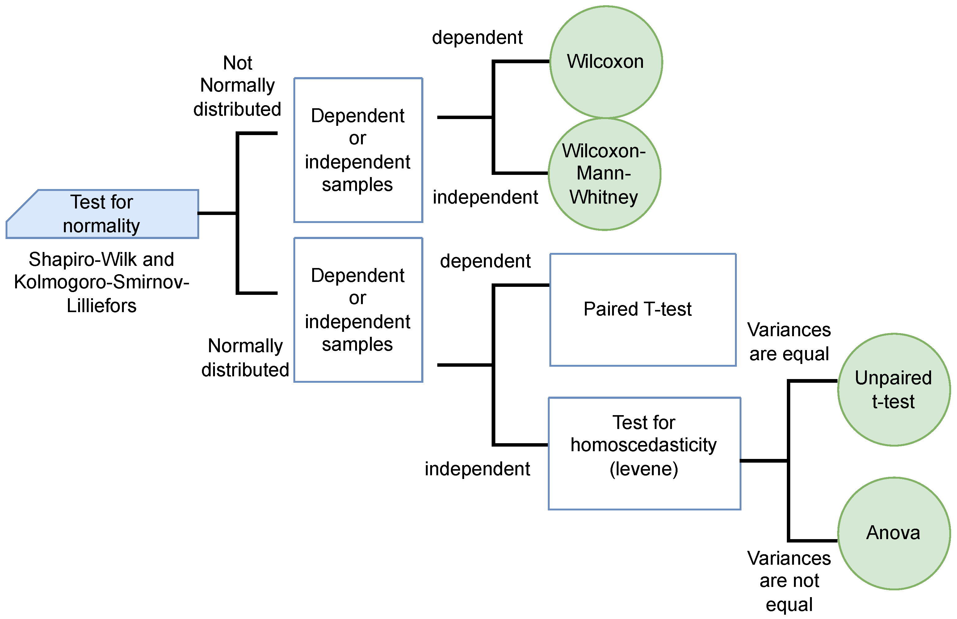
Biomimetics 09 00007 g001
Figure 2. Statistical significance test.
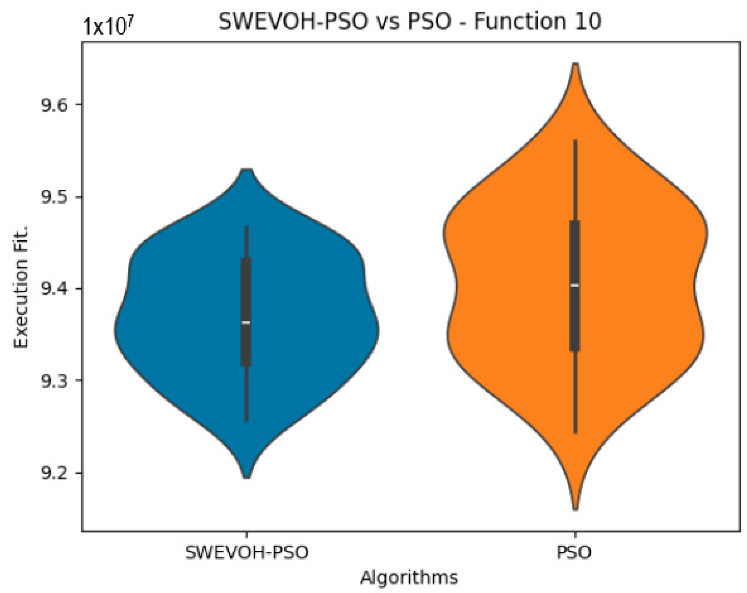
Biomimetics 09 00007 g002
Figure 3. SWEVO-PSO vs. PSO distribution on F10.
Biomimetics 09 00007 g003
Figure 4. SWEVO-PSO vs. PSO distribution on F11.
Biomimetics 09 00007 g004
Figure 5. SWEVO-PSO vs. PSO distribution on F12.
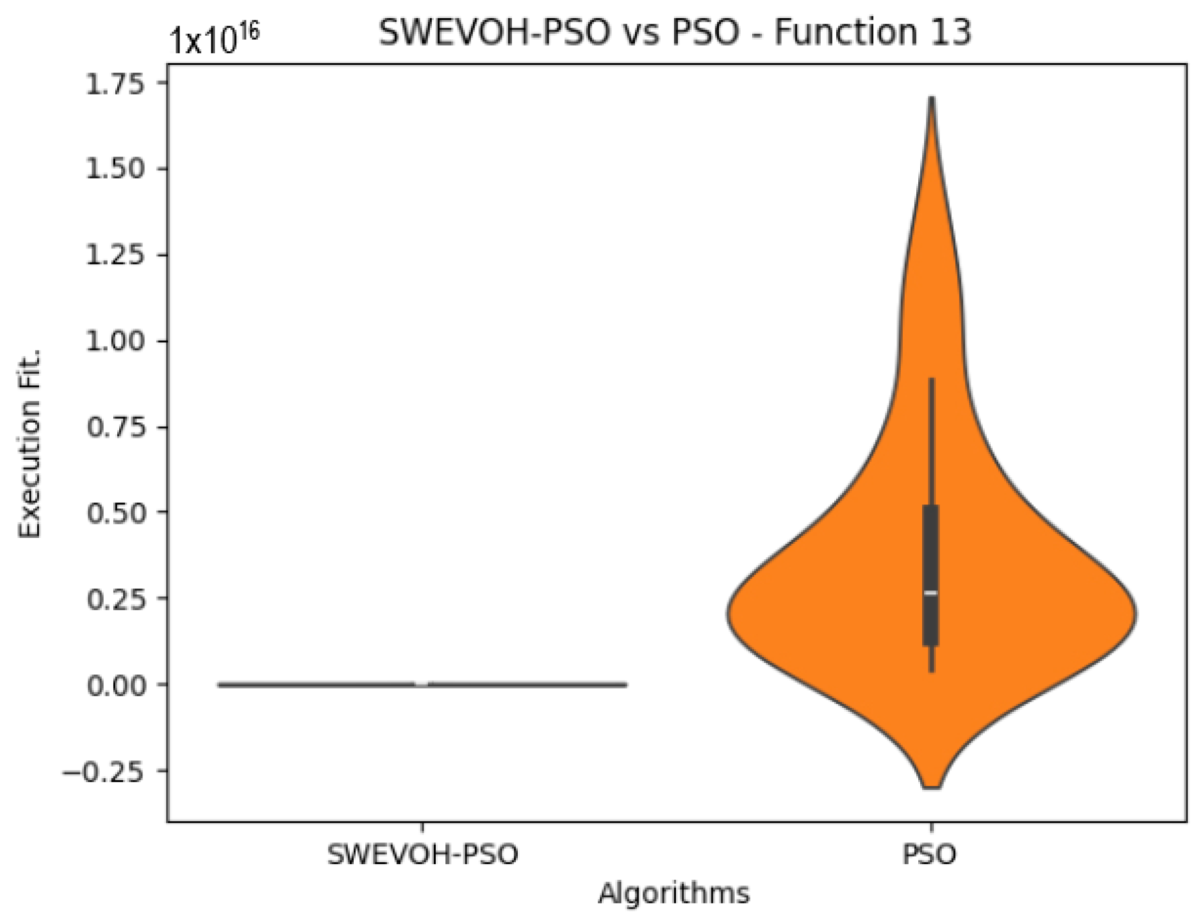
Biomimetics 09 00007 g005
Figure 6. SWEVO-PSO vs. PSO distribution on F13.
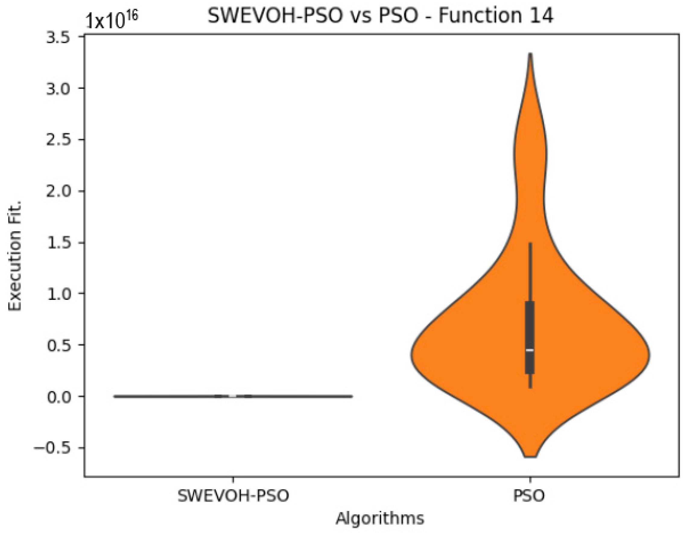
Biomimetics 09 00007 g006
Figure 7. SWEVO-PSO vs. PSO distribution on F14.
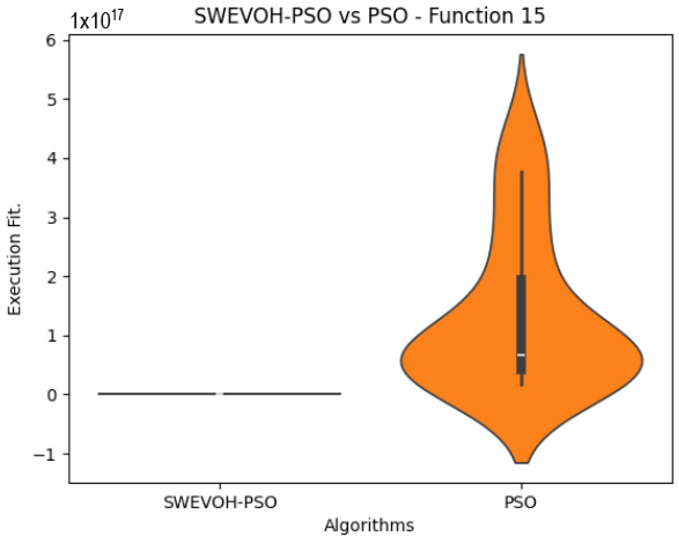
Biomimetics 09 00007 g007
Figure 8. SWEVO-PSO vs. PSO distribution on F15.
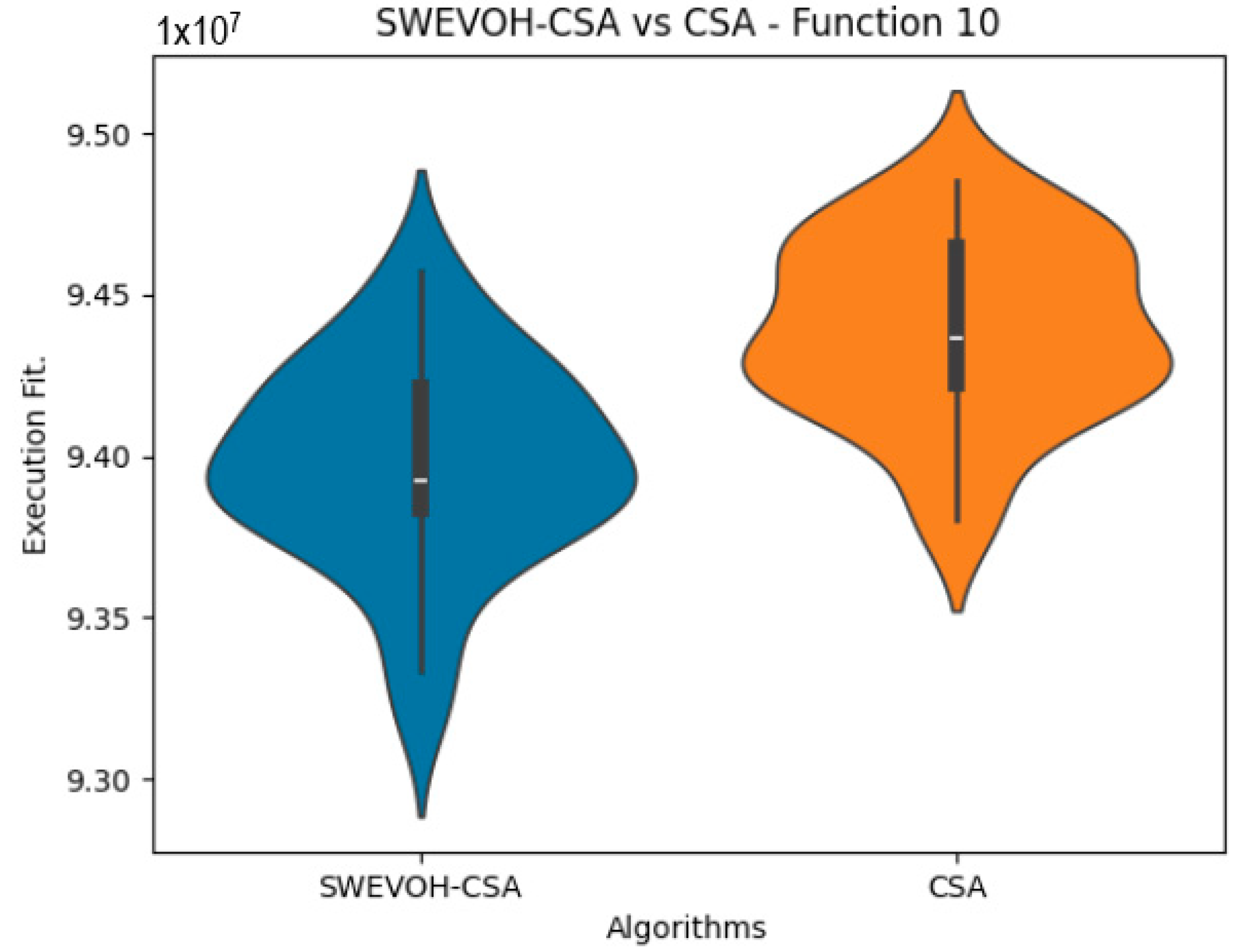
Biomimetics 09 00007 g008
Figure 9. SWEVO-CSA vs. CSA distribution on F10.
Biomimetics 09 00007 g009
Figure 10. SWEVO-CSA vs. CSA distribution on F11.
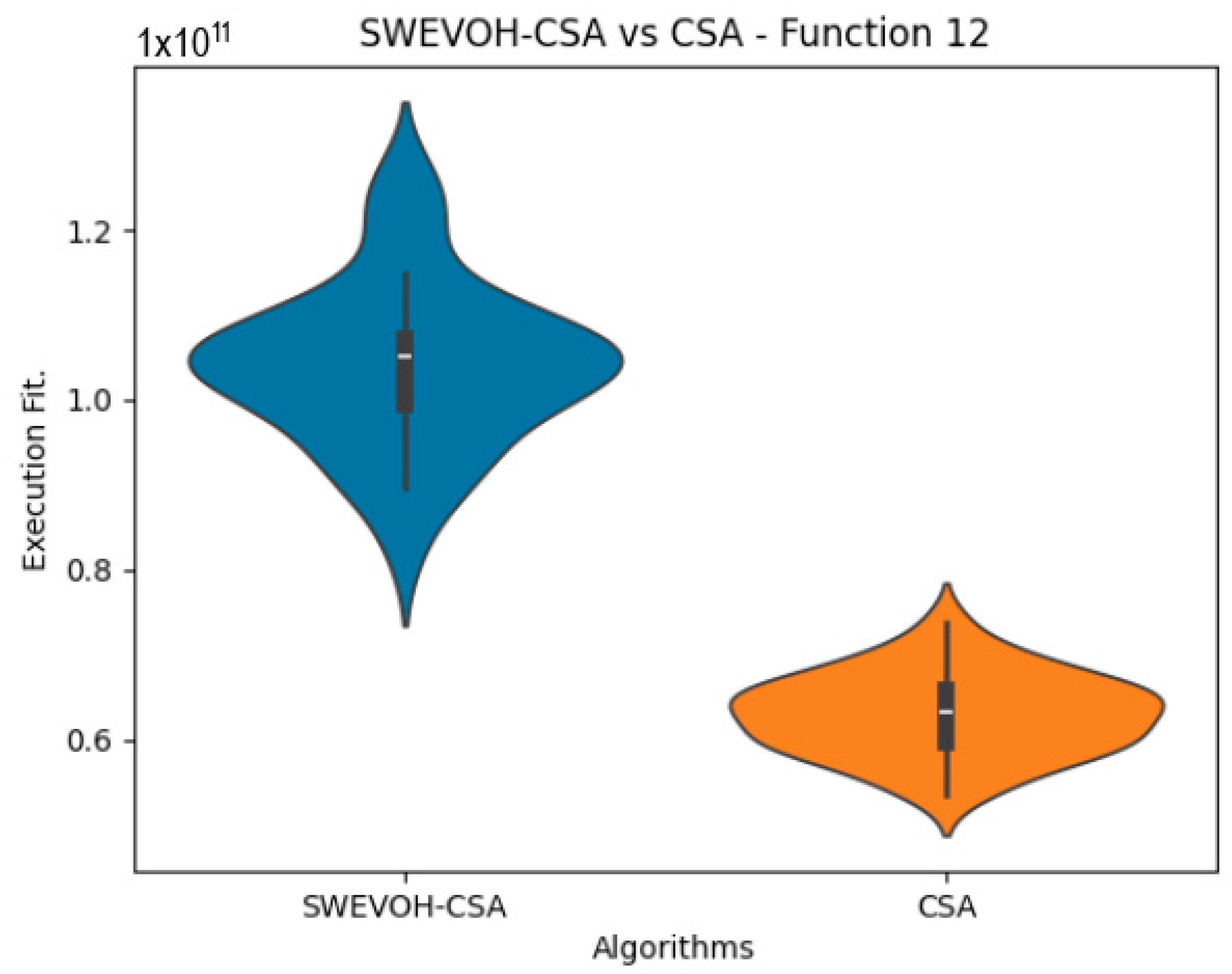
Biomimetics 09 00007 g010
Figure 11. SWEVO-CSA vs. CSA distribution on F12.
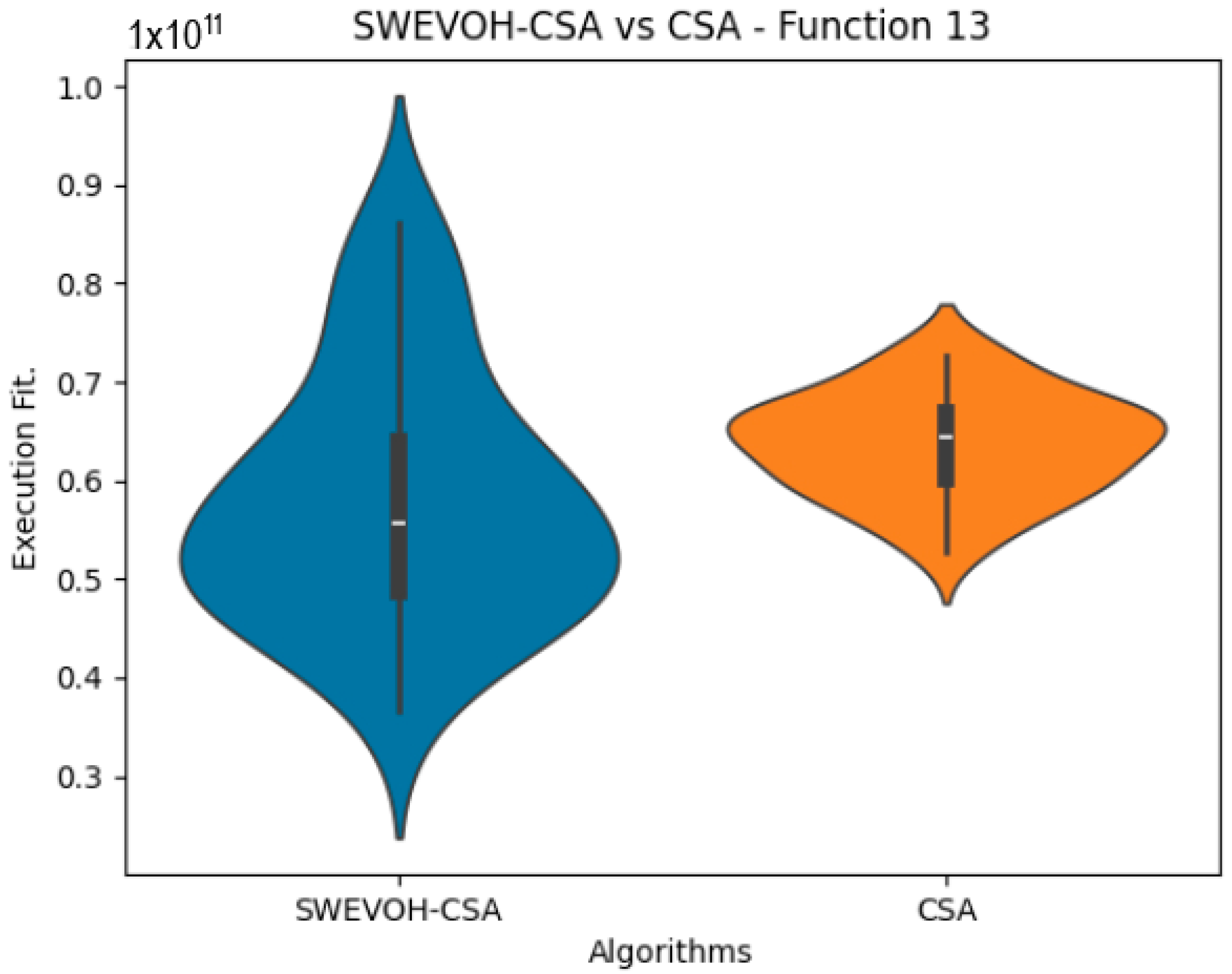
Biomimetics 09 00007 g011
Figure 12. SWEVO-CSA vs. CSA distribution on F13.
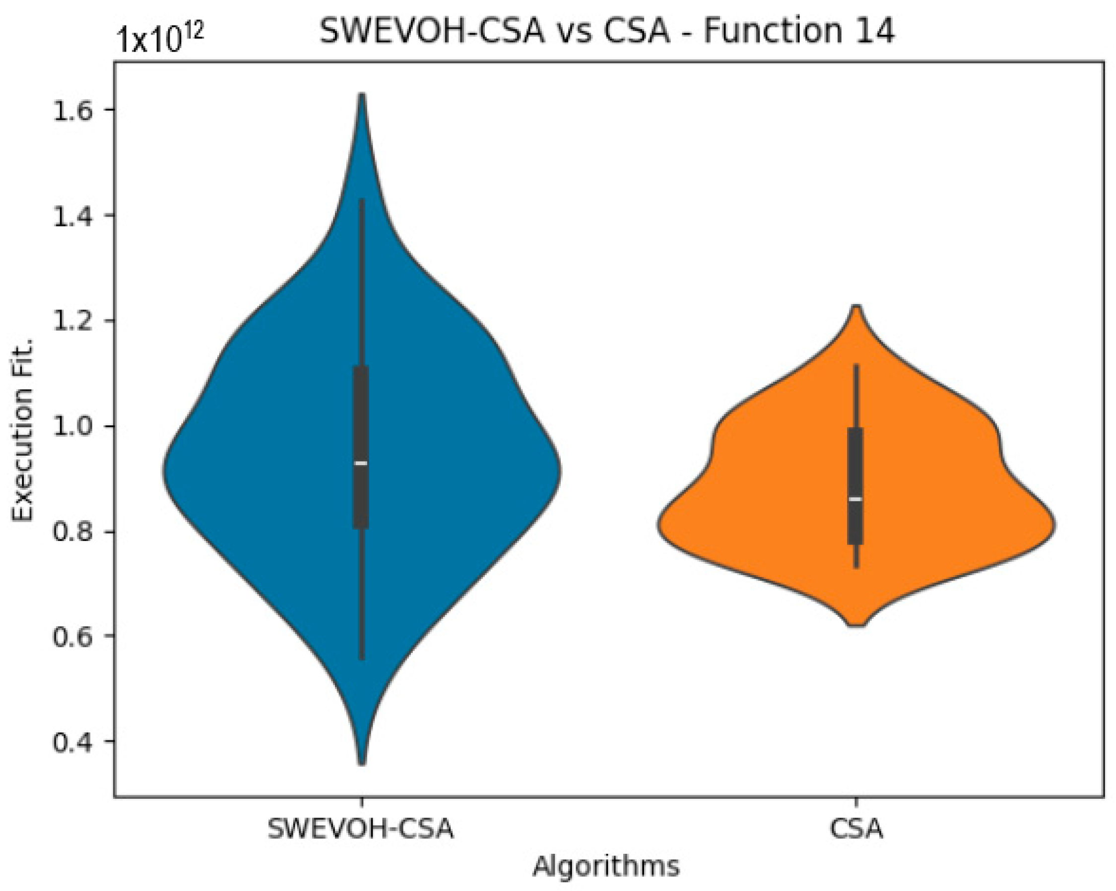
Biomimetics 09 00007 g012
Figure 13. SWEVO-CSA vs. CSA distribution on F14.
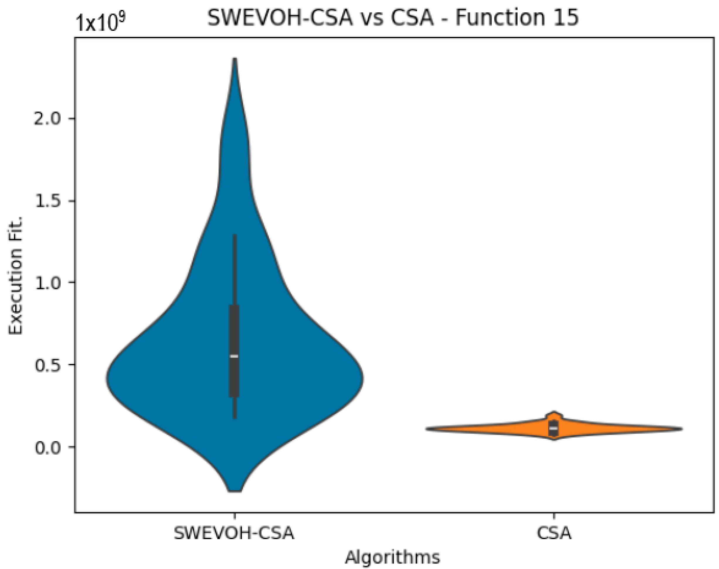
Biomimetics 09 00007 g013
Figure 14. SWEVO-CSA vs. CSA distribution on F15.
Biomimetics 09 00007 g014
Figure 15. SWEVO-BA vs. BA distribution on F10.
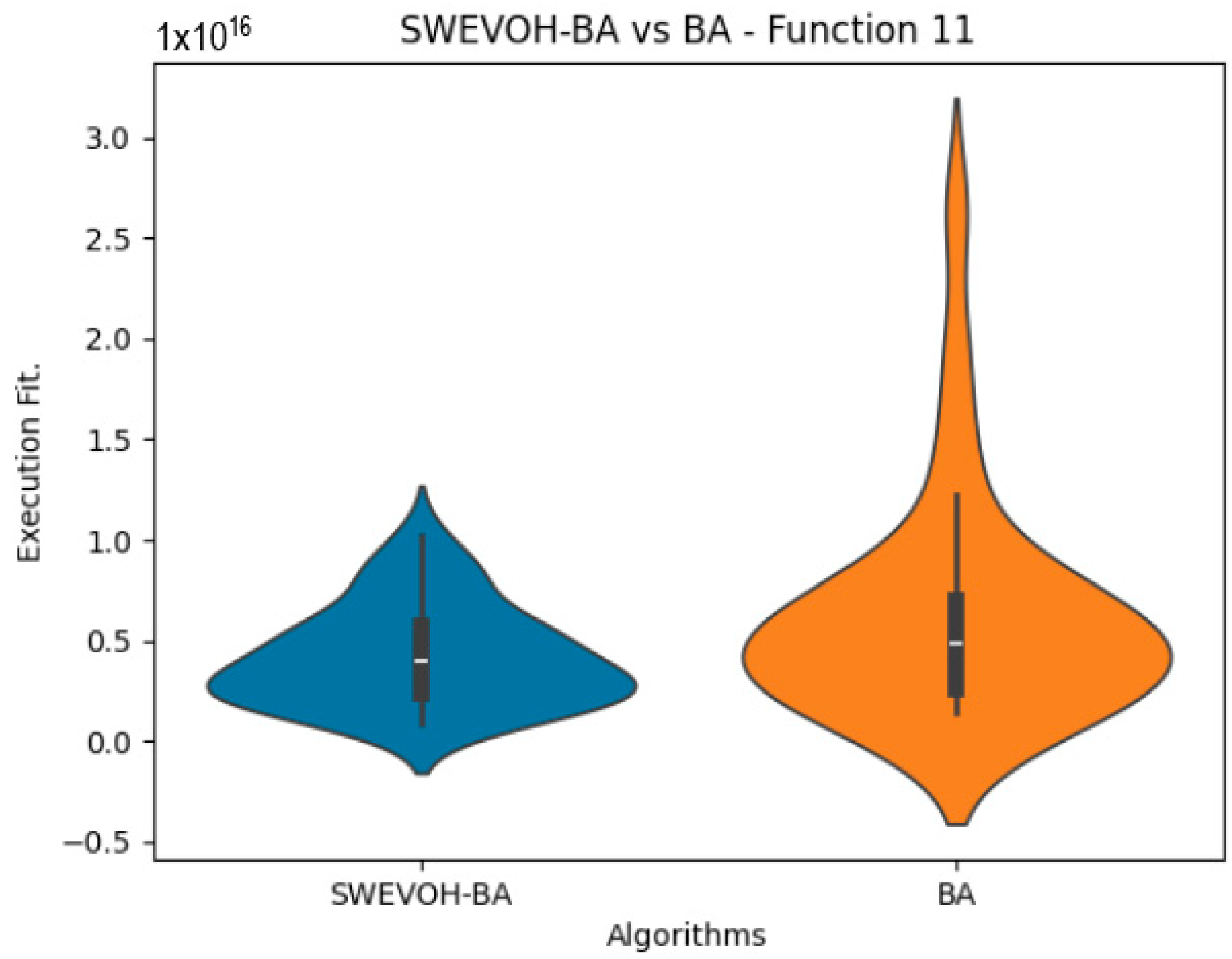
Biomimetics 09 00007 g015
Figure 16. SWEVO-BA vs. BA distribution on F11.
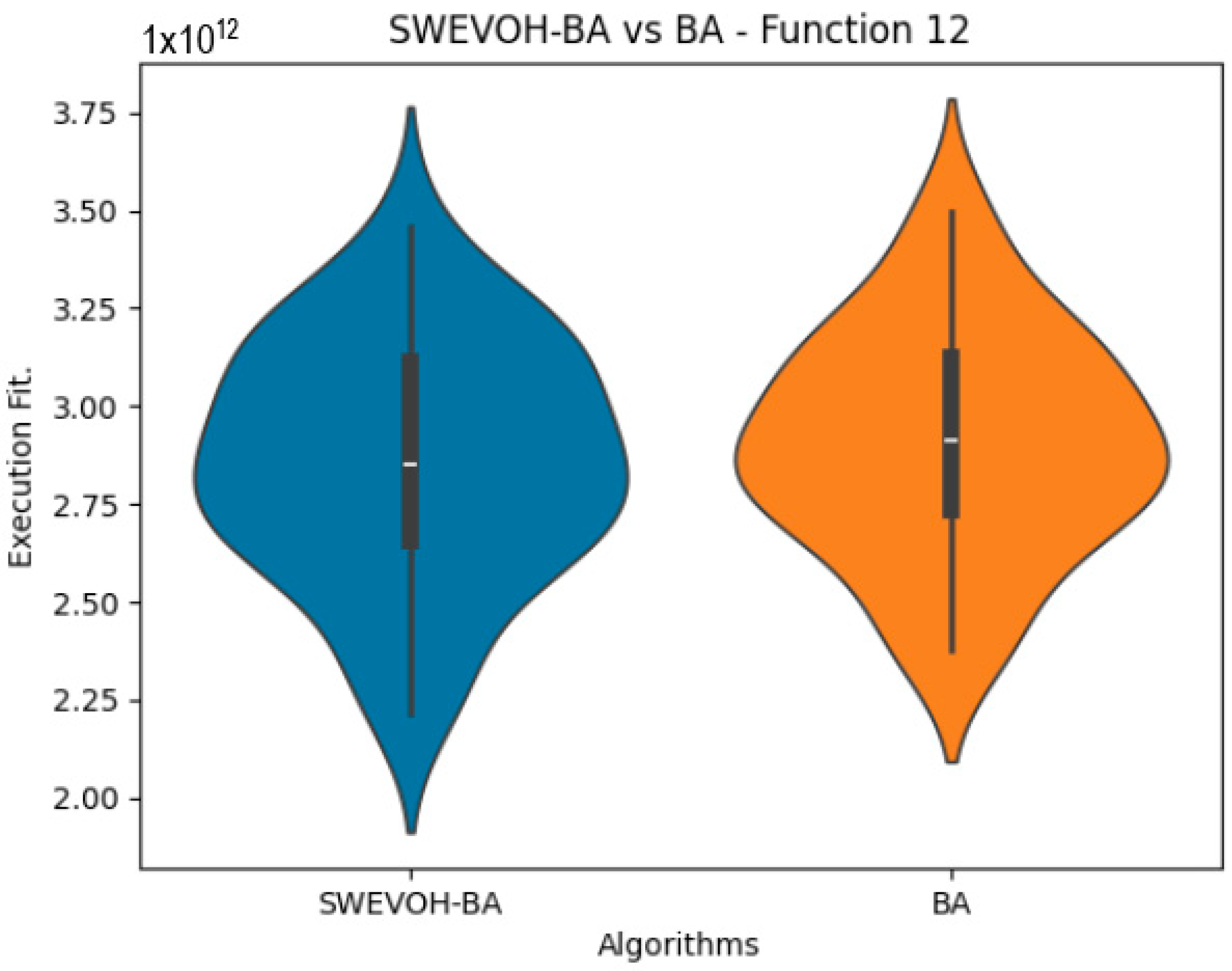
Biomimetics 09 00007 g016
Figure 17. SWEVO-BA vs. BA distribution on F12.
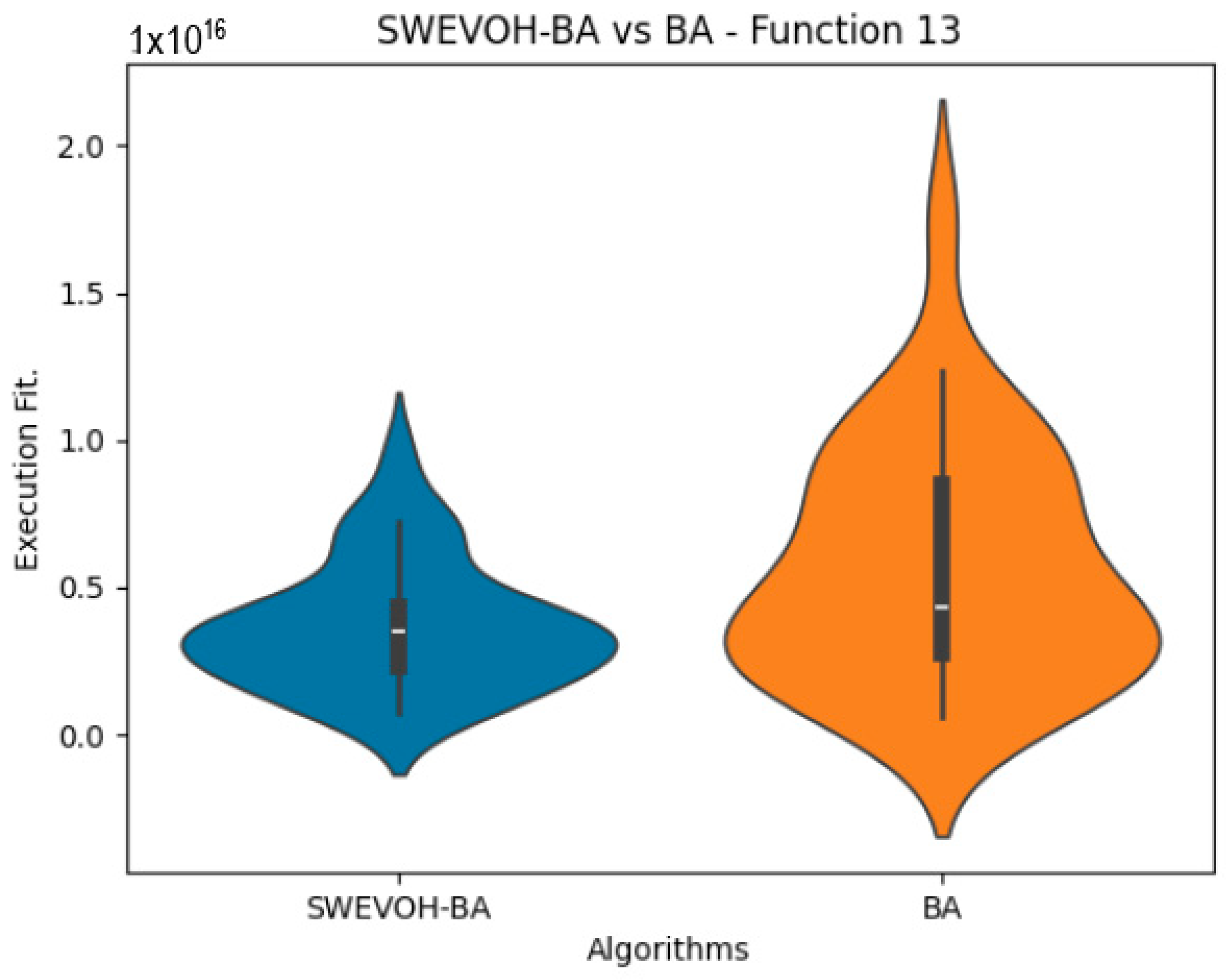
Biomimetics 09 00007 g017
Figure 18. SWEVO-BA vs. BA distribution on F13.
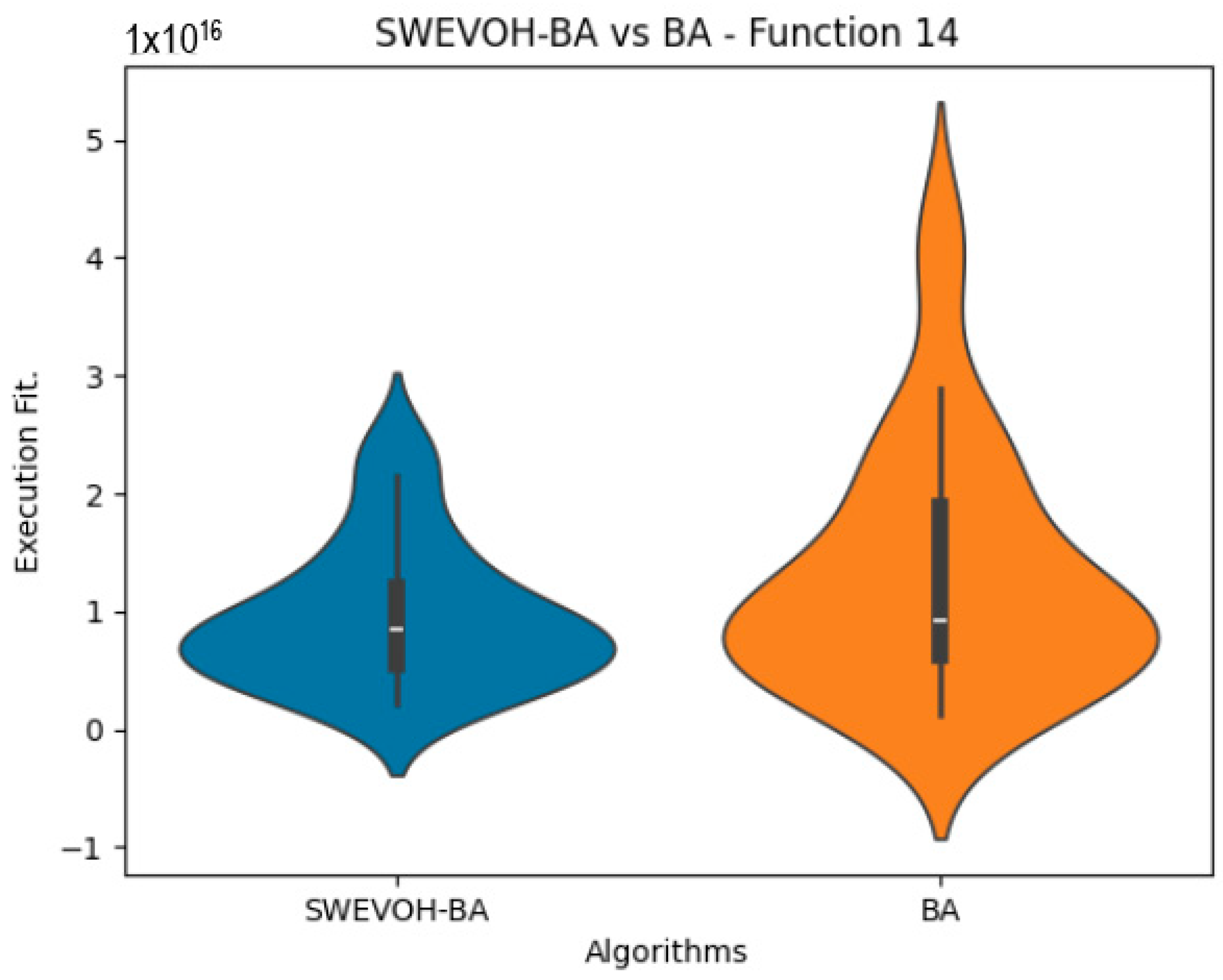
Biomimetics 09 00007 g018
Figure 19. SWEVO-BA vs. BA distribution on F14.
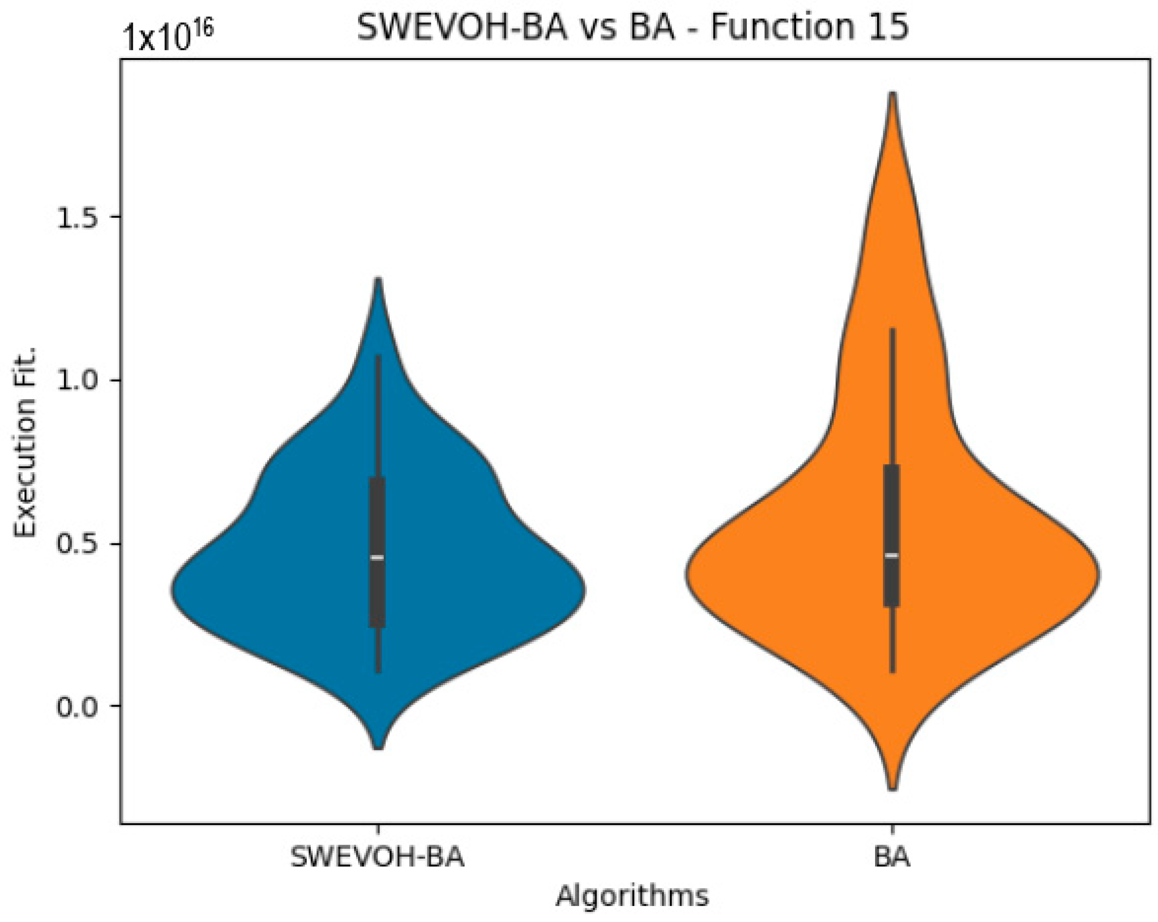
Biomimetics 09 00007 g019
Figure 20. SWEVO-BA vs. BA distribution on F15.
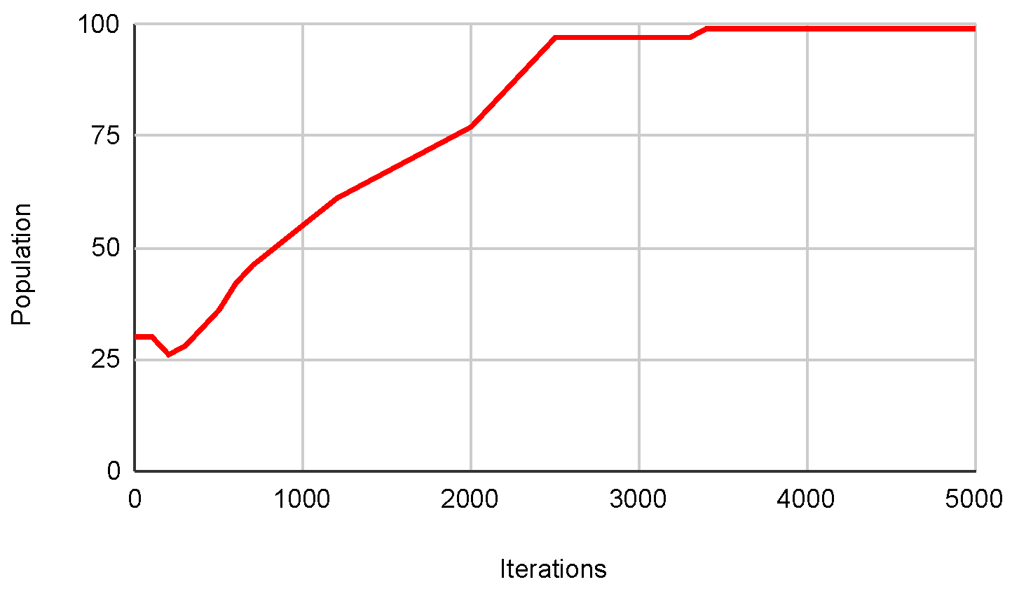
Biomimetics 09 00007 g020
Figure 21. Pop. in SWEVOH-BA—Func. 2.
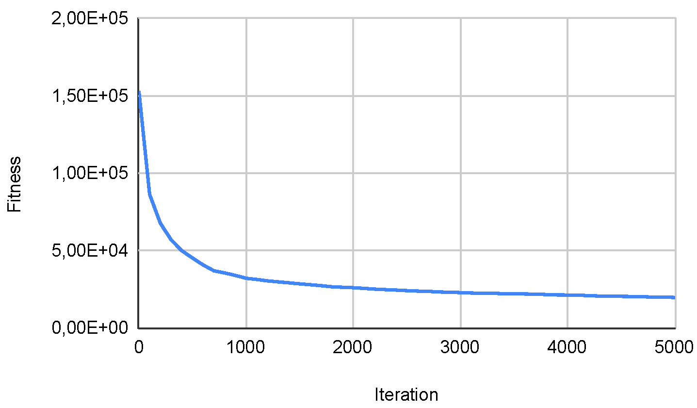
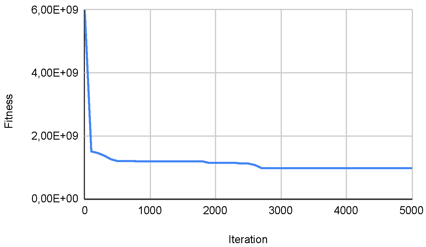
Biomimetics 09 00007 g021
Figure 22. Convg. in SWEVOH-BA—Func. 2.
Biomimetics 09 00007 g022
Figure 23. Pop. in SWEVOH-CSA—Func. 9.
Biomimetics 09 00007 g023
Figure 24. Convg. in SWEVOH-CSA—Func. 9.
Biomimetics 09 00007 g024
Table 1. SWEVOH Parameters for self-tunning population size.
Population Min–MaxImprove % AcceptedIncrement Solutions × ClusterDiff Cluster % Accepted
10–10010%25%
Table 2. SWEVOH CSA Parameters for CEC LSGO.
Population InitialAbandon Probability P a α Max Iterations L b and U b
300.250.015000Acc. to each func.
Table 3. SWEVOH BA Parameters for CEC LSGO.
Population InitialLoudness APulse Rate r α γ Max Iterations L b and U b
300.950.10.90.55000Acc. to each func.
Table 4. SWEVOH PSO Parameters for CEC LSGO.
Population InitialMax Iterations L b and U b
305000Acc. to each func.
Table 5. Comparison results between Original PSO Algorithm and Autonomous PSO Algorithm.
Original PSOAutonomous PSO
FunctionMinMaxMeanMinMaxMean
f11.69 × 10 11 5.62 × 10 11 2.33 × 10 11 6.63 × 10 9 5.52 × 10 11 7.00 × 10 10
f28.51 × 10 4 1.71 × 10 5 9.65 × 10 4 4.25 × 10 4 1.66 × 10 5 6.05 × 10 4
f32.15 × 10 1 2.18 × 10 1 2.15 × 10 1 2.13 × 10 1 2.18 × 10 1 2.14 × 10 1
f41.94 × 10 12 6.42 × 10 14 8.42 × 10 12 4.10 × 10 11 5.46 × 10 14 5.68 × 10 12
f53.03 × 10 7 2.09 × 10 8 4.37 × 10 7 2.49 × 10 7 2.44 × 10 8 4.08 × 10 7
f61.05 × 10 6 1.09 × 10 6 1.06 × 10 6 1.04 × 10 6 1.09 × 10 6 1.05 × 10 6
f73.74 × 10 12 8.76 × 10 20 1.12 × 10 18 3.12 × 10 9 1.05 × 10 21 9.51 × 10 17
f82.51 × 10 16 4.66 × 10 19 3.87 × 10 17 1.10 × 10 15 4.29 × 10 19 2.60 × 10 17
f92.34 × 10 9 3.10 × 10 10 3.57 × 10 9 2.06 × 10 9 6.48 × 10 10 3.44 × 10 9
f109.24 × 10 7 9.96 × 10 7 9.41 × 10 7 9.09 × 10 7 9.95 × 10 7 9.39 × 10 7
f116.55 × 10 14 7.04 × 10 23 8.60 × 10 20 6.83 × 10 11 3.17 × 10 23 4.19 × 10 20
f125.86 × 10 12 1.09 × 10 13 6.46 × 10 12 1.75 × 10 10 1.13 × 10 13 1.46 × 10 12
f134.30 × 10 14 1.56 × 10 23 2.80 × 10 20 2.00 × 10 11 5.48 × 10 23 3.84 × 10 20
f148.90 × 10 14 1.27 × 10 23 9.74 × 10 19 2.00 × 10 12 6.50 × 10 23 4.17 × 10 20
f151.64 × 10 16 2.08 × 10 19 3.04 × 10 17 2.61 × 10 8 2.64 × 10 19 2.07 × 10 17
Table 6. Comparison results between Original Cuckoo Search Algorithm versus Autonomous Cuckoo Search Algorithm.
Original CSAAutonomous CSA
FunctionMinMaxMeanMinMaxMean
f12.21 × 10 8 5.88 × 10 11 3.07 × 10 10 3.65 × 10 8 5.67 × 10 11 3.03 × 10 10
f22.02 × 10 4 1.67 × 10 5 3.18 × 10 4 1.97 × 10 4 1.70 × 10 5 3.16 × 10 4
f32.15 × 10 1 2.18 × 10 1 2.15 × 10 1 2.14 × 10 1 2.18 × 10 1 2.15 × 10 1
f43.48 × 10 11 8.15 × 10 14 6.91 × 10 12 2.60 × 10 11 7.74 × 10 14 6.53 × 10 12
f51.45 × 10 7 2.33 × 10 8 2.23 × 10 7 9.63 × 10 6 2.24 × 10 8 1.82 × 10 7
f61.06 × 10 6 1.09 × 10 6 1.07 × 10 6 1.05 × 10 6 1.09 × 10 6 1.06 × 10 6
f72.09 × 10 9 5.67 × 10 20 1.35 × 10 18 1.82 × 10 9 1.19 × 10 21 1.13 × 10 18
f83.04 × 10 15 5.95 × 10 19 2.96 × 10 17 1.87 × 10 15 5.07 × 10 19 2.94 × 10 17
f91.17 × 10 9 2.44 × 10 11 2.07 × 10 9 7.44 × 10 8 3.24 × 10 10 1.58 × 10 9
f109.38 × 10 7 9.95 × 10 7 9.47 × 10 7 9.29 × 10 7 9.93 × 10 7 9.44 × 10 7
f111.96 × 10 11 6.58 × 10 23 6.75 × 10 20 2.07 × 10 11 7.34 × 10 23 7.77 × 10 20
f125.35 × 10 10 1.08 × 10 13 9.27 × 10 11 7.76 × 10 10 1.10 × 10 13 9.42 × 10 11
f135.28 × 10 10 1.91 × 10 23 1.73 × 10 20 3.66 × 10 10 4.11 × 10 22 3.34 × 10 19
f147.34 × 10 11 8.14 × 10 24 5.18 × 10 21 5.59 × 10 11 1.46 × 10 23 1.63 × 10 20
f157.06 × 10 7 2.13 × 10 19 1.55 × 10 17 1.85 × 10 8 2.18 × 10 19 1.49 × 10 17
Table 7. Comparison results between Original BA versus SWEVOH -BA.
Original BATAutonomous Bat
FunctionMinMaxMeanMinMaxMean
f11.71 × 10 11 4.35 × 10 11 2.04 × 10 11 1.59 × 10 11 4.18 × 10 11 2.01 × 10 11
f22.86 × 10 4 1.31 × 10 5 3.55 × 10 4 2.55 × 10 4 1.32 × 10 5 3.45 × 10 4
f32.16 × 10 1 2.17 × 10 1 2.16 × 10 1 2.16 × 10 1 2.17 × 10 1 2.16 × 10 1
f41.49 × 10 12 8.17 × 10 13 6.16 × 10 12 2.16 × 10 12 1.03 × 10 14 5.33 × 10 12
f51.15 × 10 7 9.10 × 10 7 1.65 × 10 7 1.12 × 10 7 1.02 × 10 8 1.67 × 10 7
f61.06 × 10 6 1.08 × 10 6 1.06 × 10 6 1.06 × 10 6 1.08 × 10 6 1.06 × 10 6
f71.49 × 10 13 1.30 × 10 17 6.06 × 10 14 7.55 × 10 12 7.55 × 10 16 5.19 × 10 14
f81.96 × 10 16 3.56 × 10 18 2.33 × 10 17 1.74 × 10 16 4.98 × 10 18 2.71 × 10 17
f91.02 × 10 9 8.73 × 10 9 1.43 × 10 9 9.79 × 10 8 9.15 × 10 9 1.36 × 10 9
f109.39 × 10 7 9.75 × 10 7 9.48 × 10 7 9.36 × 10 7 9.74 × 10 7 9.47 × 10 7
f111.41 × 10 15 4.99 × 10 18 3.94 × 10 16 8.98 × 10 14 8.47 × 10 18 4.30 × 10 16
f122.38 × 10 12 8.94 × 10 12 3.03 × 10 12 2.22 × 10 12 8.93 × 10 12 3.00 × 10 12
f135.75 × 10 14 7.02 × 10 18 4.82 × 10 16 7.85 × 10 14 4.02 × 10 18 3.15 × 10 16
f141.18 × 10 15 1.07 × 10 19 7.09 × 10 16 2.18 × 10 15 1.03 × 10 19 6.92 × 10 16
f151.10 × 10 15 3.14 × 10 18 3.07 × 10 16 1.09 × 10 15 2.23 × 10 18 3.11 × 10 16
Table 8. Comparison results in similar hybrid algorithms.
Adaptive RSACSARSACSHADESWEVOH-PSOSWEVOH-CSSWEVOH-BA
Func.MeanStdMeanStdMeanStdMeanStdMeanStdMeanStd
f13.61 × 10 14 1.14 × 10 14 2.40 × 10 14 3.45 × 10 13 1.11 × 10 8 1.24 × 10 8 7.00 × 10 10 8.30 × 10 10 3.03 × 10 10 7.81 × 10 10 2.01 × 10 11 3.04 × 10 10
f27.96 × 10 7 3.94 × 10 7 5.47 × 10 7 1.19 × 10 7 1.41 × 10 7 9.22 × 10 5 6.05 × 10 4 1.67 × 10 4 3.16 × 10 4 1.97 × 10 4 3.45 × 10 4 1.31 × 10 4
f32.14 × 10 4 1.89 × 10 2 2.12 × 10 4 1.05 × 10 2 1.68 × 10 4 6.52 × 10 2 2.14 × 10 1 9.04 × 10 2 2.15 × 10 1 5.61 × 10 2 2.16 × 10 1 1.39 × 10 2
f41.24 × 10 17 9.29 × 10 16 5.21 × 10 16 3.28 × 10 16 1.18 × 10 14 1.26 × 10 14 5.68 × 10 12 3.64 × 10 13 6.53 × 10 12 4.63 × 10 13 5.33 × 10 12 6.67 × 10 12
f58.63 × 10 10 3.48 × 10 10 5.80 × 10 10 9.49 × 10 9 2.05 × 10 9 3.44 × 10 8 4.08 × 10 7 1.59 × 10 7 1.82 × 10 7 1.70 × 10 7 1.67 × 10 7 9.28 × 10 6
f61.06 × 10 9 1.29 × 10 7 1.04 × 10 9 9.18 × 10 6 7.22 × 10 7 3.01 × 10 7 1.05 × 10 6 8.04 × 10 3 1.06 × 10 6 3.52 × 10 3 1.06 × 10 6 2.21 × 10 3
f71.87 × 10 21 8.95 × 10 21 4.11 × 10 18 6.76 × 10 18 5.06 × 10 10 1.98 × 10 11 9.51 × 10 17 2.69 × 10 19 1.13 × 10 18 3.05 × 10 19 5.19 × 10 14 4.28 × 10 15
f84.42 × 10 21 4.72 × 10 21 3.00 × 10 21 2.47 × 10 21 5.80 × 10 18 4.12 × 10 18 2.60 × 10 17 2.05 × 10 18 2.94 × 10 17 2.66 × 10 18 2.71 × 10 17 3.87 × 10 17
f91.03 × 10 13 9.45 × 10 12 5.32 × 10 12 1.56 × 10 12 2.09 × 10 11 2.19 × 10 10 3.44 × 10 9 2.48 × 10 9 1.58 × 10 9 2.14 × 10 9 1.36 × 10 9 7.68 × 10 8
f109.48 × 10 10 7.66 × 10 8 9.44 × 10 10 6.81 × 10 8 1.02 × 10 9 4.34 × 10 8 9.39 × 10 7 1.12 × 10 6 9.44 × 10 7 7.76 × 10 5 9.47 × 10 7 5.10 × 10 5
f117.29 × 10 22 1.97 × 10 23 1.70 × 10 20 4.62 × 10 20 3.42 × 10 10 1.73 × 10 10 4.19 × 10 20 1.03 × 10 22 7.77 × 10 20 2.07 × 10 22 4.30 × 10 16 4.22 × 10 17
f126.34 × 10 15 3.36 × 10 15 2.57 × 10 15 6.39 × 10 14 8.07 × 10 8 2.33 × 10 9 1.46 × 10 12 2.03 × 10 12 9.42 × 10 11 1.58 × 10 12 3.00 × 10 12 8.30 × 10 11
f133.58 × 10 23 1.73 × 10 24 3.58 × 10 20 6.87 × 10 20 1.56 × 10 11 6.80 × 10 11 3.84 × 10 20 1.38 × 10 22 3.34 × 10 19 1.04 × 10 21 3.15 × 10 16 2.26 × 10 17
f141.89 × 10 22 4.07 × 10 22 7.97 × 10 20 1.82 × 10 21 1.56 × 10 12 8.43 × 10 12 4.17 × 10 20 1.64 × 10 22 1.63 × 10 20 3.93 × 10 21 6.92 × 10 16 5.20 × 10 17
f152.50 × 10 21 4.90 × 10 21 9.04 × 10 18 1.17 × 10 19 1.25 × 10 10 5.48 × 10 9 2.07 × 10 17 1.68 × 10 18 1.49 × 10 17 1.29 × 10 18 3.11 × 10 16 1.97 × 10 17
Table 9. PSO p-values for function 1.
SWEVOH-PSOPSO
SWEVOH-PSO×SWS
PSO7.01 × 10 3 ×
Table 10. PSO p-values for function 2.
SWEVOH-PSOPSO
SWEVOH-PSO×SWS
PSOSWS×
Table 11. PSO p-values for function 3.
SWEVOH-PSOPSO
SWEVOH-PSO×7.01 × 10 3
PSOSWS×
Table 12. PSO p-values for function 4.
SWEVOH-PSOPSO
SWEVOH-PSO×1.86 × 10 16
PSOSWS×
Table 13. PSO p-values for function 5.
SWEVOH-PSOPSO
SWEVOH-PSO×6.21 × 10 4
PSOSWS×
Table 14. PSO p-values for function 6.
SWEVOH-PSOPSO
SWEVOH-PSO×1.67 × 10 16
PSOSWS×
Table 15. PSO p-values for function 7.
SWEVOH-PSOPSO
SWEVOH-PSO×SWS
PSOSWS×
Table 16. PSO p-values for function 8.
SWEVOH-PSOPSO
SWEVOH-PSO×SWS
PSO1.51 × 10 15 ×
Table 17. PSO p-values for function 9.
SWEVOH-PSOPSO
SWEVOH-PSO×5.93 × 10 5
PSOSWS×
Table 18. PSO p-values for function 10.
SWEVOH-PSOPSO
SWEVOH-PSO×3.78 × 10 10
PSOSWS×
Table 19. PSO p-values for function 11.
SWEVOH-PSOPSO
SWEVOH-PSO×SWS
PSOSWS×
Table 20. PSO p-values for function 12.
SWEVOH-PSOPSO
SWEVOH-PSO×SWS
PSO6.97 × 10 3 ×
Table 21. PSO p-values for function 13.
SWEVOH-PSOPSO
SWEVOH-PSO×2.90 × 10 16
PSOSWS×
Table 22. PSO p-values for function 14.
SWEVOH-PSOPSO
SWEVOH-PSO×SWS
PSOSWS×
Table 23. PSO p-values for function 15.
SWEVOH-PSOPSO
SWEVOH-PSO×SWS
PSO8.49 × 10 3 ×
Table 24. CSA p-values for function 1.
SWEVOH-CSACSA
SWEVOH-CSA×SWS
CSA7.01 × 10 12 ×
Table 25. CSA p-values for function 2.
SWEVOH-CSACSA
SWEVOH-CSA×SWS
CSASWS×
Table 26. CSA p-values for function 3.
SWEVOH-CSACSA
SWEVOH-CSA×7.01 × 10 12
CSASWS×
Table 27. CSA p-values for function 4.
SWEVOH-CSACSA
SWEVOH-CSA×1.86 × 10 3
CSASWS×
Table 28. CSA p-values for function 5.
SWEVOH-CSACSA
SWEVOH-CSA×6.21 × 10 11
CSASWS×
Table 29. CSA p-values for function 6.
SWEVOH-CSACSA
SWEVOH-CSA×1.67 × 10 2
CSASWS×
Table 30. CSA p-values for function 7.
SWEVOH-CSACSA
SWEVOH-CSA×SWS
CSASWS×
Table 31. CSA p-values for function 8.
SWEVOH-CSACSA
SWEVOH-CSA×SWS
CSA1.51 × 10 2 ×
Table 32. CSA p-values for function 9.
SWEVOH-CSACSA
SWEVOH-CSA×5.93 × 10 10
CSASWS×
Table 33. CSA p-values for function 10.
SWEVOH-CSACSA
SWEVOH-CSA×3.78 × 10 6
CSASWS×
Table 34. CSA p-values for function 11.
SWEVOH-CSACSA
SWEVOH-CSA×SWS
CSASWS×
Table 35. CSA p-values for function 12.
SWEVOH-CSACSA
SWEVOH-CSA×SWS
CSA6.97 × 10 12 ×
Table 36. CSA p-values for function 13.
SWEVOH-CSACSA
SWEVOH-CSA×2.90 × 10 3
CSASWS×
Table 37. CSA p-values for function 14.
SWEVOH-CSACSA
SWEVOH-CSA×SWS
CSASWS×
Table 38. CSA p-values for function 15.
SWEVOH-CSACSA
SWEVOH-CSA×SWS
CSA8.49 × 10 12 ×
Table 39. BA p-values for function 1.
SWEVOH-BABA
SWEVOH-BA×SWS
BASWS×
Table 40. BA p-values for function 2.
SWEVOH-BABA
SWEVOH-BA×1.48 × 10 16
BASWS×
Table 41. BA p-values for function 3.
SWEVOH-BABA
SWEVOH-BA×7.43 × 10 15
BASWS×
Table 42. BA p-values for function 4.
SWEVOH-BABA
SWEVOH-BA×3.58 × 10 15
BASWS×
Table 43. BA p-values for function 5.
SWEVOH-BABA
SWEVOH-BA×SWS
BASWS×
Table 44. BA p-values for function 6.
SWEVOH-BABA
SWEVOH-BA×4.21 × 10 14
BASWS×
Table 45. BA p-values for function 7.
SWEVOH-BABA
SWEVOH-BA×2.96 × 10 16
BASWS×
Table 46. BA p-values for function 8.
SWEVOH-BABA
SWEVOH-BA×SWS
BASWS×
Table 47. BA p-values for function 9.
SWEVOH-BABA
SWEVOH-BA×4.56 × 10 15
BASWS×
Table 48. BA p-values for function 10.
SWEVOH-BABA
SWEVOH-BA×2.67 × 10 16
BASWS×
Table 49. BA p-values for function 11.
SWEVOH-BABA
SWEVOH-BA×SWS
BASWS×
Table 50. BA p-values for function 12.
SWEVOH-BABA
SWEVOH-BA×SWS
BASWS×
Table 51. BA p-values for function 13.
SWEVOH-BABA
SWEVOH-BA×2.36 × 10 16
BASWS×
Table 52. BA p-values for function 14.
SWEVOH-BABA
SWEVOH-BA×SWS
BASWS×
Table 53. BA p-values for function 15.
SWEVOH-BABA
SWEVOH-BA×SWS
BASWS×
Disclaimer/Publisher’s Note: The statements, opinions and data contained in all publications are solely those of the individual author(s) and contributor(s) and not of MDPI and/or the editor(s). MDPI and/or the editor(s) disclaim responsibility for any injury to people or property resulting from any ideas, methods, instructions or products referred to in the content.

