

Differential Mutation Incorporated Quantum Honey Badger Algorithm with Dynamic Opposite Learning and Laplace Crossover for Fuzzy Front-End Product Design
Abstract
1. Introduction

| Algorithms | Abbrev. | Inspiration |
|---|---|---|
| Particle Swarm Optimization | PSO [23] | The predation behavior of birds |
| Genetic algorithms | GA [5] | Darwin’s theory |
| Gravitational Search Algorithm | GSA [6] | The interaction law |
| Teaching Learning-Based Optimization | TLBO [8] | The effect of influence of a teacher on learners |
| Ant Colony Optimization | ACO [24] | The foraging behavior of ants |
| Bat Algorithm | BA [25] | The echolocation behavior of bats |
| Cuckoo Search algorithm | CS [26] | The reproductive characteristics of cuckoo birds |
| Gray Wolf Optimization | GWO [27] | The leadership hierarchy and hunting mechanism |
| Whale Optimization Algorithm | WOA [28] | The bubble-net hunting behavior of humpback whales |
| Salp Swarm Algorithm | SSA [29] | The swarming behaviour of salps when navigating and foraging in oceans |
| Sea-horse Optimizer | SHO [30] | The movement, predation, and breeding behaviors of sea horses |
| Reptile Search Algorithm | RSA [31] | The hunting behavior of crocodiles |
| Tunicate Swarm Algorithm | TSA [33] | The group behavior of tunicates in the ocean |
| Sine Cosine Algorithm | SCA [32] | Based on mathematical models of sine and cosine functions |
| Wild Horse Optimizer | WHO [34] | The decency behaviour of the horse |
| Arithmetic Optimization Algorithm | AOA [35] | The main arithmetic operators in mathematics |
| Moth Flame Optimization | MFO [36] | The navigation method of moths |
| Honey Badger Algorithm | HBA [37] | The intelligent foraging behavior of honey badger |
- (a)
- A dynamic opposite learning strategy was adopted for HBA initialization to enhance the diversity of the population and quality of candidate solution for performance improvement of the original HBA, and increases the convergence speed of the algorithm.
- (b)
- Combining differential mutation operations to increase the diversity of individual populations, enhance the HBA’s capability to jump out of local optima, and to some extent increase the precision of HBA.
- (c)
- Local quantum search and dynamic Laplacian crossover operators are selectively used in the mining and honey mining stages to balance the development and exploration stages of the algorithm.
- (d)
- Performance testing and analysis of EHBA were conducted on test sets CEC2017, CEC2020, and CEC2022, respectively. The feasibility, stability, and high accuracy of the proposed method have been verified through existing test sets. Improved new algorithms EHBA were adopted to design and solve three typical engineering practical cases, further verifying the practicality of EHBA.
2. Theoretical Basis of Honey Badger Algorithm
2.1. Population Initialization Stage
2.2. Digging Stage (Exploration)
2.2.1. Definition of the Intensity I
2.2.2. Update Density Factor α
2.2.3. Definition of the Search Orientation F
2.2.4. Update Location of Digging Stage
2.3. Honey Harvesting Stage (Exploitation)
3. An Enhanced Honey Badger Algorithm Combining Multiple Strategies
3.1. Dynamic Opposite Learning Strategy
3.2. Differential Mutation Operation
- Mutations. Mutation refers to calculating the weighted position difference between two individuals in a population, then adding the position of a random individual to generate a mutated individual. The specific mutation procedures can be described with Equation (11).
- Crossover. By using some parts of the present population and corresponding parts of the mutant population, and exchanging them in accordance with certain rules, it is possible to make a cross population that can enrich the variety of the species in the population.
- Selection. If the fitness value of the cross vector is not inferior to the fitness value of the target individuals , then replace the target individual with the cross vector in the next generation.
3.3. Quantum Local Search
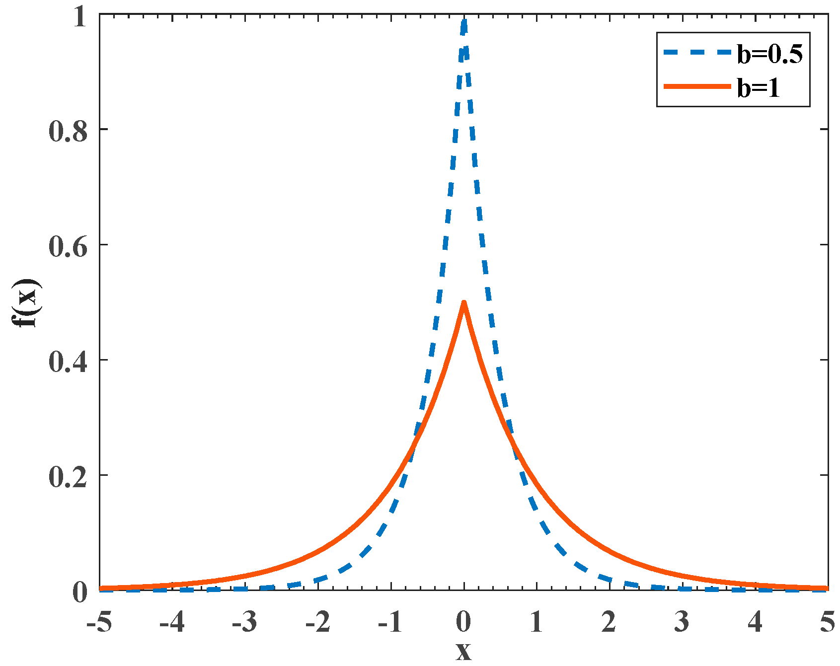
3.4. Dynamic Laplace Crossover
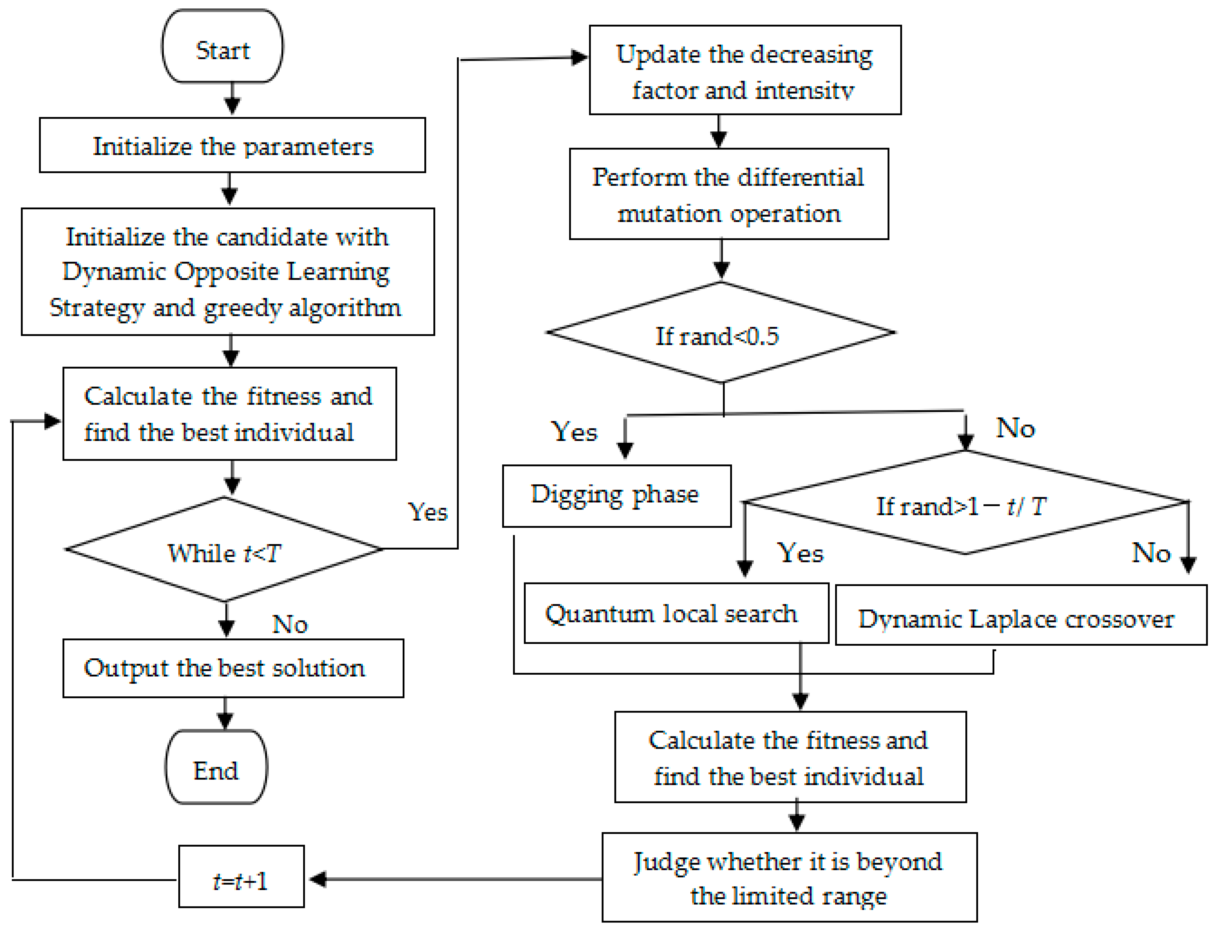
3.5. The Specific Steps of the Enhanced Honey Badger Algorithm
| Algorithm 1: The Proposed EHBA |
| Input: The parameters of HBA such as β, C, N, Dim, and maximum iterations T. |
| Output: Optimal fitness value. |
| Random Initialization |
| Construct the new population through dynamic opposite learning strategy. For i = 1 to N do r8 = rand(0,1), r9 = rand(0,1), For j = 1 to Dim do Check the boundaries. |
| Using greedy algorithm to select the best initial population from 2N populations |
| Evaluate all fitness value F(Pi), i = 1, 2, …, N. Save best position PBest and FBest. |
| While (t < T) do |
| Renew the decreasing factor α by Equation (6). |
| For i =1 to N do |
| Calculate the intensity Ii by Equation (4). |
| Perform differential mutation operation with Equations (11)–(13): For i = 1 to N do Perform mutation by Equation (11); End For i = 1 to N For j = 1 to Dim do Perform crossover by Equation (12); End End For i = 1 to N For j = 1 to Dim do Perform selection by Equation (13); End End |
| If r < 0.5 then |
| Replace the location Pnew by Equation (8). |
| Else |
| Quantum Local Search: Perform Equations (14)–(16) |
| Else |
| Dynamic Laplace Crossover: |
| if r1 < 1 − t/T then Renewed the honey badger location with Equation (21). Else Renewed the honey badger location with Equation (22). End if |
| End if |
| Evaluate new position |
| If Fnew ≤ F(Pi) then |
| Let Pi = Pnew and Fi = Fnew. |
| End if |
| If Fnew ≤ FBest then |
| Make PBest = Pnew and FBest = Fnew. |
| End if |
| End For |
| Verify the honey badger’s boundaries. |
| Refresh Honey Badger’s location and most best location (P*) |
| t = t + 1 |
| End while |
3.6. The Complexity Analysis
4. Numerical Experiment and Analysis Results
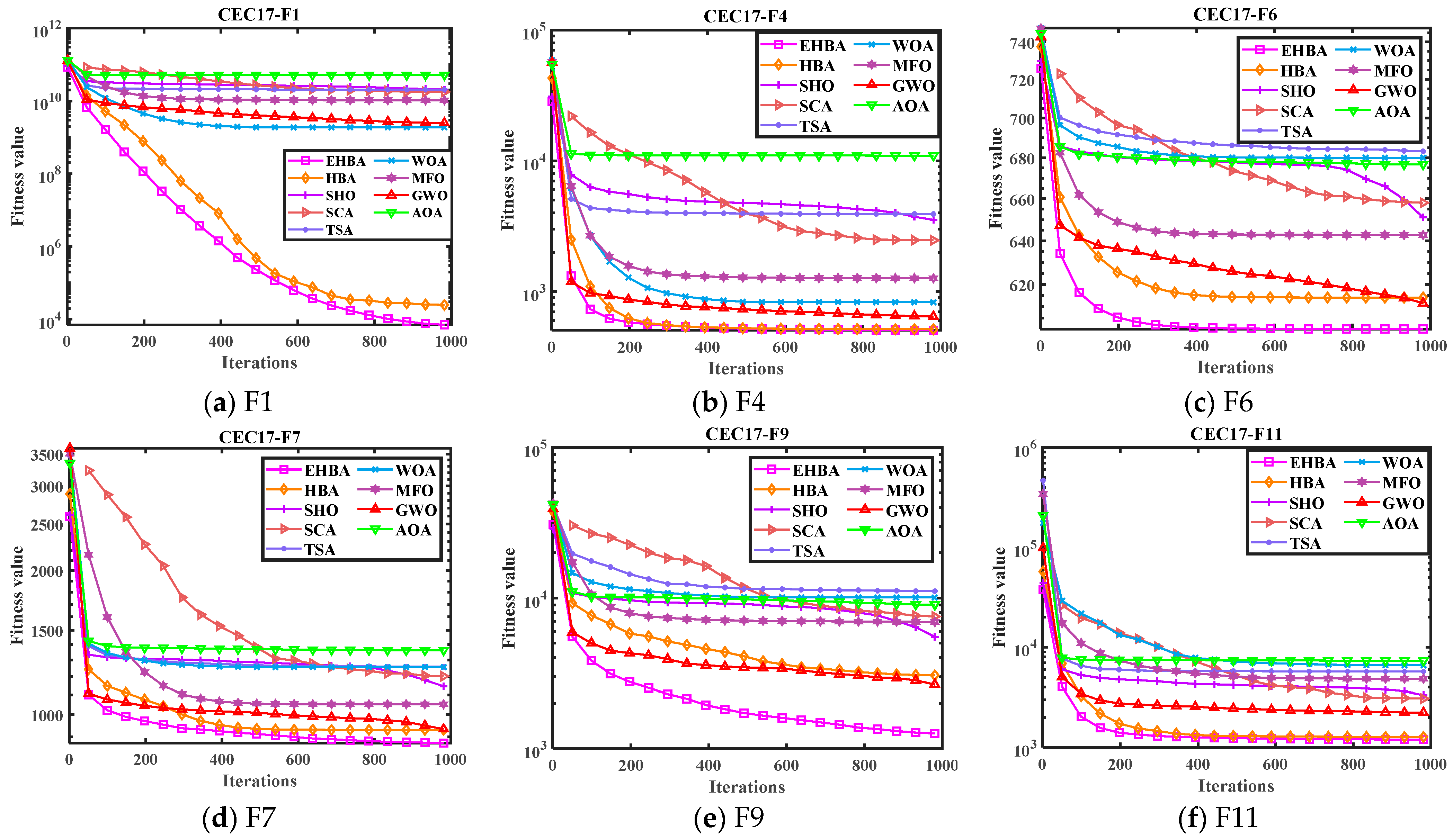
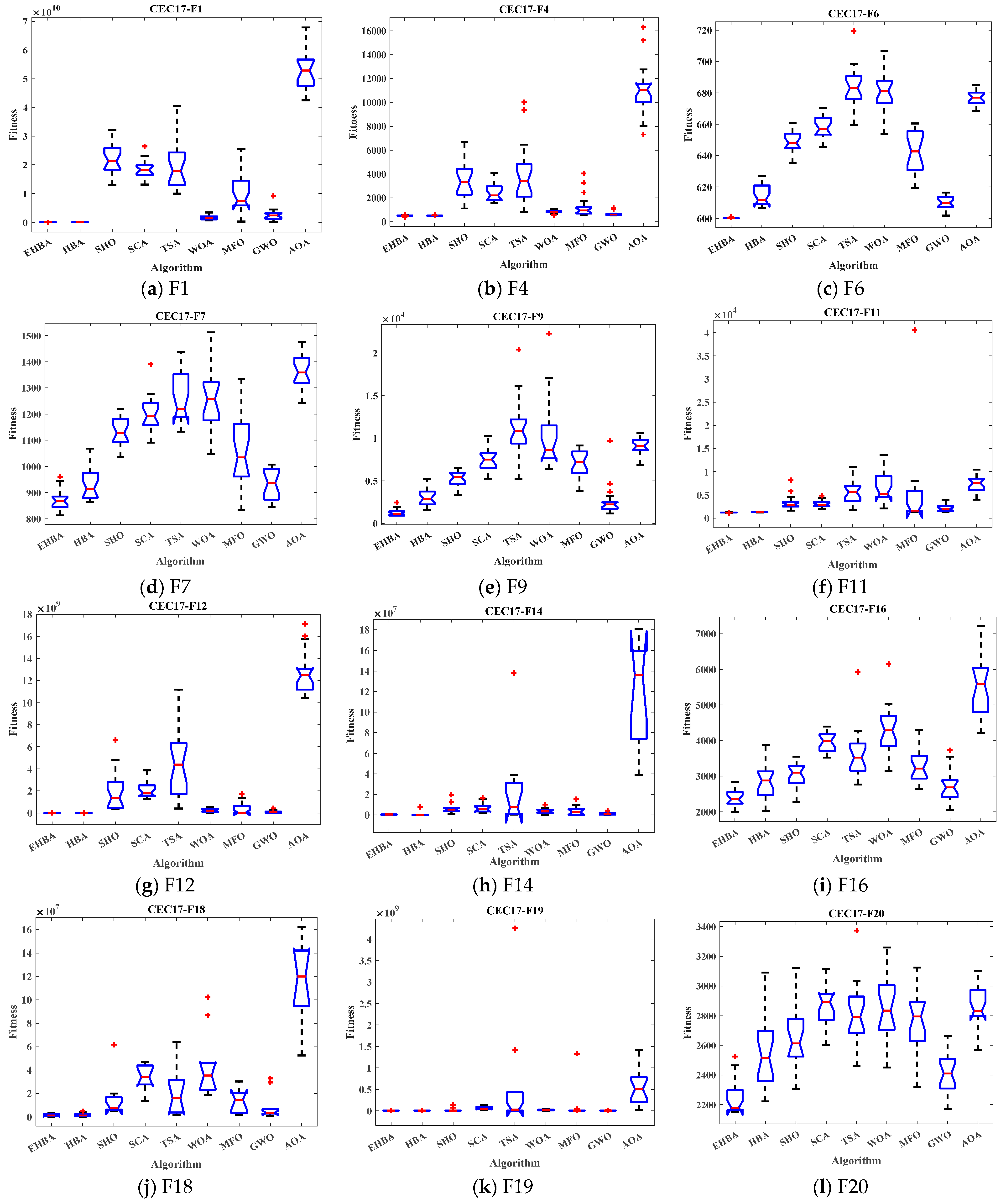
4.1. Experiment and Analysis on the CEC2017 Test Set
4.2. Experiment and Analysis on the CEC2020 Test Set
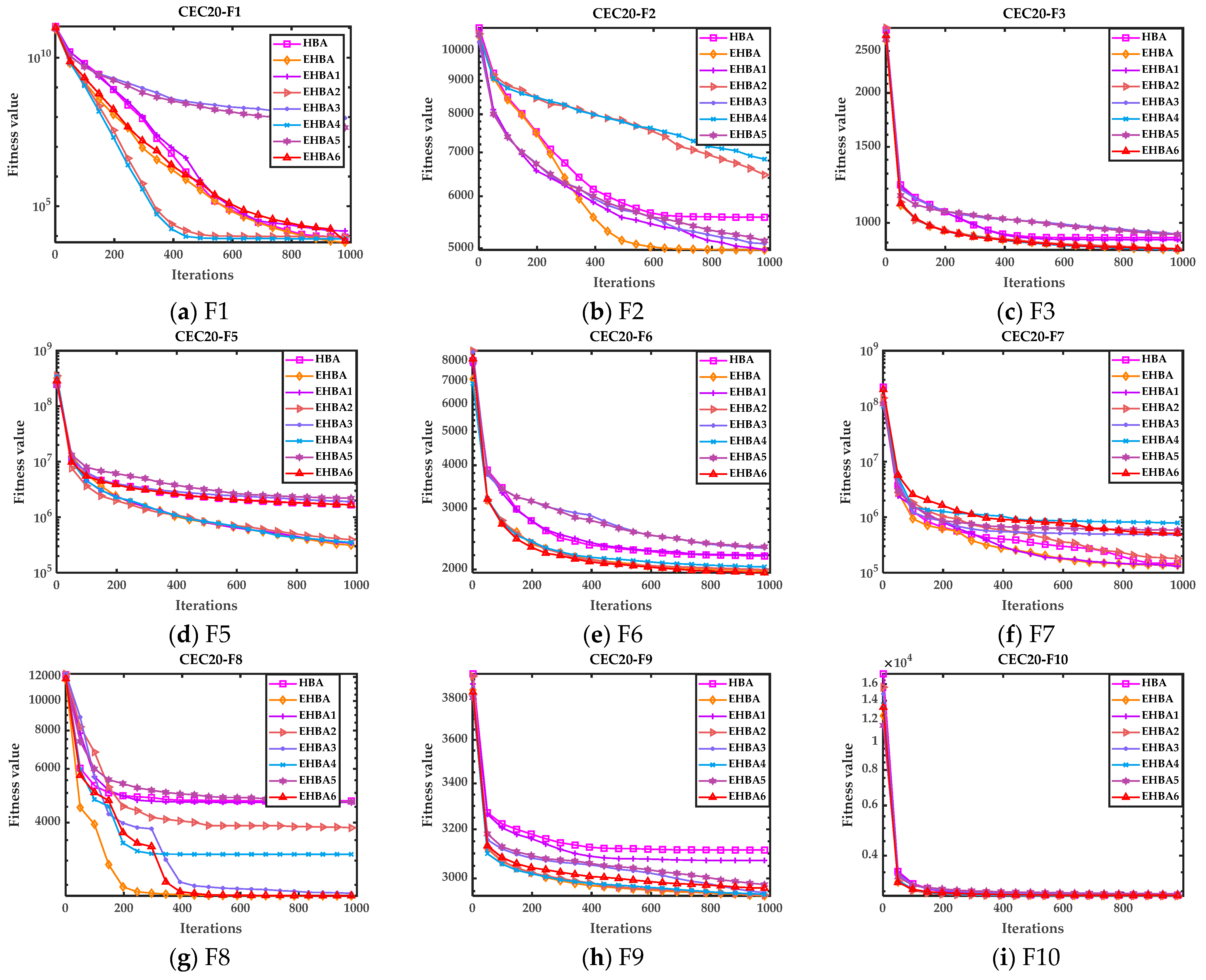
4.2.1. The Ablation Experiments of EHBA
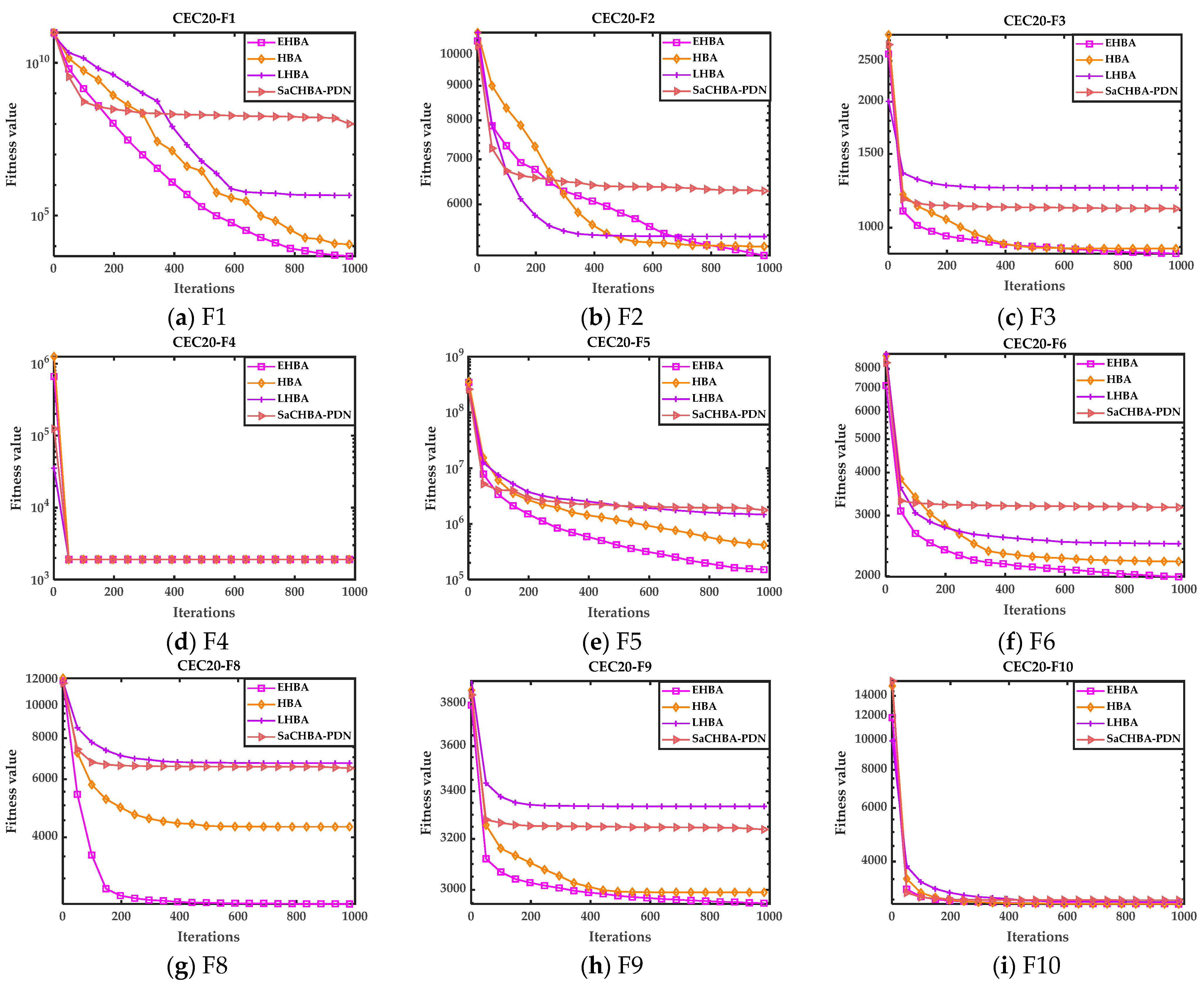
4.2.2. Comparison Experiment between Other HBA Variant Algorithms and EHBA
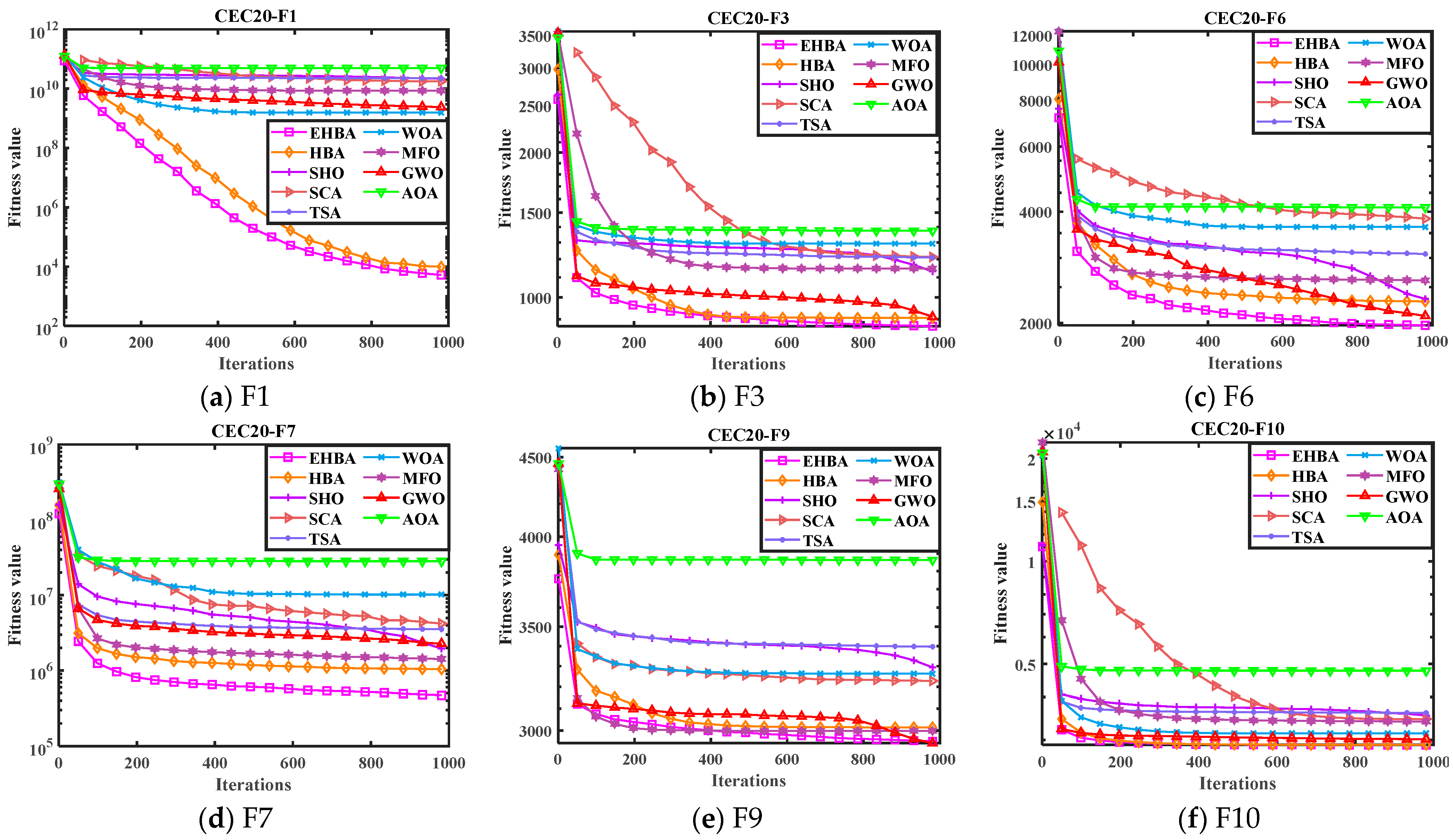
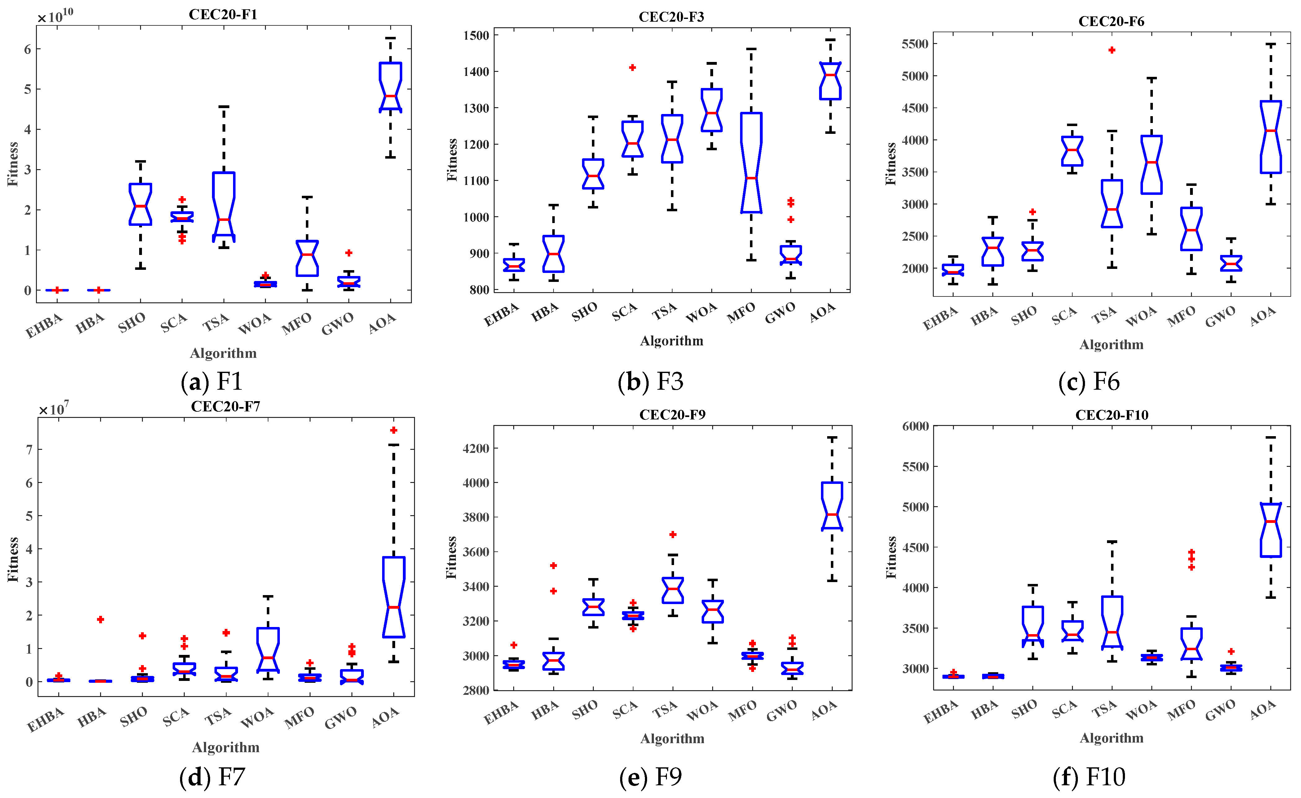
4.2.3. Comparison Experiments of EHBA and Other Intelligent Algorithms
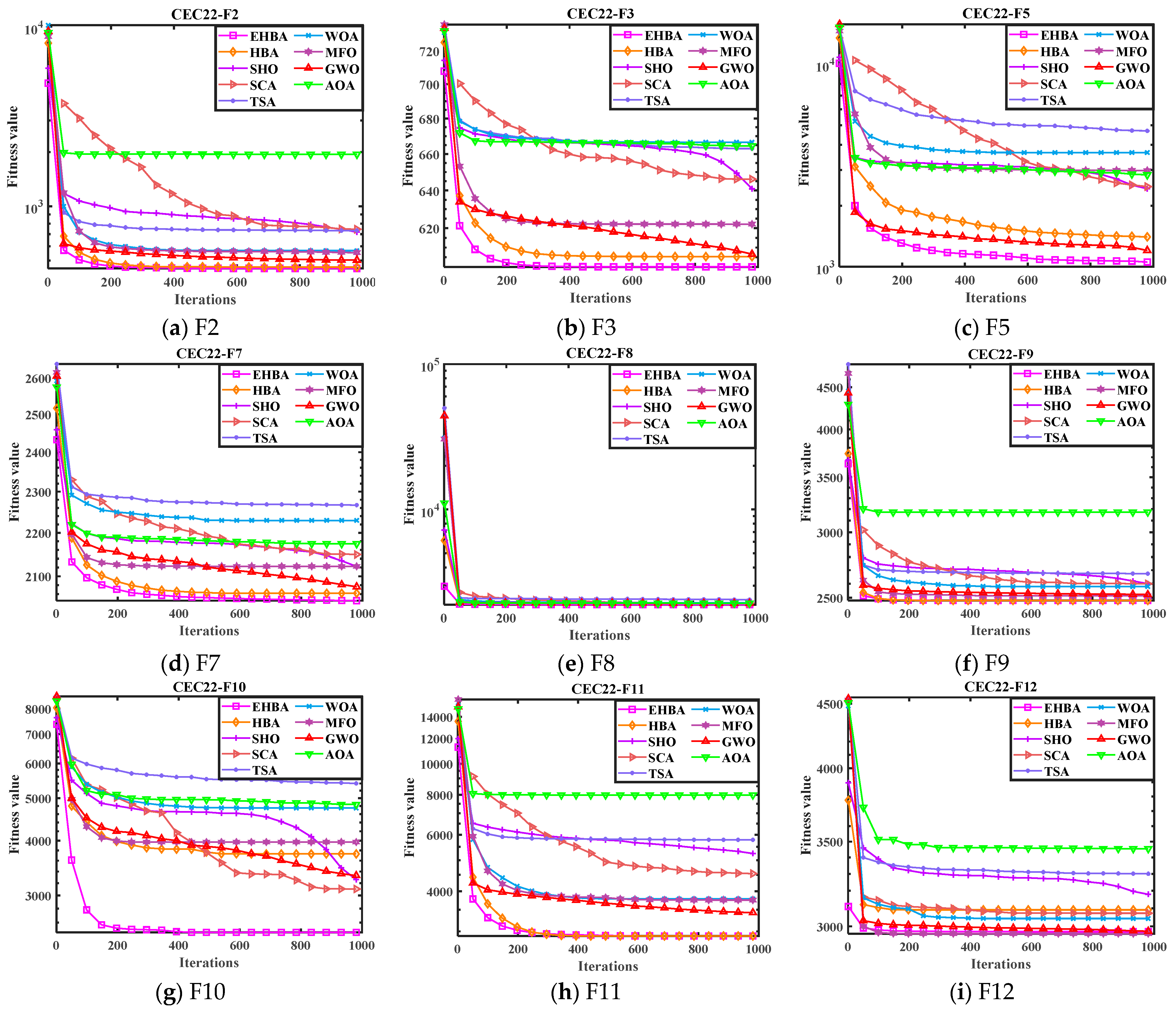
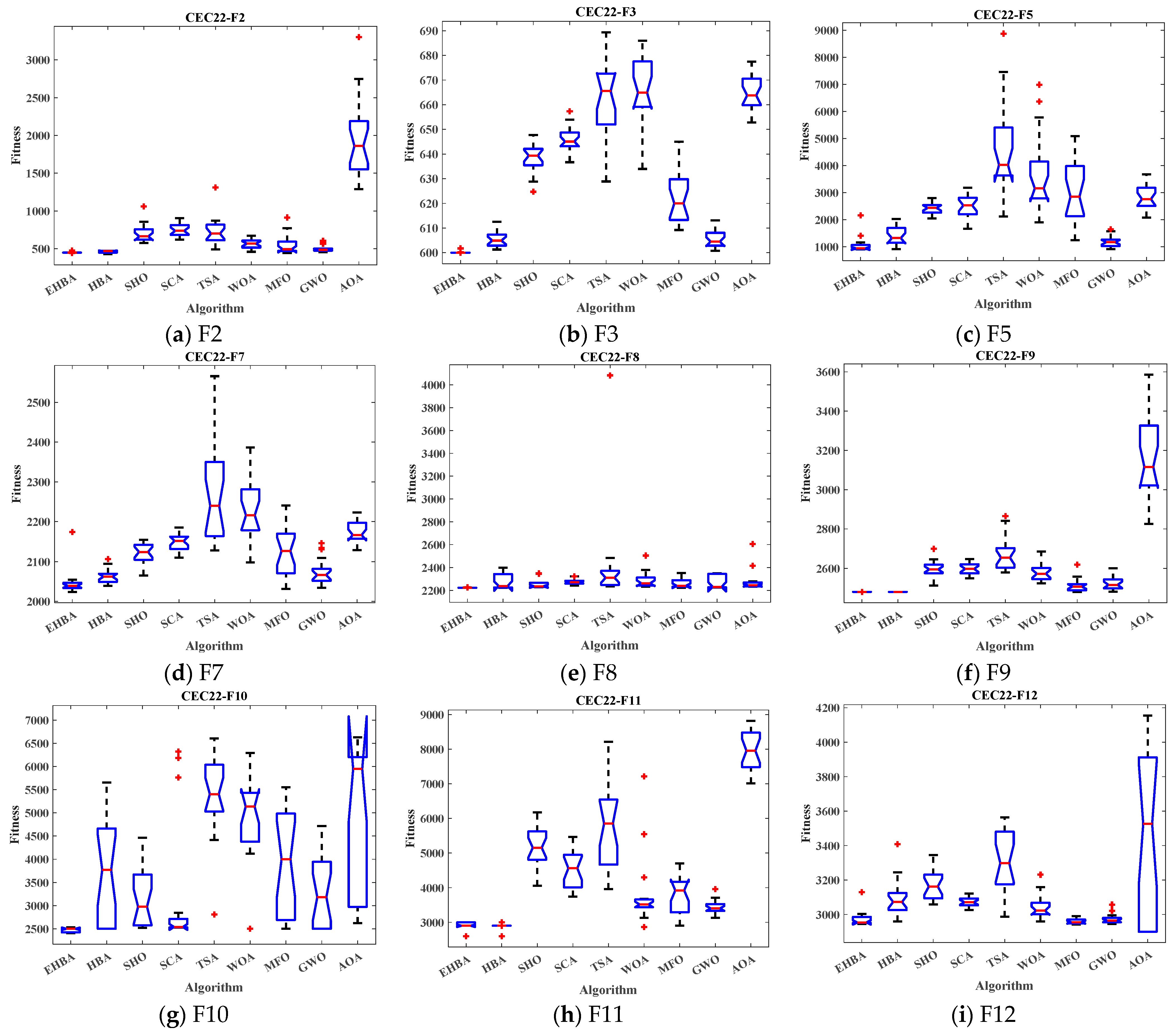
4.3. Experiment and Analysis on the CEC2022 Test Set
5. The Application of EHBA in Engineering Design Issues
5.1. Welding Beam Design Issues
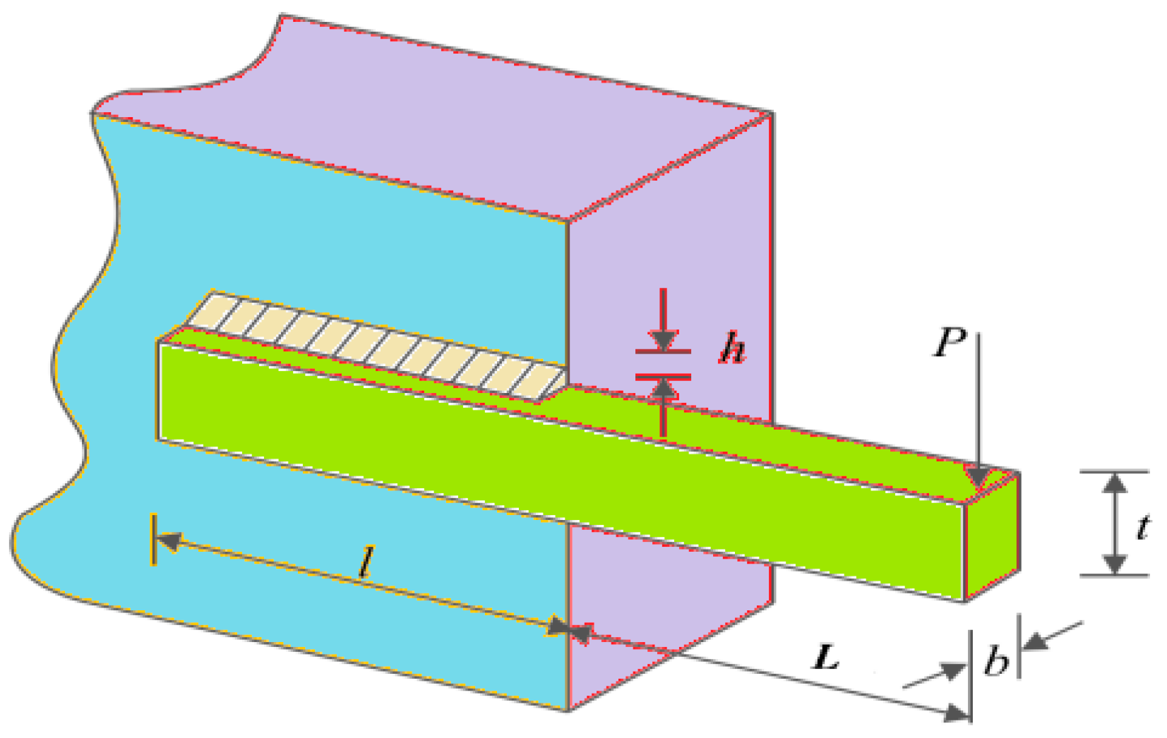
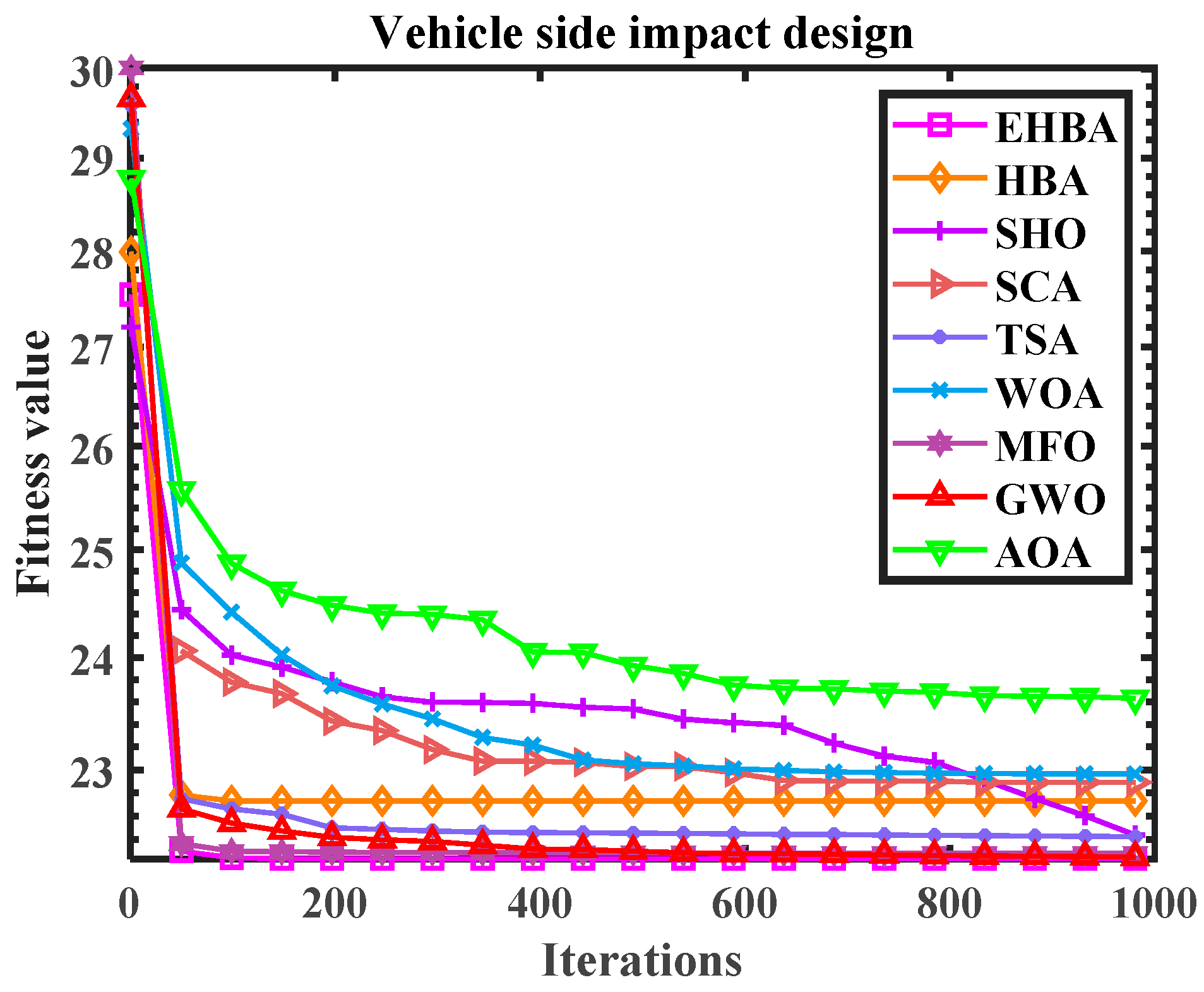
5.2. Vehicle Side Impact Design Issues
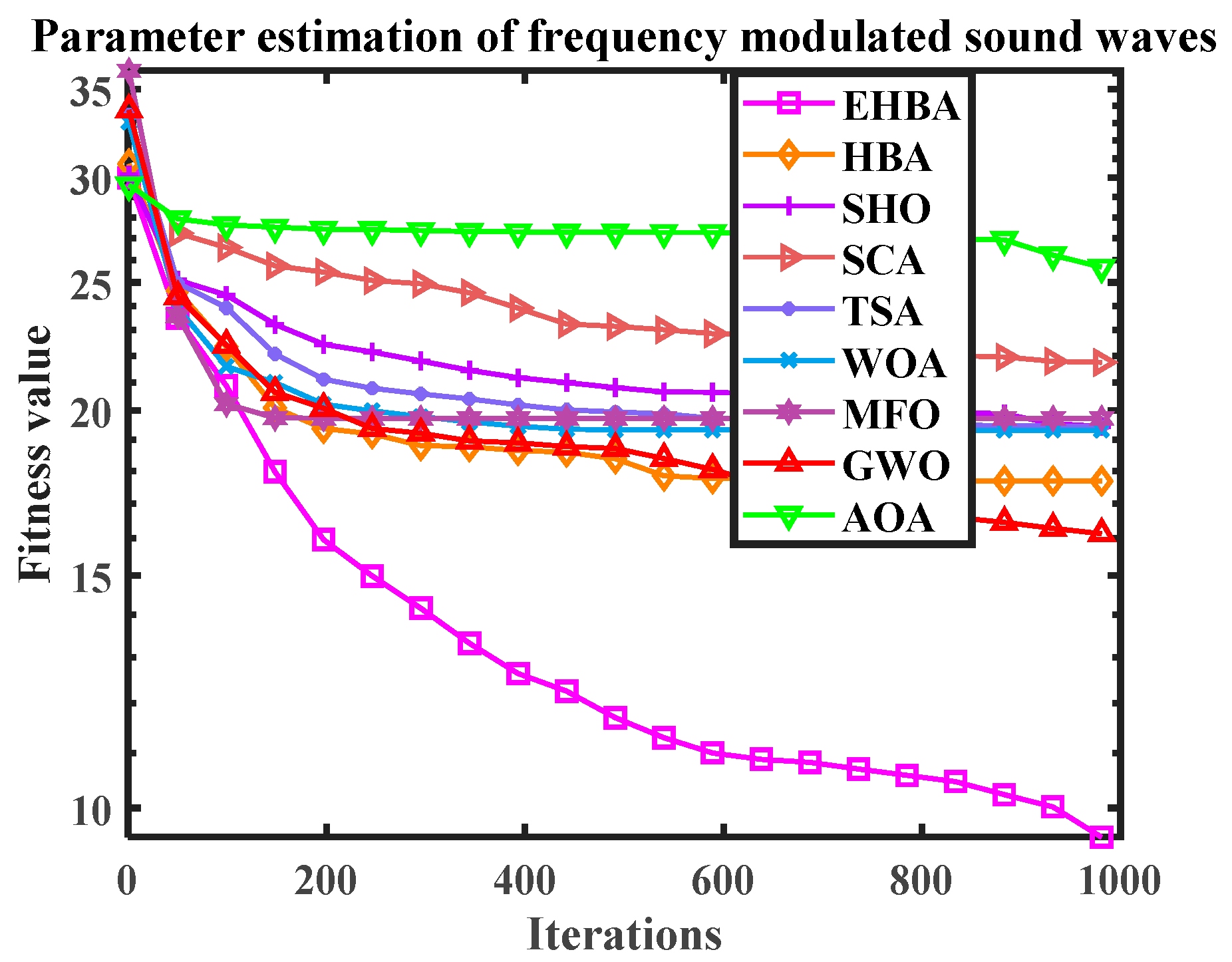
5.3. Parameter Estimation of Frequency Modulated (FM) Sound Waves
6. Conclusions and Future Research
Author Contributions
Funding
Institutional Review Board Statement
Informed Consent Statement
Data Availability Statement
Conflicts of Interest
References
- Jia, H.M.; Li, Y.; Sun, K.J. Simultaneous feature selection optimization based on hybrid sooty tern optimization algorithm and genetic algorithm. Acta Autom. Sin. 2022, 48, 15. [Google Scholar] [CrossRef]
- Jia, H.M.; Jiang, Z.C.; Li, Y. Simultaneous feature selection optimization based on improved bald eagle search algorithm. Control Decis. 2022, 37, 3. [Google Scholar] [CrossRef]
- Jia, H.M.; Jiang, Z.C.; Peng, X.X. Multi-threshold color image segmentation based on improved spotted hyena optimizer. Comput. Appl. Soft. 2020, 37, 261–267. [Google Scholar]
- Zhang, F.Z.; He, Y.Z.; Liu, X.J.; Wang, Z.K. A novel discrete differential evolution algorithm for solving D{0-1} KP problem. J. Front. Comput. Sci. Technol. 2022, 16, 12. [Google Scholar]
- Holland, J.H. Genetic algorithms. Sci. Am. 1992, 267, 66–73. [Google Scholar] [CrossRef]
- Rashedi, E.; Nezamabadi-Pour, H.; Saryazdi, S. GSA: A gravitational search algorithm. Inf. Sci. 2009, 179, 2232–2248. [Google Scholar] [CrossRef]
- Mirjalili, S.; Mirjalili, S.M.; Hatamlou, A. Multi-verse optimizer: A nature-inspired algorithm for global optimization. Neural Comput. Appl. 2016, 27, 495–513. [Google Scholar] [CrossRef]
- Faramarzi, A.; Heidarinejad, M.; Stephens, B.E.; Mirjalili, S. Equilibrium optimizer: A novel optimization algorithm. Knowl.-Based Syst. 2020, 191, 105190. [Google Scholar] [CrossRef]
- Rao, R.V.; Savsani, V.J.; Vakharia, D.P. Teaching-learning-based optimization: An optimization method for continuous non-linear large scale problems. Inf. Sci. 2012, 183, 1–15. [Google Scholar] [CrossRef]
- Moghdani, R.; Salimifard, K. Volleyball premier league algorithm. Appl. Soft Comput. 2018, 64, 161–185. [Google Scholar] [CrossRef]
- Abualigah, L.; Yousri, D.; Elaziz, M.A.; Ewees, A.A.; Al-qaness, M.A.A.; Gandomi, A. Aquila Optimizer: A novel meta-heuristic optimization algorithm. Comput. Ind. Eng. 2021, 157, 107250. [Google Scholar] [CrossRef]
- Lin, S.J.; Dong, C.; Chen, M.Z.; Zhang, F.; Chen, J.H. Summary of new group intelligent optimization algorithms. Comput. Eng. Appl. 2018, 54, 1–9. [Google Scholar] [CrossRef]
- Feng, W.T.; Song, K.K. An Enhanced Whale Optimization Algorithm. Comput. Simul. 2020, 37, 275–279, 357. [Google Scholar] [CrossRef]
- Chen, Y.; Chen, S. Research on Application of Dynamic Weighted Bat Algorithm in Image Segmentation. Comput. Eng. Appl. 2020, 56, 207–215. [Google Scholar] [CrossRef]
- Xue, B.; Zhang, M.; Browne, W.N.; Yao, X. A survey on evolutionary computation approaches to feature selection. IEEE Trans. Evol. Comput. 2016, 20, 606–626. [Google Scholar] [CrossRef]
- Gong, G.; Chiong, R.; Deng, Q.; Gong, X. A hybrid artificial bee colony algorithm for flexible job shop scheduling with worker flexibility. Int. J. Prod. Res. 2019, 58, 4406–4420. [Google Scholar] [CrossRef]
- Tharwat, A.; Elhoseny, M.; Hassanien, A.E.; Gabel, T.; Kumar, A. Intelligent Bézier curve-based path planning model using Chaotic Particle Swarm Optimization algorithm. Clust. Comput. 2019, 22 (Suppl. S2), 4745–4766. [Google Scholar] [CrossRef]
- Askarzadeh, A.; Rezazadeh, A. Artificial neural network training using a new efficient optimization algorithm. Appl. Soft Comput. 2013, 13, 1206–1213. [Google Scholar] [CrossRef]
- Irmak, B.; Karakoyun, M.; Gülcü, Ş. An improved butterfly optimization algorithm for training the feed-forward artificial neural networks. Soft Comput. 2023, 27, 3887–3905. [Google Scholar] [CrossRef]
- Ang, K.M.; Chow, C.E.; El-Kenawy, E.-S.M.; Abdelhamid, A.A.; Ibrahim, A.; Karim, F.K.; Khafaga, D.S.; Tiang, S.S.; Lim, W.H. A Modified Particle Swarm Optimization Algorithm for Optimizing Artificial Neural Network in Classification Tasks. Processes 2022, 10, 2579. [Google Scholar] [CrossRef]
- Ang, K.M.; Lim, W.H.; Tiang, S.S.; Ang, C.K.; Natarajan, E.; Ahamed Khan, M.K.A. Optimal Training of Feedforward Neural Networks Using Teaching-Learning-Based Optimization with Modified Learning Phases. In Proceedings of the 12th National Technical Seminar on Unmanned System Technology 2020. Lecture Notes in Electrical Engineering; Springer: Singapore, 2022; Volume 770. [Google Scholar] [CrossRef]
- Wolpert, D.H.; Macready, W.G. No free lunch theorems for optimization. IEEE Trans. Evol. Comput. 1997, 1, 67–82. [Google Scholar] [CrossRef]
- Eberhart, R.; Kennedy, J. Particle swarm optimization. In Proceedings of the IEEE International Conference on Neural Networks, Perth, Australia, 27 November–1 December 1995; IEEE: Piscataway, NJ, USA, 1995; Volume 4, pp. 1942–1948. [Google Scholar] [CrossRef]
- Dorigo, M.; Maniezzo, V.; Colorni, A. Ant system: Optimization by a colony of cooperating agents. IEEE Trans. Syst. Man Cybern. B 1996, 26, 29–41. [Google Scholar] [CrossRef] [PubMed]
- Yang, X.S.; Gandomi, A.H. Bat algorithm: A novel approach for global engineering optimization. Eng. Comput. 2012, 29, 464–483. [Google Scholar] [CrossRef]
- Gandomi, A.H.; Yang, X.; Alavi, A.H. Cuckoo search algorithm: A metaheuristic approach to solve structural optimization problems. Eng. Comput. 2013, 29, 17–35. [Google Scholar] [CrossRef]
- Mirjalili, S.; Mirjalili, S.M.; Lewis, A. Grey wolf optimizer. Adv. Eng. Softw. 2014, 69, 46–61. [Google Scholar] [CrossRef]
- Mirjalili, S.; Lewis, A. The whale optimization algorithm. Adv. Eng. Softw. 2016, 95, 51–67. [Google Scholar] [CrossRef]
- Mirjalili, S.; Gandomi, A.H.; Mirjalili, S.Z.; Saremi, S.; Faris, H.; Mirjalili, S.M. Salp swarm algorithm: A bio-inspired optimizer for engineering design problems. Adv. Eng. Softw. 2017, 114, 163–191. [Google Scholar] [CrossRef]
- Zhao, S.; Zhang, T.; Ma, S.; Wang, M. Sea-horse optimizer: A novel nature-inspired meta-heuristic for global optimization problems. Appl. Intell. 2022, 53, 11833–11860. [Google Scholar] [CrossRef]
- Abualigah, L.; Elaziz, M.A.; Sumari, P.; Geem, Z.W.; Gandomi, A.H. Reptile Search Algorithm (RSA): A nature-inspired meta-heuristic optimizer. Expert Syst. Appl. 2022, 191, 116158. [Google Scholar] [CrossRef]
- Mirjalili, S. SCA: A sine cosine algorithm for solving optimization problems. Knowl.-Based Syst. 2015, 96, 120–133. [Google Scholar] [CrossRef]
- Kaur, S.; Awasthi, L.K.; Sangal, A.L.; Dhiman, G. Tunicate swarm algorithm: A new bio-inspired based metaheuristic paradigm for global optimization. Eng. Appl. Artif. Intel. 2020, 90, 103541. [Google Scholar] [CrossRef]
- Naruei, I.; Keynia, F. Wild horse optimizer: A new meta-heuristic algorithm for solving engineering optimization problems. Eng. Comput. 2021, 38, 3025–3056. [Google Scholar] [CrossRef]
- Hashim, F.A.; Hussain, K.; Houssein, E.H.; Mabrouk, M.S.; Al-Atabany, W. Archimedes optimization algorithm: A new metaheuristic algorithm for solving optimization problems. Appl. Intell. 2021, 51, 1531–1551. [Google Scholar] [CrossRef]
- Mirjalili, S. Moth-flame optimization algorithm: A novel nature-inspired heuristic paradigm. Knowl.-Based Syst. 2015, 89, 228–249. [Google Scholar] [CrossRef]
- Hashim, F.A.; Houssein, E.H.; Hussain, K.; Mabrouk, M.S.; Al-Atabany, W. Honey badger algorithm: New metaheuristic algorithm for solving optimization problems. Math. Comput. Simulat. 2021, 192, 84–110. [Google Scholar] [CrossRef]
- Akdağ, O. A Developed Honey Badger Optimization Algorithm for Tackling Optimal Power Flow Problem. Electr. Power Compon. Syst. 2022, 50, 331–348. [Google Scholar] [CrossRef]
- Han, E.; Ghadimi, N. Model identification of proton-exchange membrane fuel cells based on a hybrid convolutional neural network and extreme learning machine optimized by improved honey badger algorithm. Sustain. Energy Technol. Assess. 2022, 52, 102005. [Google Scholar] [CrossRef]
- Zhong, J.Y.; Yuan, X.G.; Du, B.; Hu, G.; Zhao, C.Y. An Lévy Flight Based Honey Badger Algorithm for Robot Gripper Problem. In Proceedings of the 7th International Conference on Image, Vision and Computing (ICIVC), Xi’an, China, 26–28 July 2022; pp. 901–905. [Google Scholar] [CrossRef]
- Hu, G.; Zhong, J.Y.; Wei, G. SaCHBA_PDN: Modified honey badger algorithm with multi-strategy for UAV path planning. Expert Syst. Appl. 2023, 223, 119941. [Google Scholar] [CrossRef]
- Kapner, D.; Cook, T.; Adelberger, E.; Gundlach, J.; Heckel, B.R.; Hoyle, C.; Swanson, H. Tests of the gravitational inverse-square law below the dark-energy length scale. Phys. Rev. Lett. 2007, 98, 021101. [Google Scholar] [CrossRef]
- Jia, H.M.; Liu, Q.G.; Liu, Y.X.; Wang, S.; Wu, D. Hybrid Aquila and Harris hawks optimization algorithm with dynamic opposition-based learning. CAAI Trans. Intell. Syst. 2023, 18, 104–116. [Google Scholar] [CrossRef]
- Hua, Y.; Sui, X.; Zhou, S.; Chen, Q.; Gu, G.; Bai, H.; Li, W. A novel method of global optimization for wavefront shaping based on the differential evolution algorithm. Opt. Commun. 2021, 481, 126541. [Google Scholar] [CrossRef]
- Li, X.; Wang, L.; Jiang, Q.; Li, N. Differential evolution algorithm with multi-population cooperation and multi-strategy integration. Neurocomputing 2021, 421, 285–302. [Google Scholar] [CrossRef]
- Cheng, J.; Pan, Z.; Liang, H.; Gao, Z.; Gao, J. Differential evolution algorithm with fitness and diversity ranking-based mutation operator. Swarm Evol. Comput. 2021, 61, 100816. [Google Scholar] [CrossRef]
- Xu, C.H.; Luo, Z.H.; Wu, G.H.; Liu, B. Grey wolf optimization algorithm based on sine factor and quantum local search. Comput. Eng. Appl. 2021, 57, 83–89. [Google Scholar] [CrossRef]
- Deep, K.; Bansal, J.C. Optimization of directional over current relay times using Laplace Crossover Particle Swarm Optimization (LXPSO). In Proceedings of the 2009 World Congress on Nature & Biologically Inspired Computing (NaBIC), Coimbatore, India, 9–11 December 2009; pp. 288–293. [Google Scholar] [CrossRef]
- Wan, Y.G.; Li, X.; Guan, L.Z. Improved Whale Optimization Algorithm for Solving High-dimensional Optimization Problems. J. Front. Comput. Sci. Technol. 2021, 112, 107854. [Google Scholar]
- Awad, N.H.; Ali, M.Z.; Liang, J.J.; Qu, B.Y.; Suganthan, P.N. Problem Definitions and Evaluation Criteria for the CEC2017 Special Session and Competition on Single Objective Bound Constrained Real-Parameter Numerical Optimization; Technical Report; Nanyang Technological University: Singapore, 2016. [Google Scholar]
- Yue, C.T.; Price, K.V.; Suganthan, P.N.; Liang, J.J.; Ali, M.Z.; Qu, B.Y.; Awad, N.H.; Biswas, P.P. Problem Definitions and Evaluation Criteria for the CEC2020 Special Session and Competition on Single Objective Bound Constrained Numerical Optimization; Technical Report; Computational Intelligence Laboratory, Zhengzhou University, Zhengzhou China and Technical Report; Nanyang Technological University: Singapore; Glasgow, UK, 2020. [Google Scholar]
- Yazdani, D.; Branke, J.; Omidvar, M.N.; Li, X.; Li, C.; Mavrovouniotis, M.; Nguyen, T.T.; Yang, S.; Yao, X. IEEE CEC 2022 Competition on Dynamic Optimization Problems Generated by Generalized Moving Peaks Benchmark. arXiv 2021, arXiv:2106.06174. [Google Scholar] [CrossRef]
- Wu, L.H.; Wang, Y.N.; Zhou, S.W.; Yuan, X.F. Differential evolution for nonlinear constrained optimization using non-stationary multi-stage assignment penalty function. Syst. Eng. Theory Pract. 2007, 27, 128–133. [Google Scholar] [CrossRef]
- Youn, B.D.; Choi, K.K.; Yang, R.J.; Gu, L. Reliability-based design optimization for crash worthiness of vehicle side impact. Struct. Multidiscip. Optim. 2004, 26, 272–283. [Google Scholar] [CrossRef]
- Gothania, B.; Mathur, G.; Yadav, R.P. Accelerated artificial bee colony algorithm for parameter estimation of frequency-modulated sound waves. Int. J. Electron. Commun. Eng. 2014, 7, 63–74. [Google Scholar]
- Hu, G.; Du, B.; Wang, X.F.; Wei, G. An enhanced black widow optimization algorithm for feature selection. Knowl.-Based Syst. 2022, 235, 107638. [Google Scholar] [CrossRef]
- Zheng, J.; Ji, X.; Ma, Z.; Hu, G. Construction of Local-Shape-Controlled Quartic Generalized Said-Ball Model. Mathematics 2023, 11, 2369. [Google Scholar] [CrossRef]
- Hu, G.; Guo, Y.X.; Wei, G.; Abualigah, L. Genghis Khan shark optimizer: A novel nature-inspired algorithm for engineering optimization. Adv. Eng. Inform. 2023, 58, 102210. [Google Scholar] [CrossRef]
- Hu, G.; Zheng, Y.X.; Abualigah, L.; Hussien, A.G. DETDO: An adaptive hybrid dandelion optimizer for engineering optimization. Adv. Eng. Inform. 2023, 57, 102004. [Google Scholar] [CrossRef]


| Algorithms | Parameters | Setting Value |
|---|---|---|
| HBA, EHBA | Coefficient of the logarithmic spiral shape β (the ability of a honey badger to get food) | 6 |
| C | 2 | |
| SHO | Logarithmic helix constant | u = 0.05, v = 0.05 |
| Constant parameters l | l = 0.05 | |
| AOA | Constant parameters | c1 = 2, c2 = 6, c3 = 1, c4 = 2 |
| WOA | Control parameter a Constant parameters b | a is linear decrease from 2 to 0 b = 1 |
| MFO | Shape constant of logarithmic spiral b | b = 1 |
| TSA | Initial interaction velocity constant Pmin, Pmax | Pmin = 1, Pmax = 4 |
| SCA | Constant parameters a | a = 2 |
| GWO | Control parameter a | a is linear decrease from 2 to 0 |
| F | Index | Algorithms | ||||||||
|---|---|---|---|---|---|---|---|---|---|---|
| EHBA | HBA | SHO | SCA | TSA | WOA | MFO | GWO | AOA | ||
| F1 | Ave | 6.940 × 10³ | 2.116 × 10⁴ | 2.036 × 10¹⁰ | 1.776 × 10¹⁰ | 2.043 × 10¹⁰ | 1.875 × 10⁹ | 1.044 × 10¹⁰ | 2.469 × 10⁹ | 5.208 × 10¹⁰ |
| Std | 6.075 × 10³ | 5.366 × 10⁴ | 6.035 × 10⁹ | 2.884 × 10⁹ | 5.480 × 10⁹ | 1.367 × 10⁹ | 8.340 × 10⁹ | 1.791 × 10⁹ | 7.679 × 10⁹ | |
| Best | 4.300 × 10² | 9.124 × 10² | 6.912 × 10⁹ | 1.246 × 10¹⁰ | 6.148 × 10⁹ | 6.860 × 10⁸ | 1.824 × 10⁹ | 7.948 × 10⁸ | 4.107 × 10¹⁰ | |
| Rank | 1 | 2 | 7 | 6 | 8 | 3 | 5 | 4 | 9 | |
| F3 | Ave | 2.908 × 10⁴ | 1.885 × 10⁴ | 6.359 × 10⁴ | 6.253 × 10⁴ | 4.720 × 10⁴ | 2.536 × 10⁵ | 1.388 × 10⁵ | 5.102 × 10⁴ | 5.539 × 10⁴ |
| Std | 6.627 × 10³ | 5.071 × 10³ | 9.618 × 10³ | 1.100 × 10⁴ | 9.274 × 10³ | 7.388 × 10⁴ | 6.077 × 10⁴ | 1.381 × 10⁴ | 9.598 × 10³ | |
| Best | 1.723 × 10⁴ | 1.077 × 10⁴ | 4.048 × 10⁴ | 4.732 × 10⁴ | 2.599 × 10⁴ | 1.688 × 10⁵ | 4.195 × 10⁴ | 1.461 × 10⁴ | 3.291 × 10⁴ | |
| Rank | 2 | 1 | 7 | 6 | 3 | 9 | 8 | 4 | 5 | |
| F4 | Ave | 5.049 × 10² | 5.151 × 10² | 3.487 × 10³ | 2.466 × 10³ | 3.914 × 10³ | 8.298 × 10² | 1.263 × 10³ | 6.419 × 10² | 1.096 × 10⁴ |
| Std | 3.796 × 101 | 2.728 × 101 | 1.636 × 10³ | 8.131 × 10² | 2.526 × 10³ | 1.009 × 10² | 9.391 × 10² | 1.665 × 10² | 2.162 × 10³ | |
| Best | 4.046 × 10² | 4.733 × 10² | 1.118 × 10³ | 1.545 × 10³ | 8.272 × 10² | 5.865 × 10² | 5.877 × 10² | 5.272 × 10² | 7.314 × 10³ | |
| Rank | 1 | 2 | 7 | 6 | 8 | 4 | 5 | 3 | 9 | |
| F5 | Ave | 6.103 × 10² | 6.216 × 10² | 7.268 × 10² | 8.185 × 10² | 8.335 × 10² | 8.309 × 10² | 7.045 × 10² | 6.204 × 10² | 8.680 × 10² |
| Std | 1.664 × 101 | 2.609 × 101 | 2.710 × 101 | 2.758 × 101 | 4.902 × 101 | 5.581 × 101 | 3.487 × 101 | 4.249 × 101 | 2.702 × 101 | |
| Best | 5.853 × 10² | 5.657 × 10² | 6.912 × 10² | 7.852 × 10² | 7.145 × 10² | 6.699 × 10² | 6.440 × 10² | 5.659 × 10² | 8.008 × 10² | |
| Rank | 1 | 3 | 5 | 6 | 8 | 7 | 4 | 2 | 9 | |
| F6 | Ave | 6.002 × 10² | 6.141 × 10² | 6.485 × 10² | 6.581 × 10² | 6.833 × 10² | 6.801 × 10² | 6.428 × 10² | 6.104 × 10² | 6.768 × 10² |
| Std | 2.683 × 10⁻¹ | 6.140 × 100 | 6.153 × 100 | 6.172 × 100 | 1.378 × 101 | 1.205 × 101 | 1.368 × 101 | 4.147 × 100 | 4.811 × 100 | |
| Best | 6.000 × 10² | 6.066 × 10² | 6.352 × 10² | 6.455 × 10² | 6.597 × 10² | 6.537 × 10² | 6.194 × 10² | 6.018 × 10² | 6.682 × 10² | |
| Rank | 1 | 3 | 5 | 6 | 9 | 8 | 4 | 2 | 7 | |
| F7 | Ave | 8.715 × 10² | 9.302 × 10² | 1.131 × 10³ | 1.202 × 10³ | 1.258 × 10³ | 1.256 × 10³ | 1.052 × 10³ | 9.302 × 10² | 1.362 × 10³ |
| Std | 3.822 × 101 | 5.782 × 101 | 5.359 × 101 | 6.706 × 101 | 1.000 × 10² | 1.216 × 10² | 1.466 × 10² | 5.838 × 101 | 5.943 × 101 | |
| Best | 8.130 × 10² | 8.640 × 10² | 1.036 × 10³ | 1.090 × 10³ | 1.132 × 10³ | 1.048 × 10³ | 8.339 × 10² | 8.459 × 10² | 1.243 × 10³ | |
| Rank | 1 | 3 | 5 | 6 | 8 | 7 | 4 | 2 | 9 | |
| F8 | Ave | 8.985 × 10² | 9.036 × 10² | 9.781 × 10² | 1.081 × 10³ | 1.111 × 10³ | 1.059 × 10³ | 1.016 × 10³ | 8.991 × 10² | 1.100 × 10³ |
| Std | 2.029 × 101 | 2.444 × 101 | 2.901 × 101 | 2.194 × 101 | 5.049 × 101 | 5.459 × 101 | 5.290 × 101 | 2.235 × 101 | 2.551 × 101 | |
| Best | 8.701 × 10² | 8.557 × 10² | 9.206 × 10² | 1.040 × 10³ | 1.031 × 10³ | 9.860 × 10² | 9.466 × 10² | 8.705 × 10² | 1.049 × 10³ | |
| Rank | 1 | 3 | 4 | 7 | 9 | 6 | 5 | 2 | 8 | |
| F9 | Ave | 1.235 × 10² | 3.043 × 10³ | 5.260 × 10³ | 7.498 × 10³ | 1.105 × 10⁴ | 1.007 × 10⁴ | 6.909 × 10³ | 2.599 × 10³ | 9.035 × 10³ |
| Std | 4.100 × 10² | 9.862 × 10² | 8.810 × 10² | 1.349 × 10³ | 3.400 × 10³ | 3.877 × 10³ | 1.678 × 10³ | 1.874 × 10³ | 9.305 × 10² | |
| Best | 9.054 × 10² | 1.623 × 10³ | 3.284 × 10³ | 5.246 × 10³ | 5.192 × 10³ | 6.380 × 10³ | 3.775 × 10³ | 1.175 × 10³ | 6.816 × 10³ | |
| Rank | 1 | 3 | 4 | 6 | 9 | 8 | 5 | 2 | 7 | |
| F10 | Ave | 4.970 × 10³ | 5.513 × 10³ | 5.693 × 10³ | 8.736 × 10³ | 7.183 × 10³ | 7.257 × 10³ | 5.657 × 10³ | 4.575 × 10³ | 8.405 × 10³ |
| Std | 6.279 × 10² | 1.498 × 10³ | 5.170 × 10² | 2.679 × 10² | 6.318 × 10² | 8.110 × 10² | 6.857 × 10² | 9.121 × 10² | 3.467 × 10² | |
| Best | 2.817 × 10³ | 3.856 × 10³ | 4.769 × 10³ | 8.208 × 10³ | 5.945 × 10³ | 5.750 × 10³ | 4.122 × 10³ | 3.673 × 10³ | 7.486 × 10³ | |
| Rank | 2 | 3 | 5 | 9 | 6 | 7 | 4 | 1 | 8 | |
| F11 | Ave | 1.201 × 10³ | 1.274 × 10³ | 3.282 × 10³ | 3.080 × 10³ | 5.717 × 10³ | 6.606 × 10³ | 4.853 × 10³ | 2.233 × 10³ | 7.360 × 10³ |
| Std | 3.024 × 101 | 5.679 × 101 | 1.494 × 10³ | 7.678 × 10² | 2.695 × 10³ | 3.322 × 10³ | 8.710 × 10³ | 9.032 × 10² | 1.705 × 10³ | |
| Best | 1.132 × 10³ | 1.187 × 10³ | 1.620 × 10³ | 1.977 × 10³ | 1.772 × 10³ | 2.088 × 10³ | 1.375 × 10³ | 1.275 × 10³ | 3.978 × 10³ | |
| Rank | 1 | 2 | 5 | 4 | 7 | 8 | 6 | 3 | 9 | |
| F12 | Ave | 1.169 × 10⁷ | 1.096 × 10⁷ | 1.983 × 10¹⁰ | 1.762 × 10¹⁰ | 2.455 × 10¹⁰ | 1.623 × 10⁹ | 7.032 × 10⁹ | 1.186 × 10⁹ | 6.502 × 10¹⁰ |
| Std | 6.141 × 10⁶ | 9.818 × 10⁶ | 7.132 × 10⁹ | 3.949 × 10⁹ | 1.384 × 10¹⁰ | 5.255 × 10⁸ | 5.918 × 10⁹ | 1.111 × 10⁹ | 9.469 × 10⁹ | |
| Best | 3.678 × 10⁶ | 3.699 × 10⁶ | 8.820 × 10⁹ | 1.406 × 10¹⁰ | 8.337 × 10⁹ | 6.302 × 10⁸ | 1.132 × 10⁹ | 1.201 × 10⁸ | 5.259 × 10¹⁰ | |
| Rank | 2 | 1 | 7 | 6 | 8 | 4 | 5 | 3 | 9 | |
| F13 | Ave | 2.862 × 10⁴ | 4.082× 10⁴ | 4.596 × 10⁸ | 8.223 × 10⁸ | 3.208 × 10⁹ | 2.150 × 10⁶ | 7.182 × 10⁷ | 1.436 × 10⁷ | 5.248 × 10⁹ |
| Std | 6.761 × 10⁴ | 3.591× 10⁴ | 1.181 × 10⁹ | 2.120 × 10⁸ | 4.547 × 10⁹ | 2.336 × 10⁶ | 3.031 × 10⁸ | 3.725 × 10⁷ | 1.977 × 10⁹ | |
| Best | 2.462 × 10³ | 7.882 × 10³ | 8.005 × 10⁵ | 5.302 × 10⁸ | 4.076 × 10⁷ | 2.296 × 10⁵ | 2.883 × 10⁴ | 2.902 × 10⁴ | 1.371 × 10⁹ | |
| Rank | 1 | 2 | 6 | 7 | 8 | 3 | 5 | 4 | 9 | |
| F14 | Ave | 4.670 × 10⁵ | 9.018 × 10⁵ | 7.040 × 10⁶ | 7.230 × 10⁶ | 2.527 × 10⁷ | 4.218 × 10⁶ | 4.315 × 10⁶ | 1.368 × 10⁶ | 1.196 × 10⁸ |
| Std | 2.301 × 10⁵ | 2.423 × 10⁶ | 5.367 × 10⁶ | 5.031 × 10⁶ | 4.207 × 10⁷ | 2.794 × 10⁶ | 4.907 × 10⁶ | 1.205 × 10⁶ | 5.024 × 10⁷ | |
| Best | 1.379 × 10⁵ | 4.415 × 10⁴ | 1.256 × 10⁶ | 1.709 × 10⁶ | 6.223 × 10⁵ | 2.136 × 10⁵ | 1.560 × 10⁵ | 1.082 × 10⁵ | 3.903 × 10⁷ | |
| Rank | 1 | 2 | 6 | 7 | 8 | 4 | 5 | 3 | 9 | |
| F15 | Ave | 1.124 × 10⁴ | 1.65 × 10⁴ | 2.910 × 10⁵ | 3.238 × 10⁷ | 1.373 × 10⁸ | 3.773 × 10⁶ | 4.010 × 10⁴ | 3.399 × 10⁶ | 2.103 × 10⁸ |
| Std | 1.343 × 10⁴ | 1.406 × 10⁴ | 5.303 × 10⁵ | 2.574 × 10⁷ | 2.274 × 10⁸ | 6.591 × 10⁶ | 2.966 × 10⁴ | 1.466 × 10⁷ | 2.340 × 10⁸ | |
| Best | 1.836 × 10³ | 3.024 × 10³ | 1.386 × 10⁶ | 1.754 × 10⁶ | 9.574 × 10⁴ | 1.417 × 10⁵ | 6.000 × 10³ | 2.200 × 10⁴ | 6.277 × 10⁶ | |
| Rank | 1 | 2 | 4 | 7 | 8 | 6 | 3 | 5 | 9 | |
| F16 | Ave | 2.375 × 10³ | 2.860 × 10³ | 3.054 × 10³ | 3.955 × 10³ | 3.646 × 10³ | 4.286 × 10³ | 3.255 × 10³ | 2.740 × 10³ | 5.506 × 10³ |
| Std | 2.289 × 10² | 4.421 × 10² | 3.268 × 10² | 2.684 × 10² | 6.790 × 10² | 7.032 × 10² | 4.167 × 10² | 4.395 × 10² | 8.078 × 10² | |
| Best | 1.986 × 10³ | 2.026 × 10³ | 2.277 × 10³ | 3.519 × 10³ | 2.767 × 10³ | 3.139 × 10³ | 2.631 × 10³ | 2.047 × 10³ | 4.204 × 10³ | |
| Rank | 1 | 3 | 4 | 7 | 6 | 8 | 5 | 2 | 9 | |
| F17 | Ave | 1.944 × 10³ | 2.214 × 10³ | 2.408 × 10³ | 2.672 × 10³ | 2.595 × 10³ | 2.808 × 10³ | 2.602 × 10³ | 2.018 × 10³ | 3.334 × 10³ |
| Std | 1.504 × 10² | 2.166 × 10² | 2.663 × 10² | 1.522 × 10² | 3.417 × 10² | 2.243 × 10² | 3.607 × 10² | 1.093 × 10² | 4.563 × 10² | |
| Best | 1.759 × 10³ | 1.859 × 10³ | 1.886 × 10³ | 2.432 × 10³ | 2.043 × 10³ | 2.439 × 10³ | 1.957 × 10³ | 1.832 × 10³ | 2.615 × 10³ | |
| Rank | 1 | 3 | 4 | 7 | 5 | 8 | 6 | 2 | 9 | |
| F18 | Ave | 1.572 × 10⁶ | 1.701 × 10⁶ | 1.457 × 10⁷ | 3.276 × 10⁷ | 2.070 × 10⁷ | 4.441 × 10⁷ | 1.377 × 10⁷ | 8.983 × 10⁶ | 1.157 × 10⁸ |
| Std | 1.083 × 10⁶ | 1.540 × 10⁶ | 1.733 × 10⁷ | 1.154 × 10⁷ | 2.021 × 10⁷ | 2.813 × 10⁷ | 1.061 × 10⁷ | 1.183 × 10⁷ | 3.164 × 10⁷ | |
| Best | 2.608 × 10⁵ | 2.711 × 10⁵ | 4.623 × 10⁶ | 1.346 × 10⁷ | 1.374 × 10⁶ | 1.894 × 10⁷ | 1.344 × 10⁶ | 7.288 × 10⁵ | 5.250 × 10⁷ | |
| Rank | 1 | 2 | 5 | 7 | 6 | 8 | 4 | 3 | 9 | |
| F19 | Ave | 6.171 × 10³ | 1.205 × 10⁴ | 1.056 × 10⁷ | 5.981 × 10⁷ | 3.992 × 10⁸ | 1.648 × 10⁷ | 6.896 × 10⁷ | 1.677 × 10⁶ | 5.337 × 10⁸ |
| Std | 5.556 × 10³ | 1.457 × 10⁴ | 3.343 × 10⁷ | 3.563 × 10⁷ | 9.671 × 10⁸ | 1.085 × 10⁷ | 2.969 × 10⁸ | 2.021 × 10⁶ | 3.838 × 10⁸ | |
| Best | Best | 1.936 × 10³ | 2.162 × 10³ | 1.021 × 10⁴ | 1.918 × 10⁷ | 1.582 × 10⁵ | 5.604 × 10⁵ | 1.109 × 10⁴ | 8.336 × 10³ | 1.025 × 10⁷ |
| Rank | 1 | 2 | 4 | 6 | 8 | 5 | 7 | 3 | 9 | |
| F20 | Ave | 2.240 × 10³ | 2.547 × 10³ | 2.638 × 10³ | 2.865 × 10³ | 2.808 × 10³ | 2.853 × 10³ | 2.750 × 10³ | 2.421 × 10³ | 2.868 × 10³ |
| Std | 1.131 × 10² | 2.447 × 10² | 2.019 × 10² | 1.332 × 10² | 2.107 × 10² | 2.034 × 10² | 2.176 × 10² | 1.364 × 10² | 1.370 × 10² | |
| Best | 2.149 × 10³ | 2.222 × 10³ | 2.305 × 10³ | 2.601 × 10³ | 2.460 × 10³ | 2.451 × 10³ | 2.320 × 10³ | 2.171 × 10³ | 2.568 × 10³ | |
| Rank | 1 | 3 | 4 | 8 | 6 | 7 | 5 | 2 | 9 | |
| F21 | Ave | 2.401 × 10³ | 2.406 × 10³ | 2.503 × 10³ | 2.591 × 10³ | 2.650 × 10³ | 2.619 × 10³ | 2.498 × 10³ | 2.415 × 10³ | 2.628 × 10³ |
| Std | 2.010 × 101 | 3.290 × 101 | 2.864 × 101 | 2.077 × 101 | 4.877 × 101 | 6.677 × 101 | 5.385 × 101 | 4.413 × 101 | 2.389 × 101 | |
| Best | 2.365 × 10³ | 2.347 × 10³ | 2.455 × 10³ | 2.554 × 10³ | 2.556 × 10³ | 2.538 × 10³ | 2.391 × 10³ | 2.360 × 10³ | 2.583 × 10³ | |
| Rank | 1 | 2 | 5 | 6 | 9 | 7 | 4 | 3 | 8 | |
| F22 | Ave | 2.502 × 10³ | 4.053 × 10³ | 6.678 × 10³ | 9.760 × 10³ | 8.438 × 10³ | 7.757 × 10³ | 6.669 × 10³ | 4.752 × 10³ | 9.449 × 10³ |
| Std | 9.030 × 10² | 2.669 × 10³ | 1.420 × 10³ | 1.367 × 10³ | 1.624 × 10³ | 1.927 × 10³ | 7.371 × 10² | 1.762 × 10³ | 8.479 × 10² | |
| Best | 2.300 × 10³ | 2.300 × 10³ | 3.574 × 10³ | 4.487 × 10³ | 3.731 × 10³ | 2.585 × 10³ | 5.660 × 10³ | 2.396 × 10³ | 7.570 × 10³ | |
| Rank | 1 | 2 | 5 | 9 | 7 | 6 | 4 | 3 | 8 | |
| F23 | Ave | 2.754 × 10³ | 2.799 × 10³ | 2.987 × 10³ | 3.073 × 10³ | 3.218 × 10³ | 3.121 × 10³ | 2.829 × 10³ | 2.792 × 10³ | 3.556 × 10³ |
| Std | 2.395 × 101 | 5.438 × 101 | 4.057 × 101 | 3.885 × 101 | 1.546 × 10² | 9.451 × 101 | 3.803 × 101 | 4.361 × 101 | 1.205 × 10² | |
| Best | 2.700 × 10³ | 2.724 × 10³ | 2.918 × 10³ | 3.005 × 10³ | 3.028 × 10³ | 2.989 × 10³ | 2.779 × 10³ | 2.741 × 10³ | 3.297 × 10³ | |
| Rank | 1 | 3 | 5 | 6 | 8 | 7 | 4 | 2 | 9 | |
| F24 | Ave | 2.960 × 10³ | 3.086 × 10³ | 3.300 × 10³ | 3.227 × 10³ | 3.365 × 10³ | 3.229 × 10³ | 2.991 × 10³ | 2.923 × 10³ | 3.772 × 10³ |
| Std | 3.035 × 101 | 1.867 × 10² | 7.077 × 101 | 4.405 × 101 | 1.219 × 10² | 1.025 × 10² | 3.539 × 101 | 3.966 × 101 | 1.888 × 10² | |
| Best | 2.902 × 10³ | 2.851 × 10³ | 3.195 × 10³ | 3.156 × 10³ | 3.158 × 10³ | 3.060 × 10³ | 2.940 × 10³ | 2.867 × 10³ | 3.467 × 10³ | |
| Rank | 2 | 4 | 7 | 5 | 8 | 6 | 3 | 1 | 9 | |
| F25 | Ave | 2.901 × 10³ | 2.905 × 10³ | 3.456 × 10³ | 3.345 × 10³ | 3.593 × 10³ | 3.098 × 10³ | 3.232 × 10³ | 3.015 × 10³ | 4.624 × 10³ |
| Std | 1.828 × 101 | 1.957 × 101 | 2.252 × 10² | 1.121 × 10² | 3.408 × 10² | 5.812 × 101 | 4.286 × 10² | 8.485 × 101 | 4.476 × 10² | |
| Best | 2.884 × 10³ | 2.884 × 10³ | 3.102 × 10³ | 3.196 × 10³ | 3.203 × 10³ | 2.991 × 10³ | 2.888 × 10³ | 2.940 × 10³ | 3.695 × 10³ | |
| Rank | 1 | 2 | 7 | 6 | 8 | 4 | 5 | 3 | 9 | |
| F26 | Ave | 4.555 × 10³ | 4.504 × 10³ | 7.303 × 10³ | 7.551 × 10³ | 8.400 × 10³ | 8.546 × 10³ | 6.068 × 10³ | 4.891 × 10³ | 1.029 × 10⁴ |
| Std | 6.324 × 10² | 1.120 × 10³ | 8.007 × 10² | 3.042 × 10² | 1.726 × 10³ | 9.515 × 10² | 5.199 × 10² | 4.851 × 10² | 6.964 × 10² | |
| Best | 2.800 × 10³ | 2.811 × 10³ | 5.649 × 10³ | 7.043 × 10³ | 3.796 × 10³ | 7.109 × 10³ | 5.081 × 10³ | 4.087 × 10³ | 9.013 × 10³ | |
| Rank | 2 | 1 | 5 | 6 | 7 | 8 | 4 | 3 | 9 | |
| F27 | Ave | 3.231 × 10³ | 3.408 × 10³ | 3.540 × 10³ | 3.514 × 10³ | 3.670 × 10³ | 3.560 × 10³ | 3.261 × 10³ | 3.257 × 10³ | 3.654 × 10³ |
| Std | 2.172 × 101 | 2.140 × 10² | 1.374 × 10² | 8.689 × 101 | 2.326 × 10² | 2.318 × 10² | 2.638 × 101 | 3.699 × 101 | 6.057 × 10² | |
| Best | 3.204 × 10³ | 3.203 × 10³ | 3.368 × 10³ | 3.382 × 10³ | 3.366 × 10³ | 3.293 × 10³ | 3.231 × 10³ | 3.203 × 10³ | 3.200 × 10³ | |
| Rank | 1 | 4 | 6 | 5 | 9 | 7 | 3 | 2 | 8 | |
| F28 | Ave | 3.253 × 10³ | 3.233 × 10³ | 4.160 × 10³ | 4.262 × 10³ | 4.721 × 10³ | 3.544 × 10³ | 3.783 × 10³ | 3.451 × 10³ | 5.352 × 10³ |
| Std | 5.239 × 101 | 2.465 × 101 | 4.107 × 10² | 2.602 × 10² | 5.381 × 10² | 1.141 × 10² | 3.947 × 10² | 1.029 × 10² | 1.571 × 10³ | |
| Best | 3.206 × 10³ | 3.203 × 10³ | 3.590 × 10³ | 3.942 × 10³ | 3.898 × 10³ | 3.403 × 10³ | 3.304 × 10³ | 3.310 × 10³ | 3.300 × 10³ | |
| Rank | 2 | 1 | 6 | 7 | 8 | 4 | 5 | 3 | 9 | |
| F29 | Ave | 3.621 × 10³ | 4.379 × 10³ | 4.350 × 10³ | 5.116 × 10³ | 4.857 × 10³ | 5.207 × 10³ | 4.299 × 10³ | 3.905 × 10³ | 6.297 × 10³ |
| Std | 1.801 × 10² | 8.364 × 10² | 2.871 × 10² | 3.841 × 10² | 4.141 × 10² | 4.619 × 10² | 3.061 × 10² | 2.067 × 10² | 7.947 × 10² | |
| Best | Best | 3.393 × 10³ | 3.643 × 10³ | 3.758 × 10³ | 4.436 × 10³ | 4.251 × 10³ | 4.427 × 10³ | 3.709 × 10³ | 3.655 × 10³ | 4.940 × 10³ |
| Rank | 1 | 5 | 4 | 7 | 6 | 8 | 3 | 2 | 9 | |
| F30 | Ave | 2.703 × 10⁴ | 5.087 × 10⁴ | 8.922 × 10⁶ | 1.603 × 10⁸ | 2.463 × 10⁷ | 3.301 × 10⁷ | 1.178 × 10⁶ | 6.930 × 10⁶ | 1.191 × 10⁹ |
| Std | 1.575 × 10⁴ | 6.900 × 10⁴ | 9.825 × 10⁶ | 8.697 × 10⁷ | 1.589 × 10⁷ | 2.176 × 10⁷ | 2.038 × 10⁶ | 5.327 × 10⁶ | 5.720 × 10⁷ | |
| Best | 8.203 × 10³ | 1.294 × 10⁴ | 1.040 × 10⁶ | 5.523 × 10⁷ | 5.505 × 10⁶ | 5.552 × 10⁶ | 1.917× 10⁴ | 2.344 × 10⁶ | 2.332 × 10⁷ | |
| Rank | 1 | 2 | 5 | 8 | 6 | 7 | 3 | 4 | 9 | |
| Mean Rank | 1.2069 | 2.4483 | 5.2759 | 6.5172 | 7.3793 | 6.3448 | 4.5862 | 2.6897 | 8.5517 | |
| Result | 1 | 2 | 5 | 7 | 8 | 6 | 4 | 3 | 9 | |
| Result | Algorithms | |||||||
|---|---|---|---|---|---|---|---|---|
| HBA | SHO | SCA | TSA | WOA | MFO | GWO | AOA | |
| F1 | 4.09356 × 10⁻¹ | - | - | - | - | - | - | - |
| F3 | 2.30247 × 10⁻⁵ | 7.89803 × 10⁻⁸ | - | 2.06160 × 10⁻⁶ | - | 7.89803 × 10⁻⁸ | 1.10447 × 10⁻⁵ | 1.65708 × 10⁻⁷ |
| F4 | 3.50702 × 10⁻¹ | - | - | - | 7.89803 × 10⁻⁸ | 7.89803 × 10⁻⁸ | 7.94795 × 10⁻⁷ | - |
| F5 | 9.09074 × 10⁻² | - | - | - | - | 7.89803 × 10⁻⁸ | 8.18149 × 10⁻¹ | - |
| F6 | - | - | - | - | - | - | - | - |
| F7 | 5.62904 × 10⁻⁴ | - | - | - | - | 4.16576 × 10⁻⁵ | 1.95335 × 10⁻³ | - |
| F8 | 4.56951 × 10⁻¹ | 1.06457 × 10⁻⁷ | - | - | - | - | 9.67635 × 10⁻¹ | - |
| F9 | 2.95975 × 10⁻⁷ | - | - | - | - | - | 1.80745 × 10⁻⁵ | - |
| F10 | 5.79218 × 10⁻¹ | 4.15502 × 10⁻⁴ | - | - | - | 3.63883 × 10⁻³ | 5.56046 × 10⁻³ | - |
| F11 | 1.59972 × 10⁻⁵ | - | - | - | - | - | - | - |
| F12 | 4.72676 × 10⁻¹ | 1.82672 × 10⁻⁴ | 1.82672 × 10⁻⁴ | 1.82672 × 10⁻⁴ | 1.82672 × 10⁻⁴ | 1.82672 × 10⁻⁴ | 1.82672 × 10⁻⁴ | 1.82672 × 10⁻⁴ |
| F13 | 5.11526 × 10⁻³ | - | - | - | 7.89803 × 10⁻⁸ | 1.20089 × 10⁻⁶ | 6.91658 × 10⁻⁷ | - |
| F14 | 1.13297 × 10⁻² | 1.82672 × 10⁻⁴ | 1.82672 × 10⁻⁴ | 4.39639 × 10⁻⁴ | 1.70625 × 10⁻³ | 3.76353 × 10⁻² | 2.11339 × 10⁻² | 1.82672 × 10⁻⁴ |
| F15 | 3.60483 × 10⁻² | 1.44383 × 10⁻⁴ | - | - | - | 1.44383 × 10⁻⁴ | 1.20089 × 10⁻⁶ | - |
| F16 | 1.79364 × 10⁻⁴ | 1.20089 × 10⁻⁶ | - | 9.17277 × 10⁻⁸ | - | 1.65708 × 10⁻⁷ | 3.05663 × 10⁻³ | - |
| F17 | 2.22203 × 10⁻⁴ | 1.57567 × 10⁻⁶ | - | 1.20089 × 10⁻⁶ | - | 1.04727 × 10⁻⁶ | 6.01106 × 10⁻² | - |
| F18 | 9.69850 × 10⁻¹ | 1.82672 × 10⁻⁴ | 1.82672 × 10⁻⁴ | 5.82840 × 10⁻⁴ | 1.82672 × 10⁻⁴ | 1.31494E−03 | 5.79536 × 10⁻³ | 1.82672 × 10⁻⁴ |
| F19 | 2.73285 × 10⁻¹ | 2.56295 × 10⁻⁷ | - | - | - | 1.91771 × 10⁻⁷ | 1.65708 × 10⁻⁷ | - |
| F20 | 2.04071 × 10⁻⁵ | 4.53897 × 10⁻⁷ | - | 9.17277 × 10⁻⁸ | 9.17277 × 10⁻⁸ | 2.95975 × 10⁻⁷ | 2.22203 × 10⁻⁴ | - |
| F21 | 6.55361 × 10⁻¹ | - | - | - | - | 2.06160 × 10⁻⁶ | 6.35945 × 10⁻¹ | - |
| F22 | 3.49946 × 10⁻⁶ | 1.65708 × 10⁻⁷ | 7.89803 × 10⁻⁸ | 9.17277 × 10⁻⁸ | 9.17277 × 10⁻⁸ | 1.91771 × 10⁻⁷ | 7.94795 × 10⁻⁷ | - |
| F23 | 8.35717 × 10⁻⁴ | - | - | - | - | 5.22689 × 10⁻⁷ | 1.78238 × 10⁻³ | - |
| F24 | 9.78649 × 10⁻³ | - | - | - | - | 9.04540 × 10⁻³ | 8.35717 × 10⁻⁴ | - |
| F25 | 3.23482 × 10⁻¹ | - | - | - | - | 3.49946 × 10⁻⁶ | 7.89803 × 10⁻⁸ | - |
| F26 | 1.19856 × 10⁻¹ | - | - | 1.20089 × 10⁻⁶ | - | 9.17277 × 10⁻⁸ | 1.55570 × 10⁻¹ | - |
| F27 | 1.29405 × 10⁻⁴ | - | - | - | 7.89803 × 10⁻⁸ | 4.68040 × 10⁻⁵ | 4.32018 × 10⁻³ | 2.85305 × 10⁻¹ |
| F28 | 9.09074 × 10⁻² | - | - | - | 1.23464 × 10⁻⁷ | 1.43085 × 10⁻⁷ | 3.41558 × 10⁻⁷ | 1.91771 × 10⁻⁷ |
| F29 | 1.80297 × 10⁻⁶ | 2.21776 × 10⁻⁷ | - | - | - | 2.56295 × 10⁻⁷ | 4.68040 × 10⁻⁵ | - |
| F30 | 3.23482 × 10⁻¹ | - | - | - | - | 6.67365 × 10⁻⁶ | - | - |
| +/=/− | 3/13/13 | 0/12/17 | 0/0/29 | 0/0/29 | 0/0/29 | 0/0/29 | 1/4/24 | 0/1/28 |
| F | Index | Algorithms | ||||||||
|---|---|---|---|---|---|---|---|---|---|---|
| EHBA | HBA | SHO | SCA | TSA | WOA | MFO | GWO | AOA | ||
| F1 | Ave | 5.146 × 10³ | 9.416 × 10³ | 2.123 × 10¹⁰ | 1.776 × 10¹⁰ | 2.198 × 10¹⁰ | 1.568 × 10⁹ | 8.572 × 10⁹ | 2.396 × 10⁹ | 4.962 × 10¹⁰ |
| Std | 5.482 × 10³ | 1.051 × 10⁴ | 7.070 × 10⁹ | 2.384 × 10⁹ | 1.096 × 10¹⁰ | 7.708 × 10⁸ | 5.976 × 10⁹ | 2.097 × 10⁹ | 7.739 × 10⁹ | |
| Best | 1.275 × 10² | 3.130 × 10² | 5.350 × 10⁹ | 1.228 × 10¹⁰ | 1.057 × 10¹⁰ | 8.104 × 10⁸ | 2.115 × 10⁴ | 3.908 × 10⁷ | 3.301 × 10¹⁰ | |
| Rank | 1 | 2 | 7 | 6 | 8 | 3 | 5 | 4 | 9 | |
| F2 | Ave | 5.005 × 10³ | 5.007 × 10³ | 5.549 × 10³ | 8.775 × 10³ | 7.437 × 10³ | 7.134 × 10³ | 5.347 × 10³ | 4.694 × 10³ | 8.418 × 10³ |
| Std | 3.957 × 10² | 7.068 × 10² | 4.511 × 10² | 2.669 × 10² | 4.619 × 10² | 1.104 × 10³ | 3.973 × 10² | 1.321 × 10³ | 5.213 × 10² | |
| Best | 4.235 × 10³ | 4.055 × 10³ | 4.440 × 10³ | 8.167 × 10³ | 6.495 × 10³ | 5.392 × 10³ | 4.772 × 10³ | 3.285 × 10³ | 7.589 × 10³ | |
| Rank | 2 | 3 | 5 | 9 | 7 | 6 | 4 | 1 | 8 | |
| F3 | Ave | 8.701 × 10² | 9.070 × 10² | 1.121 × 10³ | 1.213 × 10³ | 1.210 × 10³ | 1.293 × 10³ | 1.148 × 10³ | 9.049 × 10² | 1.375 × 10³ |
| Std | 2.882 × 101 | 6.115 × 101 | 6.218 × 101 | 6.894 × 101 | 9.149 × 101 | 6.968 × 101 | 1.793 × 10² | 5.734 × 101 | 6.906 × 101 | |
| Best | 8.255 × 10² | 8.244 × 10² | 1.026 × 10³ | 1.117 × 10³ | 1.018 × 10³ | 1.187 × 10³ | 8.803 × 10² | 8.309 × 10² | 1.232 × 10³ | |
| Rank | 1 | 3 | 4 | 7 | 6 | 8 | 5 | 2 | 9 | |
| F4 | Ave | 1.900 × 10³ | 1.900 × 10³ | 1.900 × 10³ | 1.912 × 10³ | 1.919 × 10³ | 1.900 × 10³ | 4.454 × 10⁴ | 1.900 × 10³ | 1.900 × 10³ |
| Std | 0.000 × 100 | 0.000 × 100 | 0.000 × 100 | 8.133 × 100 | 5.474 × 10³ | 0.000 × 100 | 5.325 × 10⁴ | 2.049E−01 | 0.000 × 100 | |
| Best | 1.900 × 10³ | 1.900 × 10³ | 1.900 × 10³ | 1.900 × 10³ | 1.908 × 10³ | 1.900 × 10³ | 1.907 × 10³ | 1.900 × 10³ | 1.900 × 10³ | |
| Rank | 1 | 1 | 1 | 7 | 8 | 1 | 9 | 1 | 1 | |
| F5 | Ave | 2.524 × 10⁶ | 3.533 × 10⁵ | 9.756 × 10⁶ | 1.139 × 10⁷ | 1.433 × 10⁷ | 1.085 × 10⁷ | 5.594 × 10⁶ | 2.112 × 10⁶ | 8.184 × 10⁷ |
| Std | 1.985 × 10⁶ | 2.935 × 10⁵ | 8.155 × 10⁶ | 3.445 × 10⁶ | 1.906 × 10⁷ | 7.497 × 10⁶ | 6.985 × 10⁶ | 3.032 × 10⁶ | 3.949 × 10⁷ | |
| Best | 1.437 × 10⁵ | 4.945 × 10⁴ | 3.006 × 10⁶ | 5.768 × 10⁶ | 2.692 × 10⁵ | 1.752 × 10⁶ | 2.402 × 10⁵ | 1.549 × 10⁵ | 2.854 × 10⁷ | |
| Rank | 3 | 1 | 5 | 7 | 8 | 6 | 4 | 2 | 9 | |
| F6 | Ave | 1.966 × 10³ | 2.285 × 10³ | 2.295 × 10³ | 3.832 × 10³ | 3.073 × 10³ | 3.638 × 10³ | 2.606 × 10³ | 2.083 × 10³ | 4.109 × 10³ |
| Std | 1.016 × 10² | 3.105 × 10² | 2.523 × 10² | 2.371 × 10² | 7.328 × 10² | 6.569 × 10² | 4.053 × 10² | 1.803 × 10² | 7.046 × 10² | |
| Best | 1.752 × 10³ | 1.745 × 10³ | 1.957 × 10³ | 3.480 × 10³ | 2.006 × 10³ | 2.529 × 10³ | 1.909 × 10³ | 1.783 × 10³ | 2.997 × 10³ | |
| Rank | 1 | 3 | 4 | 8 | 6 | 7 | 5 | 2 | 9 | |
| F7 | Ave | 4.674 × 10⁵ | 1.039 × 10⁶ | 1.575 × 10⁶ | 4.186 × 10⁶ | 3.523 × 10⁶ | 1.018 × 10⁷ | 1.409 × 10⁶ | 2.254 × 10⁶ | 2.817 × 10⁷ |
| Std | 3.712 × 10⁵ | 4.159 × 10⁶ | 3.022 × 10⁶ | 3.272 × 10⁶ | 4.506 × 10⁶ | 8.030 × 10⁶ | 1.402 × 10⁶ | 3.431 × 10⁶ | 1.977 × 10⁷ | |
| Best | 1.085 × 10⁵ | 1.666 × 10⁴ | 9.209 × 10⁴ | 6.239 × 10⁵ | 8.674 × 10⁴ | 7.705 × 10⁵ | 8.947 × 10⁴ | 1.207 × 10⁵ | 5.958 × 10⁶ | |
| Rank | 1 | 2 | 4 | 7 | 6 | 8 | 3 | 5 | 9 | |
| F8 | Ave | 2.760 × 10³ | 4.184 × 10³ | 6.149 × 10³ | 9.928 × 10³ | 8.306 × 10³ | 7.083 × 10³ | 6.621 × 10³ | 5.419 × 10³ | 9.160 × 10³ |
| Std | 1.418 × 10³ | 2.438 × 10³ | 1.242 × 10³ | 1.196 × 10³ | 1.604 × 10³ | 1.933 × 10³ | 1.109 × 10³ | 2.042 × 10³ | 1.592 × 10³ | |
| Best | 2.300 × 10³ | 2.300 × 10³ | 3.994 × 10³ | 5.288 × 10³ | 3.975 × 10³ | 2.793 × 10³ | 3.695 × 10³ | 2.461 × 10³ | 5.740 × 10³ | |
| Rank | 1 | 2 | 4 | 9 | 7 | 6 | 5 | 3 | 8 | |
| F9 | Ave | 2.952 × 10³ | 3.015 × 10³ | 3.283 × 10³ | 3.228 × 10³ | 3.396 × 10³ | 3.263 × 10³ | 2.999 × 10³ | 2.942 × 10³ | 3.864 × 10³ |
| Std | 3.252 × 101 | 1.594 × 10² | 6.334 × 101 | 3.797 × 101 | 1.185 × 10² | 9.144 × 101 | 3.562 × 101 | 6.694 × 101 | 1.991 × 10² | |
| Best | 2.914 × 10³ | 2.894 × 10³ | 3.165 × 10³ | 3.155 × 10³ | 3.228 × 10³ | 3.073 × 10³ | 2.925 × 10³ | 2.867 × 10³ | 3.431 × 10³ | |
| Rank | 2 | 4 | 7 | 5 | 8 | 6 | 3 | 1 | 9 | |
| F10 | Ave | 2.899 × 10³ | 2.904 × 10³ | 3.520 × 10³ | 3.451 × 10³ | 3.602 × 10³ | 3.135 × 10³ | 3.398 × 10³ | 3.013 × 10³ | 4.774 × 10³ |
| Std | 1.665 × 101 | 1.847 × 101 | 2.674 × 10² | 1.503 × 10² | 4.233 × 10² | 4.906 × 101 | 4.504 × 10² | 6.055 × 101 | 5.229 × 10² | |
| Best | 2.884 × 10³ | 2.884 × 10³ | 3.117 × 10³ | 3.186 × 10³ | 3.086 × 10³ | 3.054 × 10³ | 2.896 × 10³ | 2.933 × 10³ | 3.875 × 10³ | |
| Rank | 1 | 2 | 7 | 6 | 8 | 4 | 5 | 3 | 9 | |
| Mean Rank | 1.4 | 2.3 | 4.8 | 7.1 | 7.2 | 5.5 | 4.8 | 2.4 | 8 | |
| Result | 1 | 2 | 4 | 6 | 7 | 6 | 4 | 3 | 9 | |
| Result | Algorithms | |||||||
|---|---|---|---|---|---|---|---|---|
| HBA | SHO | SCA | TSA | WOA | MFO | GWO | AOA | |
| F1 | 4.1124 × 10⁻² | - | - | - | - | - | - | - |
| F2 | 6.5536 × 10⁻¹ | 4.1550 × 10⁻⁴ | - | - | 2.2178 × 10⁻⁷ | 2.9441 × 10⁻² | 1.4810 × 10⁻³ | - |
| F3 | 7.2045 × 10⁻² | - | - | - | - | 1.9177 × 10⁻⁷ | 2.3903 × 10⁻² | - |
| F4 | NaN | NaN | 8.0065 × 10⁻⁹ | 8.0065 × 10⁻⁹ | NaN | 8.0065 × 10⁻⁹ | 3.2162 × 10⁻⁶ | NaN |
| F5 | 5.8736 × 10⁻⁶ | 1.4149 × 10⁻⁵ | 1.0646 × 10⁻⁷ | 4.3202 × 10⁻³ | 1.1045 × 10⁻⁵ | 1.4042 × 10⁻¹ | 1.1986 × 10⁻¹ | - |
| F6 | 9.2091 × 10⁻⁴ | 7.5774 × 10⁻⁶ | - | 1.6571 × 10⁻⁷ | - | 1.0473 × 10⁻⁶ | 3.1517 × 10⁻² | - |
| F7 | 8.2924 × 10⁻⁵ | 6.7868 × 10⁻² | 2.9598 × 10⁻⁷ | 3.0566 × 10⁻³ | 1.2346 × 10⁻⁷ | 1.1433 × 10⁻² | 5.0751 × 10⁻¹ | - |
| F8 | 3.7499 × 10⁻⁴ | 2.6898 × 10⁻⁶ | 9.1728 × 10⁻⁸ | 1.2346 × 10⁻⁷ | 3.9388 × 10⁻⁷ | 1.5757 × 10⁻⁶ | 5.8736 × 10⁻⁶ | 1.6571 × 10⁻⁷ |
| F9 | 2.2869 × 10⁻¹ | - | - | - | - | 6.6104 × 10⁻⁵ | 6.3892 × 10⁻² | - |
| F10 | 3.6484 × 10⁻¹ | - | - | - | - | 3.4156 × 10⁻⁷ | 1.0646 × 10⁻⁷ | - |
| +/=/− | 1/5/4 | 0/2/8 | 0/0/10 | 0/0/10 | 0/1/9 | 0/1/9 | 3/3/4 | 0/1/9 |
| F | Index | Algorithms | ||||||||
|---|---|---|---|---|---|---|---|---|---|---|
| EHBA | HBA | SHO | SCA | TSA | WOA | MFO | GWO | AOA | ||
| F1 | Ave | 5.364 × 10³ | 1.104 × 10⁴ | 1.617 × 10⁴ | 1.497 × 10⁴ | 1.579 × 10⁴ | 2.766 × 10⁴ | 3.116 × 10⁴ | 1.430 × 10⁴ | 1.954 × 10⁴ |
| Std | 2.919 × 10³ | 4.507 × 10⁴ | 4.914 × 10³ | 3.327 × 10³ | 5.756 × 10³ | 9.329 × 10³ | 2.064 × 10⁴ | 4.016 × 10³ | 3.527 × 10³ | |
| Best | 1.098 × 10³ | 3.200 × 10³ | 9.519 × 10³ | 8.203 × 10³ | 9.326 × 10³ | 1.648 × 10⁴ | 5.139 × 10³ | 6.364 × 10³ | 1.039 × 10⁴ | |
| Rank | 1 | 2 | 6 | 4 | 5 | 8 | 9 | 3 | 7 | |
| F2 | Ave | 4.511 × 10² | 4.589 × 10² | 7.055 × 10² | 7.453 × 10² | 7.319 × 10² | 5.662 × 10² | 5.508 × 10² | 5.013 × 10² | 1.945 × 10³ |
| Std | 8.416 × 100 | 1.438 × 101 | 1.190 × 10² | 8.521 × 101 | 1.745 × 10² | 5.987 × 101 | 1.236 × 10² | 4.262 × 101 | 5.160 × 10² | |
| Best | 4.449 × 10² | 4.290 × 10² | 5.753 × 10² | 6.206 × 10² | 4.925 × 101 | 4.594 × 10² | 4.449 × 10² | 4.540 × 10² | 1.290 × 10³ | |
| Rank | 1 | 2 | 6 | 8 | 7 | 5 | 4 | 3 | 9 | |
| F3 | Ave | 6.001 × 10² | 6.053 × 10² | 6.383 × 10² | 6.462 × 10² | 6.630 × 10² | 6.666 × 10² | 6.221 × 10² | 6.055 × 10² | 6.646 × 10² |
| Std | 3.968 × 10⁻¹ | 3.002 × 100 | 5.963 × 100 | 4.799 × 100 | 1.587 × 101 | 1.215 × 101 | 1.055 × 101 | 3.531 × 100 | 6.684 × 100 | |
| Best | 6.000 × 10² | 6.013 × 10² | 6.247 × 10² | 6.367 × 10² | 6.289 × 10² | 6.340 × 10² | 6.092 × 10² | 6.008 × 10² | 6.528 × 10² | |
| Rank | 1 | 2 | 5 | 6 | 7 | 9 | 4 | 3 | 8 | |
| F4 | Ave | 8.537 × 10² | 8.541 × 10² | 8.965 × 10² | 9.462 × 10² | 9.548 × 10² | 9.337 × 10² | 8.908 × 10² | 8.535 × 10² | 9.408 × 10² |
| Std | 1.346 × 101 | 1.574 × 101 | 1.796 × 101 | 1.282 × 101 | 2.473 × 101 | 3.202 × 101 | 2.209 × 101 | 2.206 × 101 | 1.269 × 101 | |
| Best | 8.301 × 10² | 8.239 × 10² | 8.707 × 10² | 9.193 × 10² | 9.157 × 10² | 8.791 × 10² | 8.413 × 10² | 8.231 × 10² | 9.141 × 10² | |
| Rank | 2 | 3 | 5 | 8 | 9 | 6 | 4 | 1 | 7 | |
| F5 | Ave | 1.053 × 10³ | 1.401 × 10³ | 2.403 × 10³ | 2.488 × 10³ | 4.692 × 10³ | 3.664 × 10³ | 2.987 × 10³ | 1.193 × 10³ | 2.843 × 10³ |
| Std | 2.894 × 10² | 3.605 × 10² | 1.908 × 10² | 4.189 × 10² | 1.698 × 10³ | 1.372 × 10³ | 1.105 × 10³ | 2.092 × 10² | 4.380 × 10² | |
| Best | 9.008 × 10² | 9.116 × 10² | 2.047 × 10³ | 1.663 × 10³ | 2.126 × 10³ | 1.901 × 10³ | 1.241 × 10³ | 9.158 × 10² | 2.082 × 10³ | |
| Rank | 1 | 3 | 4 | 5 | 9 | 8 | 7 | 2 | 6 | |
| F6 | Ave | 7.741 × 10³ | 9.352 × 10³ | 4.906 × 10⁶ | 9.297 × 10⁷ | 2.896 × 10⁸ | 1.105 × 10⁶ | 1.035 × 10⁸ | 7.845 × 10⁶ | 1.024 × 10⁹ |
| Std | 6.441 × 10³ | 8.701 × 10³ | 9.685 × 10⁶ | 6.017 × 10⁶ | 7.746 × 10⁸ | 1.472 × 10⁶ | 4.192 × 10⁸ | 1.549 × 10⁷ | 6.891 × 10⁸ | |
| Best | 2.355 × 10³ | 1.957 × 10³ | 1.695 × 10⁴ | 1.740 × 10⁷ | 3.064 × 10⁵ | 2.296 × 10⁴ | 2.521 × 10³ | 2.558 × 10³ | 9.256 × 10⁷ | |
| Rank | 1 | 2 | 4 | 6 | 8 | 3 | 7 | 5 | 9 | |
| F7 | Ave | 2.046 × 10³ | 2.062 × 10³ | 2.120 × 10³ | 2.149 × 10³ | 2.267 × 10³ | 2.230 × 10³ | 2.123 × 10³ | 2.074 × 10³ | 2.174 × 10³ |
| Std | 3.150 × 101 | 1.698 × 101 | 2.485 × 101 | 2.150 × 101 | 1.252 × 10² | 7.125 × 101 | 5.616 × 101 | 3.165 × 101 | 2.548 × 101 | |
| Best | 2.024 × 10³ | 2.039 × 10³ | 2.065 × 10³ | 2.110 × 10³ | 2.127 × 10³ | 2.098 × 10³ | 2.03 × 10³ | 2.034 × 10³ | 2.128 × 10³ | |
| Rank | 1 | 2 | 4 | 6 | 9 | 8 | 5 | 3 | 7 | |
| F8 | Ave | 2.224 × 10³ | 2.273 × 10³ | 2.261 × 10³ | 2.275 × 10³ | 2.409 × 10³ | 2.289 × 10³ | 2.264 × 10³ | 2.267 × 10³ | 2.275 × 10³ |
| Std | 1.569 × 100 | 6.082 × 101 | 4.657 × 101 | 2.134 × 101 | 4.029 × 10² | 6.970 × 101 | 4.653 × 101 | 5.435 × 101 | 8.732 × 101 | |
| Best | 2.223 × 10³ | 2.223 × 10³ | 2.227 × 10³ | 2.243 × 10³ | 2.236 × 10³ | 2.232 × 10³ | 2.223 × 10³ | 2.226 × 10³ | 2.232 × 10³ | |
| Rank | 1 | 5 | 2 | 6 | 9 | 8 | 3 | 4 | 7 | |
| F9 | Ave | 2.481 × 10³ | 2.481 × 10³ | 2.595 × 10³ | 2.599 × 10³ | 2.674 × 10³ | 2.579 × 10³ | 2.513 × 10³ | 2.522 × 10³ | 3.173 × 10³ |
| Std | 2.371 × 10⁻⁴ | 5.208 × 10⁻² | 4.287 × 101 | 2.776 × 101 | 8.627 × 101 | 4.222 × 101 | 3.371 × 101 | 3.303 × 101 | 2.213 × 10² | |
| Best | 2.481 × 10³ | 2.481 × 10³ | 2.514 × 10³ | 2.551 × 10³ | 2.580 × 10³ | 2.524 × 10³ | 2.481 × 10³ | 2.481 × 10³ | 2.826 × 10³ | |
| Rank | 1 | 2 | 6 | 7 | 8 | 5 | 3 | 4 | 9 | |
| F10 | Ave | 2.471 × 10³ | 3.731 × 10³ | 3.202 × 10³ | 3.104 × 10³ | 5.402 × 10³ | 4.747 × 10³ | 3.970 × 10³ | 3.323 × 10³ | 4.838 × 10³ |
| Std | 4.709 × 101 | 1.164 × 10³ | 6.864 × 10² | 1.293 × 10³ | 8.277 × 10² | 1.097 × 10³ | 1.087 × 10³ | 8.470 × 10² | 1.671 × 10³ | |
| Best | 2.404 × 10³ | 2.501 × 10³ | 2.521 × 10³ | 2.526 × 10³ | 2.809 × 10³ | 2.501 × 10³ | 2.501 × 10³ | 2.500 × 10³ | 2.624 × 10³ | |
| Rank | 1 | 5 | 3 | 2 | 9 | 7 | 6 | 4 | 8 | |
| F11 | Ave | 2.900 × 10³ | 2.900 × 10³ | 5.207 × 10³ | 4.542 × 10³ | 5.785 × 10³ | 3.788 × 10³ | 3.756 × 10³ | 3.430 × 10³ | 7.983 × 10³ |
| Std | 1.124 × 10² | 7.947 × 101 | 5.532 × 10² | 5.781 × 10² | 1.228 × 10³ | 9.650 × 10² | 6.090 × 10² | 2.009 × 10² | 5.790 × 10² | |
| Best | 2.600 × 10³ | 2.600 × 10³ | 4.054 × 10³ | 3.742 × 10³ | 3.961 × 10³ | 2.866 × 10³ | 2.900 × 10³ | 3.131 × 10³ | 7.016 × 10³ | |
| Rank | 2 | 1 | 7 | 6 | 8 | 5 | 4 | 3 | 9 | |
| F12 | Ave | 2.970 × 10³ | 3.091 × 10³ | 3.174 × 10³ | 3.072 × 10³ | 3.301 × 10³ | 3.042 × 10³ | 2.960 × 10³ | 2.972 × 10³ | 3.455 × 10³ |
| Std | 4.170 × 101 | 1.030 × 10² | 9.535 × 101 | 3.083 × 101 | 1.789 × 10² | 6.701 × 101 | 1.533 × 101 | 2.737 × 101 | 4.983 × 10² | |
| Best | 2.944 × 10³ | 2.960 × 10³ | 3.059 × 10³ | 3.026 × 10³ | 2.987 × 10³ | 2.960 × 10³ | 2.942 × 10³ | 2.946 × 10³ | 2.900 × 10³ | |
| Rank | 2 | 6 | 7 | 5 | 8 | 4 | 1 | 3 | 9 | |
| Mean Rank | 1.2500 | 2.9167 | 4.9167 | 5.7500 | 8.0000 | 6.3333 | 4.7500 | 3.1667 | 7.9167 | |
| Result | 1 | 2 | 5 | 6 | 8 | 7 | 4 | 3 | 9 | |
| Result | Algorithms | |||||||
|---|---|---|---|---|---|---|---|---|
| HBA | SHO | SCA | TSA | WOA | MFO | GWO | AOA | |
| F1 | 7.5774 × 10⁻⁶ | 1.2346 × 10⁻⁷ | 1.6571 × 10⁻⁷ | 1.9177 × 10⁻⁷ | - | 1.8030 × 10⁻⁶ | 5.2269 × 10⁻⁷ | 7.8980 × 10⁻⁸ |
| F2 | 4.0936 × 10⁻¹ | - | - | - | 9.1728 × 10⁻⁸ | 1.2941 × 10⁻⁴ | 3.4156 × 10⁻⁷ | - |
| F3 | 9.1728 × 10⁻⁸ | - | - | - | - | - | 1.0646 × 10⁻⁷ | - |
| F4 | 8.6043 × 10⁻¹ | 1.2346 × 10⁻⁷ | - | - | - | 3.9874 × 10⁻⁶ | 6.1677 × 10⁻¹ | - |
| F5 | 2.4706 × 10⁴ | 1.0646 × 10⁻⁷ | 1.2346 × 10⁻⁷ | 7.8980 × 10⁻⁸ | 7.8980 × 10⁻⁸ | 1.9177 × 10⁻⁷ | 1.9533 × 10³ | 7.8980 × 10⁻⁸ |
| F6 | 8.3923 × 10⁻¹ | 1.6571 × 10⁻⁷ | - | - | 7.8980 × 10⁻⁸ | 9.7865 × 10⁻³ | 7.4064 × 10⁻⁵ | - |
| F7 | 9.2780 × 10⁻⁵ | 1.2009 × 10⁻⁶ | 6.9166 × 10⁻⁷ | 1.9177 × 10⁻⁷ | 1.4309 × 10⁻⁷ | 1.1045 × 10⁻⁵ | 4.1658 × 10⁻⁵ | 3.9388 × 10⁻⁷ |
| F8 | 7.4064 × 10⁻⁵ | 1.0646 × 10⁻⁷ | - | - | - | 1.8030 × 10⁻⁶ | 6.0148 × 10⁻⁷ | - |
| F9 | 2.4706 × 10⁻⁴ | - | - | - | - | - | - | - |
| F10 | 1.2505 × 10⁻⁵ | 9.1728 × 10⁻⁸ | 2.5629 × 10⁻⁷ | - | 2.5629 × 10⁻⁷ | 2.5629 × 10⁻⁷ | 1.1590 × 10⁻⁴ | - |
| F11 | 7.6431 × 10⁻² | - | - | - | 9.1266 × 10⁻⁷ | 1.5997 × 10⁻⁵ | - | - |
| F12 | 3.0691 × 10⁻⁶ | 2.2178 × 10⁻⁷ | 1.2009 × 10⁻⁶ | 2.2178 × 10⁻⁷ | 8.5974 × 10⁻⁶ | 4.9033 × 10⁻¹ | 2.1841 × 10⁻¹ | 1.1355 × 10⁻¹ |
| +/=/− | 1/4/7 | 0/0/12 | 0/0/12 | 0/0/12 | 0/0/12 | 1/1/10 | 0/2/10 | 0/1/11 |
| Methods | Optimum | Mean | Worst | Std |
|---|---|---|---|---|
| EHBA | 1.4337819 | 1.4349374 | 1.4364151 | 0.0007941 |
| HBA | 1.4338074 | 1.4338090 | 1.4338362 | 0.0000064 |
| SHO | 1.4446079 | 1.5038656 | 1.5661039 | 0.0349623 |
| SCA | 1.4831125 | 1.5398212 | 1.5972414 | 0.0277449 |
| TSA | 1.4410437 | 1.4476576 | 1.4557406 | 0.0037096 |
| WOA | 1.4666907 | 1.9728059 | 3.4551200 | 0.5119476 |
| MFO | 1.4338074 | 1.4907124 | 1.8869767 | 0.1384304 |
| GWO | 1.4345662 | 1.4379413 | 1.4472849 | 0.0036150 |
| AOA | 1.6202084 | 1.9650833 | 2.3842840 | 0.2300621 |
| Methods | Variables | Optimum | |||
|---|---|---|---|---|---|
| γ1 | γ2 | γ3 | γ4 | ||
| EHBA | 0.2053846 | 1.3360529 | 9.0363311 | 0.2057430 | 1.4337819 |
| HBA | 0.2057298 | 1.3335605 | 9.0366239 | 0.2057296 | 1.4338074 |
| SHO | 0.1897981 | 1.4872939 | 9.0352177 | 0.2057937 | 1.4446079 |
| SCA | 0.1764307 | 1.5879257 | 9.1993613 | 0.2070625 | 1.4831125 |
| TSA | 0.2016789 | 1.3854980 | 9.0578041 | 0.2056496 | 1.4410437 |
| WOA | 0.1711888 | 1.7247850 | 9.0084039 | 0.2070206 | 1.4666907 |
| MFO | 0.2057298 | 1.3335604 | 9.0366239 | 0.2057296 | 1.4338074 |
| GWO | 0.2054924 | 1.3395471 | 9.0364999 | 0.2057456 | 1.4345662 |
| AOA | 0.1810423 | 1.5299606 | 10.0000000 | 0.2094384 | 1.6202084 |
| Methods | Variables | Optimum | ||||||||||
|---|---|---|---|---|---|---|---|---|---|---|---|---|
| γ1 | γ2 | γ3 | γ4 | γ5 | γ6 | γ7 | γ8 | γ9 | γ10 | γ11 | ||
| EHBA | 0.5000 | 1.0525 | 0.5000 | 0.5000 | 0.5000 | 1.5000 | 0.5000 | 0.3450 | 0.3450 | −30.0000 | 0.0000 | 22.2383119 |
| HBA | 0.5000 | 1.0525 | 0.5000 | 0.5000 | 0.5000 | 1.5000 | 0.5000 | 0.3450 | 0.3450 | −30.0000 | 0.0000 | 22.2383119 |
| SHO | 0.5167 | 1.0452 | 0.5000 | 0.5000 | 0.5000 | 1.4948 | 0.5000 | 0.3437 | 0.3309 | −29.9994 | −0.0346 | 22.2725325 |
| SCA | 0.5000 | 1.0589 | 0.5000 | 0.5000 | 0.5000 | 1.4546 | 0.5000 | 0.3450 | 0.3450 | −30.0000 | −0.1623 | 22.3236875 |
| TSA | 0.5000 | 1.0532 | 0.5000 | 0.5000 | 0.5000 | 1.5000 | 0.5000 | 0.3450 | 0.3450 | −30.0000 | −1.0450 | 22.2398005 |
| WOA | 0.5000 | 1.0525 | 0.5000 | 0.5000 | 0.5000 | 1.5000 | 0.5000 | 0.3450 | 0.3450 | −30.0000 | 6.4878 | 22.2383130 |
| MFO | 0.5000 | 1.0525 | 0.5000 | 0.5000 | 0.5000 | 1.5000 | 0.5000 | 0.3450 | 0.3450 | −30.0000 | 0.0000 | 22.2383119 |
| GWO | 0.5315 | 1.0386 | 0.5000 | 0.5000 | 0.5000 | 1.5000 | 0.5000 | 0.3450 | 0.3450 | −29.9964 | 0.0384 | 22.2390089 |
| AOA | 0.5000 | 1.0964 | 0.5000 | 0.5000 | 0.5000 | 1.5000 | 0.5000 | 0.3450 | 0.1920 | −26.8686 | −0.0529 | 22.4954648 |
| Methods | Optimum | Mean | Worst | Std |
|---|---|---|---|---|
| EHBA | 22.2383119 | 22.2383145 | 22.2383439 | 0.0000075 |
| HBA | 22.2383119 | 22.7318745 | 25.1456712 | 0.7577413 |
| SHO | 22.2725325 | 22.4135001 | 22.5908204 | 0.0807070 |
| SCA | 22.3236875 | 22.8925219 | 23.5196336 | 0.3130891 |
| TSA | 22.2398005 | 22.4264527 | 25.4375037 | 0.7089918 |
| WOA | 22.2383130 | 22.9663887 | 24.5497539 | 0.7826121 |
| MFO | 22.2383119 | 22.2832051 | 22.9923773 | 0.1680703 |
| GWO | 22.2390089 | 22.2508953 | 22.2878793 | 0.0159526 |
| AOA | 22.4954648 | 23.6330412 | 25.9671223 | 0.9988731 |
| Methods | Variables | Optimum | |||||
|---|---|---|---|---|---|---|---|
| γ1 | γ2 | γ3 | γ4 | γ5 | γ6 | ||
| EHBA | 0.9992900 | 5.0002498 | −1.5010887 | 4.7998468 | 2.0002121 | 4.9000398 | 0.0000370 |
| HBA | 0.6268062 | −0.0273601 | 4.3856049 | −4.8936163 | −0.1260477 | −5.1736205 | 10.9422767 |
| SHO | 1.0962431 | 0.0355469 | −0.6068540 | −0.0416925 | 4.2924703 | 4.8843543 | 9.6438934 |
| SCA | −0.5006558 | −0.0466897 | 4.4856557 | 4.8840717 | −0.0002421 | 0.8250744 | 12.6418622 |
| TSA | 0.6205581 | 0.0240913 | 4.3344360 | −4.7443413 | 4.0024033 | −0.0372704 | 11.6162542 |
| WOA | 0.7647151 | 0.1268153 | −1.1065172 | −0.1419302 | 4.1776909 | 4.9035396 | 9.0496958 |
| MFO | 0.8563265 | 4.9215368 | −1.1521163 | 2.4954631 | 4.9330869 | 2.4246832 | 11.2071984 |
| GWO | 0.8486533 | 5.0087885 | 1.4857537 | −4.7910967 | 1.9845038 | −4.9010655 | 0.7131581 |
| AOA | 0.7489891 | 0.0912872 | 0.9725311 | 0.0878281 | 4.4087630 | −4.8947747 | 9.2791912 |
| Methods | Optimum | Mean | Worst | Std |
|---|---|---|---|---|
| EHBA | 0.0000370 | 9.4855667 | 20.1670529 | 6.7437197 |
| HBA | 10.9422767 | 17.6689836 | 23.1827480 | 3.4680614 |
| SHO | 9.6438934 | 19.3259034 | 25.1632318 | 6.4388645 |
| SCA | 12.6418622 | 21.7408845 | 24.9466231 | 2.6678648 |
| TSA | 11.6162542 | 19.4359242 | 25.2052649 | 4.2413626 |
| WOA | 9.0496958 | 19.3233360 | 25.0808811 | 4.7363808 |
| MFO | 11.2071984 | 19.7214875 | 27.4896812 | 6.7926567 |
| GWO | 0.7131581 | 16.0919444 | 25.0430495 | 6.4865698 |
| AOA | 9.2791912 | 25.6683935 | 29.8550028 | 5.6292789 |
Disclaimer/Publisher’s Note: The statements, opinions and data contained in all publications are solely those of the individual author(s) and contributor(s) and not of MDPI and/or the editor(s). MDPI and/or the editor(s) disclaim responsibility for any injury to people or property resulting from any ideas, methods, instructions or products referred to in the content. |
© 2024 by the authors. Licensee MDPI, Basel, Switzerland. This article is an open access article distributed under the terms and conditions of the Creative Commons Attribution (CC BY) license (https://creativecommons.org/licenses/by/4.0/).
Share and Cite
Huang, J.; Hu, H. Differential Mutation Incorporated Quantum Honey Badger Algorithm with Dynamic Opposite Learning and Laplace Crossover for Fuzzy Front-End Product Design. Biomimetics 2024, 9, 21. https://doi.org/10.3390/biomimetics9010021
Huang J, Hu H. Differential Mutation Incorporated Quantum Honey Badger Algorithm with Dynamic Opposite Learning and Laplace Crossover for Fuzzy Front-End Product Design. Biomimetics. 2024; 9(1):21. https://doi.org/10.3390/biomimetics9010021
Chicago/Turabian StyleHuang, Jiaxu, and Haiqing Hu. 2024. "Differential Mutation Incorporated Quantum Honey Badger Algorithm with Dynamic Opposite Learning and Laplace Crossover for Fuzzy Front-End Product Design" Biomimetics 9, no. 1: 21. https://doi.org/10.3390/biomimetics9010021
APA StyleHuang, J., & Hu, H. (2024). Differential Mutation Incorporated Quantum Honey Badger Algorithm with Dynamic Opposite Learning and Laplace Crossover for Fuzzy Front-End Product Design. Biomimetics, 9(1), 21. https://doi.org/10.3390/biomimetics9010021