Abstract
The purpose of prosthetic devices is to reproduce the angular-torque profile of a healthy human during locomotion. A lightweight and energy-efficient joint is capable of decreasing the peak actuator power and/or power consumption per gait cycle, while adequately meeting profile-matching constraints. The aim of this study was to highlight the dynamic characteristics of a bionic leg with electric actuators with rotational movement. Three-dimensional (3D)-printing technology was used to create the leg, and servomotors were used for the joints. A stepper motor was used for horizontal movement. For better numerical simulation of the printed model, three mechanical tests were carried out (tension, compression, and bending), based on which the main mechanical characteristics necessary for the numerical simulation were obtained. For the experimental model made, the dynamic stresses could be determined, which highlights the fact that, under the conditions given for the experimental model, the prosthesis resists.
1. Introduction
Over time, prostheses made to replace missing limbs, or to replace missing parts of a person’s limbs, have kept pace with the evolution of technology. Currently, to manufacture a prosthesis, the design is carried out down to the smallest detail of the parts used in the assembly of the final product. According to the World Health Organization, approximately 0.5% of the global population uses or requires a prosthesis or orthosis. Of the 40 million patients requiring specialist treatment globally, approximately two-to-four times as many people attend services dedicated to orthotic treatment [1,2].
The goal of modern prostheses is to replicate [3] the function of the replaced limb or organ in the most capable and discreet way possible. However, even the most advanced transtibial prostheses available today only passively adjust the ankle position during the swing phase of the gait, and return some of the user’s gravitational input [4,5]. To greatly improve the quality of life of a transtibial amputee, new technologies and approaches must be used to create a robotic ankle prosthesis that can perform similarly to, if not better than, the equivalent of the able-bodied human ankle. An example of a bionic prosthetic lower limb was developed by the US Army through the Medical Research and Materiel Command (USAMRMC) [6]. The project developed by USAMRMC is called SPARKy (Spring Ankle with Regenerative Kinetics), and aims to bring full working ankle function to transtibial amputees, especially those injured serving in the military who want to be able to return to active duty.
Another active transfemoral prosthesis that allows the reproduction of average walking at ground level is the Cyberlegs Beta-Prosthesis [7]. This prosthesis consists of an elastic actuator in series with a parallel spring, to store energy captured during walking at the start of a step, and release it during push-off, to provide extra energy [8]. Although it provides power while walking, this system is heavy and bulky. In general, transfemoral prostheses are passive and modular, and can generate articulated movement. In support of this idea are the prosthetic systems developed by Staros SACH [9], Hafner ESR [10], Mauch [11], and OttoBock emPOWER [12]. It has been shown that these passive propulsion systems are not reliable long-term solutions [13]. We also note the following prostheses: the Vanderbilt prosthesis that has a spring in the ankle, and works during plantar flexion in parallel with the motors [14]; the CSEA knee, which is based on a friction clutch whose purpose is to lock the various elastic elements, to develop angular torque depending on how the heel is placed on the ground [15]; and the ETH/Delft knee, which combines actuator stiffness with real joint stiffness [16].
These systems provide energy-efficient walking kinematics. The role of the springs is to reduce energy consumption by reducing the holding torque. As a working principle, the engagement of the spring depends only on the angle of the ankle. For this reason, active ankle and knee actuation systems offer additional benefits. These benefits include a reduction in the load on the unaffected leg, through the use of an electric ankle [17].
Active prosthetic systems [18,19] are kinematically and dynamically superior to passive systems [20,21,22]. However, they are taxing in terms of the electrical energy storage capacity [23,24], which affects the operating autonomy [25].
We appreciate that there is a similarity regarding the concept described in [26], but in our model, we make improvements related to the kinematic and dynamic models. From an analytical–numerical point of view, the bionic prosthesis solution includes the operating laws of the prosthesis, which respect the anatomy of a human leg.
The bionic prosthesis is made via a rigid body mechanism, equipped with electric actuators to perform joint rotations [27,28,29]. The main challenges will be in the design and realization of the joints and the skeleton.
The purpose of this work is to highlight the dynamic characteristics of a lower limb prosthesis, as an alternative to existing passive or mixed systems. The proposed system has been realized at the level of an experimental laboratory model, as can be seen in Figure 1.
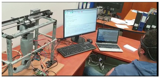
Figure 1.
A prosthesis operated by means of a neural headset: neurally actuated prosthetic prosthesis (NAPP).
The prosthesis consists of a knee actuated via a servomotor, and an ankle also actuated via a servomotor. The solution, to be developed in the future, is intended to be used as a prosthesis for people whose lower limb (from the knee down) has been amputated, or to equip a medium-sized humanoid robot. To set the prosthesis in motion, a system/frame was made that also had a stepper motor for longitudinal movement. An actuation was also performed on the two servomotors, with the help of a neural headset. The primary intention was to create a prosthetic prosthesis that could be operated with the help of brain waves.
The main contributions of the paper consist of:
- The creation of a prosthesis of the lower part of the leg, an experimental model operated with electric motors (brushless);
- creating a command and control system that allows the foot to be operated with the help of a neural headset;
- creating the framework concept for the design of a foot prosthesis so that, in the later stage of development, we can create a prosthesis that respects the real configuration of the foot, and is capable of responding to real mechanical demands;
- creating the analytical model that describes the kinematic and dynamic operation of such a prosthesis;
- the creation of the numerical model, which allows us to highlight the dynamic demands of the prosthesis;
- obtaining the areas where tension concentrators appear, something that will be solved via a new configuration/structure for the future prosthesis;
- highlighting the limitations of the experimental model created.
The training framework for the prosthetic system (bionic leg) was made in the Laboratory of the Materials Resistance Department of the POLITEHNICA University in Bucharest, in collaboration with the Center of Excellence in Robotics and Autonomous Systems (CERAS). The developed solution is an experimental model, validated in the research laboratory. Although the analyzed system is a consumer of electricity, in the future, a compartment for Li-ion batteries will be made in the calf, with the possibility of having a portable battery on the operator.
The paper is structured as follows: Section 2 discusses how the instrumentation was used to test the operation of the bionic foot assembly, in order to determine the correlation between longitudinal axis displacement and vibrations in the foot and ankle area. Also presents the results obtained analytically regarding the kinematics and dynamics of the foot. Section 3 presents the results: experimental measurements, mechanical test results of the test pieces and the numerical analysis, and describes the comparative analysis of the results obtained experimentally, and those obtained from the numerical analysis. Section 4 presents the conclusions, and the potential options for further development.
2. Materials and Methods
The experimental tests carried out during this research consisted of the determination of the material characteristics, the displacement along the longitudinal axis, and the vibrations at two points on the foot. The experimental setup for testing the bionic leg is shown in Figure 2.
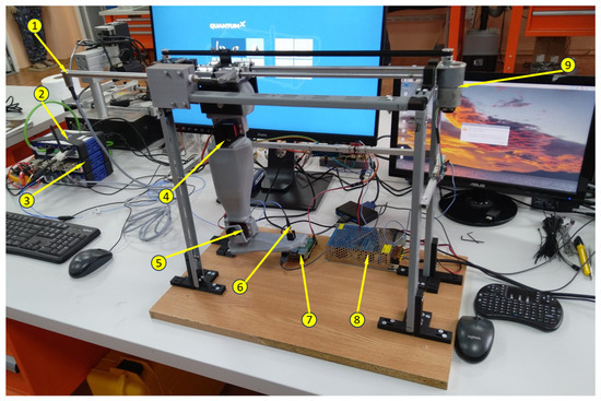
Figure 2.
The bionic leg experimental setup: 1. HBM’s WA200-series displacement sensor #260510079; 2. QuantumX CX22B-W computer S/N F0F9578297C8; 3. strain gauge MX840B S/N 0009E520A43; 4. Servomotor K-Power HBL090 ball joint; 5. K-Power HBL090 ankle actuator; 6. Accelerometer PCB Piezotronics 356A43 S/N LW348378; 7. Raspberry Pi4 model B 4GB RAM; and 8. power supply; 9. Motor JGB37-520 (12 V, 1:90, 107 RPM).
2.1. Materials Used
The component elements of the leg were fabricated using the method of 3D printing from PLA (polylactic acid or polylactide) [30]. PLA is a bioabsorbable biopolymer produced from non-toxic renewable raw material [31]. The solution chosen regarding the material from which the leg is made, at this point in the research, also took into account the fact that PLA is considered good for medical applications [32]. We make this statement because, at a later stage of development, the bionic leg will come into contact with the human body. The physical properties of PLA, according to [33], are shown in Table 1.

Table 1.
Physical and mechanical properties of PLA 1 [33].
The PLA used is soluble in chloroform, methylene chloride, etc., and degrades via hydrolysis after exposure to a moist environment.
To validate the physical–mechanical properties, three types of samples were made, to test the material under compression, stretching, and bending stresses (Figure 3). The material characteristics can be found in Table 2.
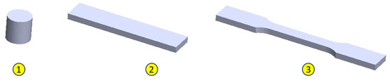
Figure 3.
Specimens for determining the physical/mechanical characteristics of the PLA used in the construction of the bionic leg: 1. compression test specimen; 2. tensile test specimen; 3. test specimen for bending stress.
Table 2.
The printing characteristics of the leg specimens and components are as follows.
After 10 samples were printed for each type of test, they were measured, and the dimensions in Table 3, Table 4 and Table 5 were obtained.
Table 3.
The specimen dimensions required for compression.
Table 4.
The specimen dimensions required for traction.
Table 5.
The specimen dimensions required for bending.
2.2. The Technology for Making the Leg
The component elements of the bionic prosthesis after the design phase were processed in a specific language for the PRUSA i3 MK3 3D printer (Figure 4 and Figure 5).
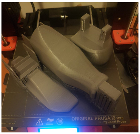
Figure 4.
The 3D printing of the three component elements of the bionic leg.
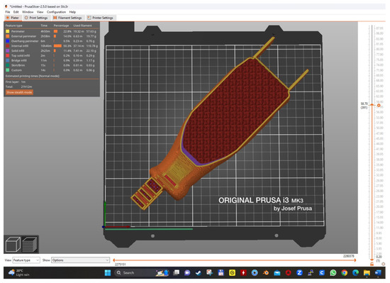
Figure 5.
An example of the 3D printing of the calf, with characteristics according to Table 2.
As already stated, the purpose of the research is to determine the resistance capacity of a prototype foot made using additive technology (3D printing from PLA) to withstand the dynamic demands produced by its movement, according to an imposed law. The component parts of the foot are the sole (Figure 6a), the lower leg (Figure 6b), and the knee (Figure 6c).
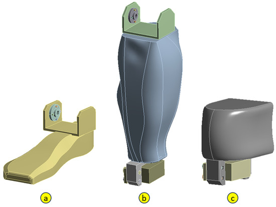
Figure 6.
The component elements of the bionic foot: a. sole; b. calf; c. knee.
From a constructive/assembly point of view, we have the following:
- Sole:
- The foot (monobloc piece made from PLA);
- The motor attachment bushing, positioned next to the ankle (aluminum);
- Fixing screws between the bushing and the foot (steel);
- Calf:
- The gamba (monobloc part made of PLA);
- The sole drive actuator (considered aluminum);
- Actuator mounting bolts (steel);
- The motor mounting bush, positioned next to the knee (aluminum);
- Clamping screws between the bushing and the shank (steel);
- Knee:
- The knee (monobloc piece from PLA);
- The calf actuator (considered aluminum);
- Actuator mounting bolts (steel).
The inside of the calf and foot were printed with 30% infill, and the outer walls were printed with 1 mm thickness. Due to this aspect, the two components were geometrically modeled separately. Figure 7 shows the outside of the calf (transparent) printed with 100% fill, and the inside (opaque) printed with 30% fill.
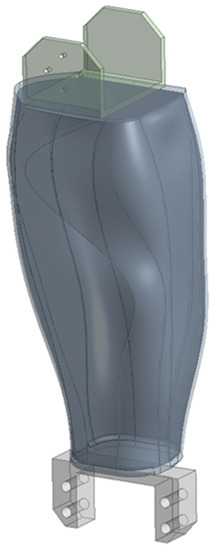
Figure 7.
The calf geometry, with a separately molded interior.
The movement of the experimental model is to be controlled with the help of an interface (neural helmet) that reads and interprets brain impulses. As the interface is in the design and testing phase, in this phase, there is no problem with stepping on an obstacle, so the forces that apply to the experimental model are weight and inertial forces.
2.3. Methods
2.3.1. Kinematics
To estimate the forces in the leg joints, linear motion laws for the rotation angle of the output shaft were imposed on the actuators. Thus, in an interval of 5 s, the shaft of each servomotor rotates by an angle of 20 degrees. The resulting kinematics are simple if a schematization is adopted, as in Figure 8 and Figure 9. According to this schematization, the velocities and accelerations of the prosthesis components are determined.
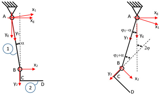
Figure 8.
Schematic of the foot in the initial position, and at one point in time, t.
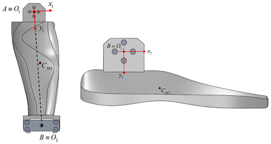
Figure 9.
The position of the local coordinate systems.
The calf is marked with 1, the sole with 2, the joint between the knee and calf with A, and the joint between the calf and sole with B. The global system is denoted , and the local systems related to the calf and sole are denoted and (Table 6). Between the line of the calf joints, for the considered vertical position, there is an angle of .
Table 6.
The calf and sole mass characteristics.
The position vector of the joint in B is given by the following vector relation:
where is the angle between the vertical and segment AB, measured clockwise; is the length of segment AB.
The law of variation of angle is , being the same as , and and are the vertices of the global coordinate system.
Via derivation with respect to time, the velocity results and the second-order derivative give the expression of the acceleration. As the derivative of the angle is the angular velocity, it is noted that it is constant over time: . For simplification, we write ; consequently, .
The vector expressions for velocity and acceleration are as follows:
For the center of mass of the calf, the position relative to the local system is given by
Using the relationship between the mobile and the fixed system’s calf-related feeders,
which results in the position vector with respect to the fixed system:
The acceleration of the center of mass is obtained via differentiating twice with respect to time:
For the center of mass of the sole, we determine the position vector from the following relationship:
The coordinate system related to the sole, with the pourers and , is rotated relative to the fixed coordinate system by the angle . The connection between the mobile and the fixed systems is given by the following relations:
Substituting vertices into the position vector relation of the center of mass , we obtain:
By deriving the speed results with respect to time, and by deriving twice, the acceleration is obtained. The vector expressions with respect to the global system are:
Figure 10 and Table 7 show the coordinate systems used for the sole. The system is the system bound to the sole, and the coordinate systems and are the coordinate systems of the sole-bound accelerometers, which have their origins at the acceleration measurement points.
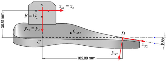
Figure 10.
The coordinates of the positions where the accelerometers were attached.
Table 7.
The accelerometer positions relative to the sole-bound system.
Accelerometer measurement directions:
- In position 1, they are overlapped with the axes of the coordinate system linked to the sole;
- In position 2, the measurement directions are rotated by 9.88° trigonometrically.
Substituting the moving vertices of the coordinate system related to the base into the acceleration relation of point B results in the following expression:
This expression could also be found through directly writing the acceleration with respect to the system connected to the sole, knowing the direction (AB) and the module .
This expression is necessary for the interpretation of the experimental results, as it is also valid for the coordinate system of sensor 1.
For point D, which is the second position of the accelerometer, the relationships are similar to those of the center of mass. The position vector, velocity, and acceleration relative to the fixed system are given by:
With respect to the local system of the sole, using relations (10) and (11), it follows that:
and the expression for the acceleration of point D relative to the system attached to the sole is:
This relationship can also be obtained from Euler’s formula written for the sole:
where has the direction BD, with the orientation from D to B and the module , and , because .
Compared to the sensor-related system , which is rotated relative to the system with the angle , the acceleration becomes
In order to highlight the movement described by the above laws, three-way accelerometers (PCB Piezotronics 356A43 S/N LW348378) were used. Accelerometers were attached to the foot in two positions: on the sole, and on the axis of the calf–foot joint.
2.3.2. Dynamics
To determine the forces in the joints, we isolate the system (Figure 11). For each body, we write the momentum theorem with respect to the fixed reference system, and the kinetic momentum theorem with respect to the center of mass.
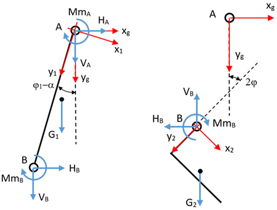
Figure 11.
The calf and sole insulation.
For the calf (body 1), we obtain the following relations:
where is the mass of the calf, is the weight of the calf, and are the components of the acceleration of the center of mass (relation (8)), and and are the motor moments in the joints, which produce the movement.
The moment about the center of mass of the force is determined via
with the component along the Oz axis being
Similarly, the components of the other moments result in the following:
For the calf (body 2), we obtain the following relations:
where is the mass of the calf, is the weight of the calf, and and are the components of the acceleration of the center of mass (relation (14)).
From relations (32) and (33), we obtain the force components in joint B, , and :
and from relation (34), the motor moment in joint B is given by
From relations (24)–(26), we obtain the components of the connecting force in joint A, and the motor moment from this joint:
2.3.3. Equipment Used in the Determination of Mechanical Characteristics
In order to determine the mechanical characteristics, two pieces of equipment were used; namely, the INSTRON 8872 universal testing machine (Figure 12), and the Dantec image correlation system (Figure 13). All the mechanical tests were performed at 1 mm/min.
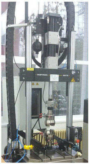
Figure 12.
INSTRON 8872 universal testing machine [30].
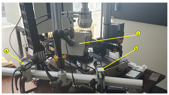
Figure 13.
Image correlation system (a—Camera 1, b—Camera 2, c—light source).
The characteristics of the INSTRON 8872 are shown in Table 8.
Table 8.
Specimen dimensions required for bending.
The specifications of the image correlation system are shown in Table 9.
Table 9.
Specimen dimensions required for bending.
Figure 14 shows the tested samples.
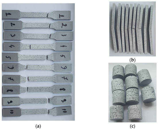
Figure 14.
Tested specimens: (a) traction, (b) bending, (c) compression.
The specific deformations were taken from the application of the image correlation method, and the values of the normal stresses appearing during the tensile and compressive stresses were determined via the following relationship:
where F is the axial force applied to the specimen; and A is the cross-sectional area of the specimen.
For the three-point bending test, the formulas used to calculate the normal stress and the specific strain were as follows:
where s is the distance between the supports (support span); d is the sample arrow; b is the width of the sample; and h is the thickness of the specimen.
2.3.4. Simulation via the Finite Element Method
ANSYS software was used for finite element modeling. The modeling was performed for a transient regime, using the Transient Structural module.
The contacts used between these components are as follows:
- For the sole:
- o
- A “frictionless” type for the contact between the foot and the clamping bush with the servomotor;
- o
- A “bound” type for the rest of the contacts;
- For the calf:
- o
- A “frictionless” type for the contact between the calf and the clamping bush with the servomotor in the knee, and for the contact between the foot actuation servomotor and the calf;
- o
- A “bound” type for the rest of the contacts;
- For the knee:
- o
- A “frictionless” type for the contact between the knee and the calf actuation servomotor;
- o
- A “bound” type for the rest of the contacts.
Between the sole and the calf, and between the calf and the knee, respectively, “revolute” connections were defined between the shafts of the actuators and the connecting bushings. This type of link allows the imposition of boundary conditions on angular displacements, angular velocities, or angular accelerations.
The finite element discretization, and a detail of the discretization in the knee area, are shown in Figure 15. An average element size of 12 mm was used for the discretization, with refinement on contact surfaces with an average size of 1 mm, resulting in 120,592 nodes and 69,622 elements.
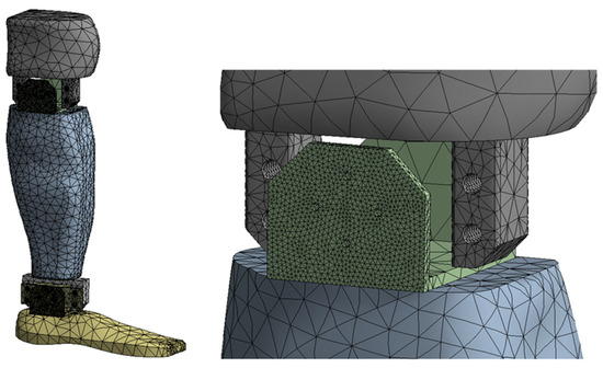
Figure 15.
Finite element discretization.
Zero displacements were considered on the upper surface of the knee. In the “revolute”-type links, angular displacements were imposed, according to the law presented in Figure 16.
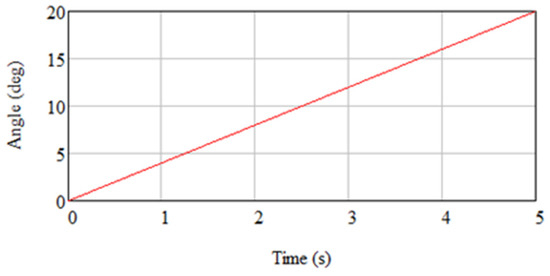
Figure 16.
“Revolved” connections with the imposition of angular displacements.
The mass forces due to the user’s weight were also taken into account, defining the gravitational acceleration (Figure 17).
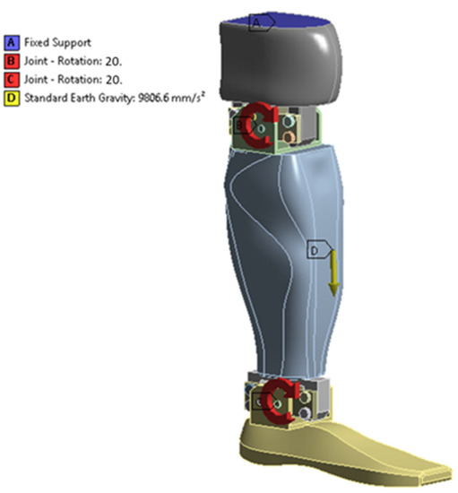
Figure 17.
The boundary conditions, gravitational acceleration, and rotations imposed in the joints on the geometric configuration from the initial time instant.
The analysis was transient, with a time interval of seconds, and a minimum time step of . The displacements were considered large, and the results were saved at each time step.
3. Results
3.1. Experimental Measurements
To allow the realization of the movements of the leg prosthesis, it was equipped with hardware, as follows: Raspberry Pi 4, two servo motors, a motor driver module, and an external power supply (this variant being sufficient to demonstrate the concept of the neural control of the prosthesis) and, for controlling the prosthesis with the power of the mind, an EMOTIV Insight headset (Figure 1) was used (this being responsible for capturing electrical signals from the brain, and converting them into specific commands, which could later be used to control the bionic lower limb prosthesis). The testing of the implemented system was carried out with a healthy male participant, who used the neural helmet to train two commands necessary for the movement of the leg prosthesis. Compared to other advanced headsets that contain many electrodes, the performance of the system is relatively good in terms of the EEG signal obtained from the EMOTIV Insight Neuronal Headset, because it provides the desired decoding and processing for the brain signals.
Figure 18 and Figure 19 show the experimentally determined acceleration components, with an acquisition frequency of 300 Hz, for the two accelerometers. Analytically determined acceleration variations are also presented on the same graphs.
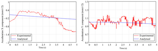
Figure 18.
The time variation in the experimentally and analytically determined acceleration components for sensor 1.
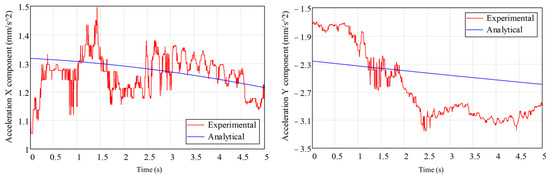
Figure 19.
The time variation in experimentally and analytically determined acceleration components for sensor 2.
3.2. Mechanical Test Results
Figure 20, Figure 21 and Figure 22 show the characteristic curves for all ten specimens subjected to tension, compression, and bending, respectively.
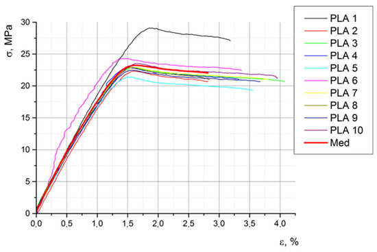
Figure 20.
The stress–strain curves of the ten specimens subjected to traction.

Figure 21.
The stress–strain curves of the ten specimens subjected to compression.
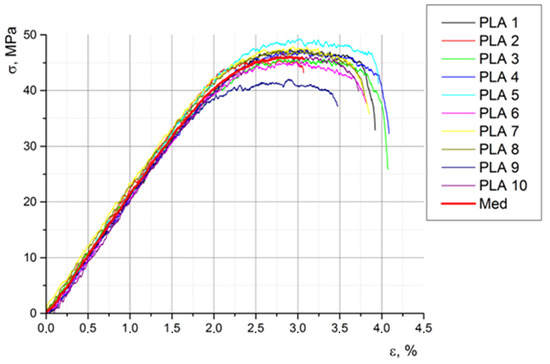
Figure 22.
The stress–strain curves of the ten specimens subjected to bending.
Table 10 shows the main mechanical properties obtained via the tensile test.
Table 10.
The mechanical characteristics of the tensile specimens.
Following the compression test, a series of mechanical characteristics of PLA were obtained, which are presented in Table 11.
Table 11.
The mechanical characteristics of the samples subjected to compression.
As a result of the bending tests, the following mechanical properties of PLA were obtained, as shown in Table 12.
Table 12.
The mechanical characteristics of the samples subjected to compression.
Following the statistical analysis of the experimental results, we concluded that the average values, regarding the mechanical characteristics of the material from which the prosthesis was made (experimental model), were sufficient for the present study. In further development, we will perform a statistical analysis regarding the behavior of the bionic prosthesis in response to the different (real) demands that will be identified as reasonable in the simulation of bipedal walking.
3.3. The Results Obtained from the Analysis via the Finite Element Method
Figure 23, Figure 24, Figure 25, Figure 26, Figure 27 and Figure 28 show the resulting displacements in the components made of PLA, for the times of 0.833, 1.667, 2.5, 3.333, 4.167, and 5 s.
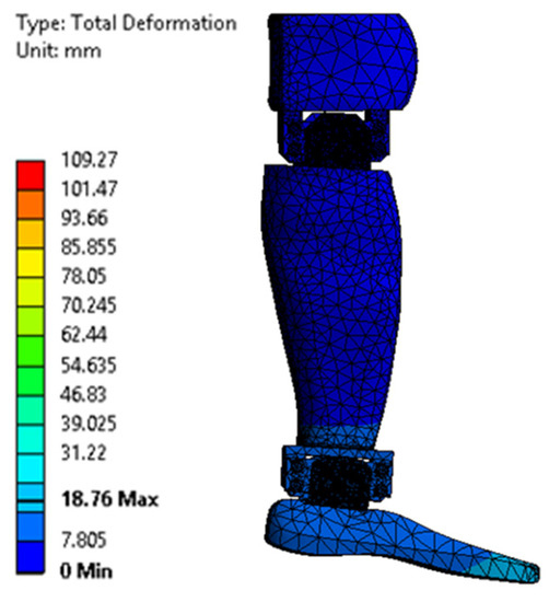
Figure 23.
Total displacement at 0.833 s.
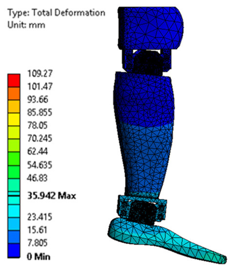
Figure 24.
Total displacement at 1.667 s.
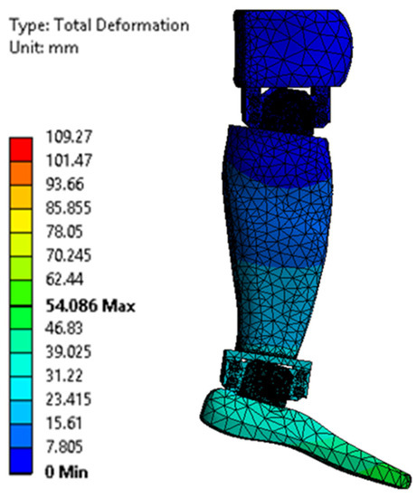
Figure 25.
Total displacement at 2.5 s.
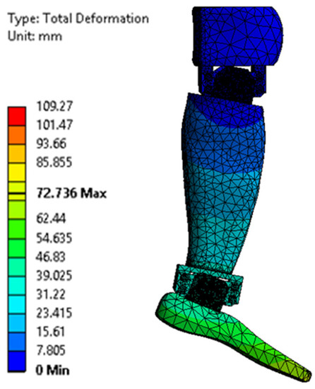
Figure 26.
Total displacement at 3.333 s.
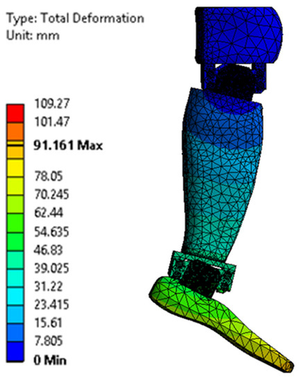
Figure 27.
Total displacement at 4.167 s.
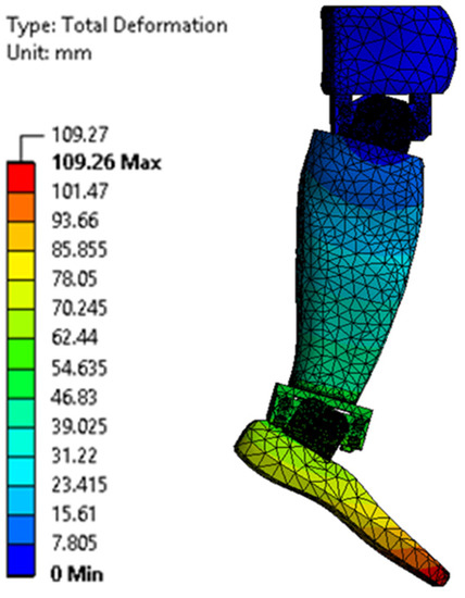
Figure 28.
Total displacement at 5 s.
Figure 29, Figure 30, Figure 31, Figure 32, Figure 33 and Figure 34 show the equivalent stresses in the components made of PLA, for the times of 0.833, 1.667, 2.5, 3.333, 4.167, and 5 s.
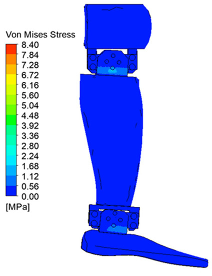
Figure 29.
Von Mises stress at 0.833 s.
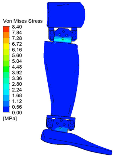
Figure 30.
Von Mises stress at 1.667 s.
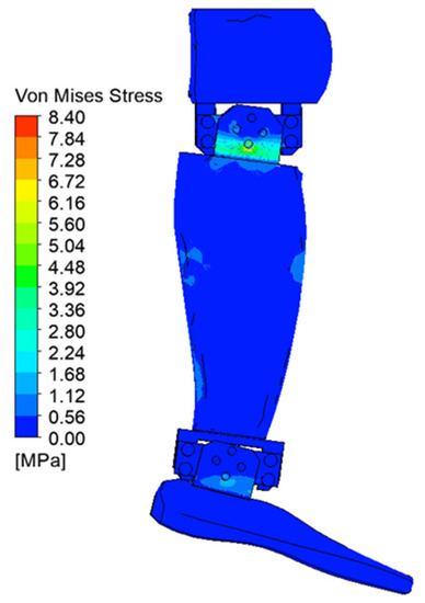
Figure 31.
Von Mises stress at 2.5 s.
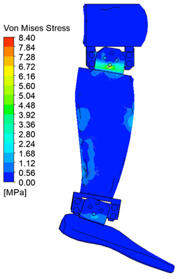
Figure 32.
Von Mises stress at 3.333 s.
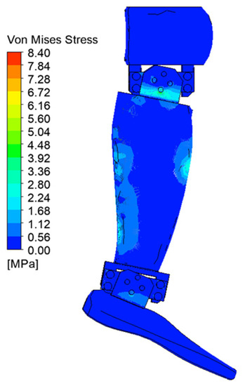
Figure 33.
Von Mises stress at 4.167 s.
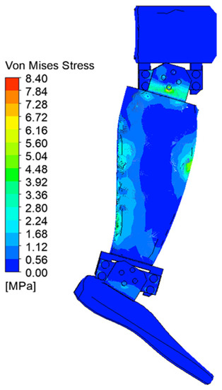
Figure 34.
Von Mises stress at 5 s.
The maximum equivalent von Mises stress is reached when the angle of inclination of the calf to the vertical is maximum, i.e., 20°. This value is reached on the inside of the calf clamping yoke, in the area of contact with the servomotor clamping bush, in the knee joint. Figure 35 shows a detail of the maximum stress area. The ultimate stress is lower than the breaking strength of the PLA material.
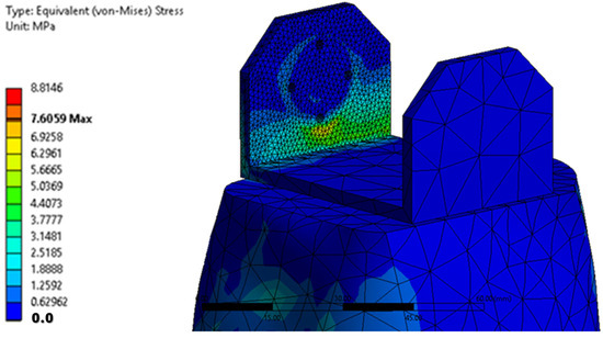
Figure 35.
A detail of the maximum equivalent voltage area.
In the knee joint, the time variations in force and moment by components, expressed with respect to the local system, are presented in Figure 36, Figure 37, Figure 38 and Figure 39. The maximum stress is observed when the leg and sole are rotated by 20 degrees, with the moment in the joint reaching the maximum value of 717.05 N mm.
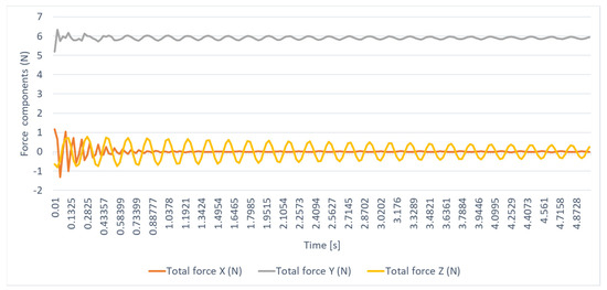
Figure 36.
The time variation in the knee–joint bond force components.
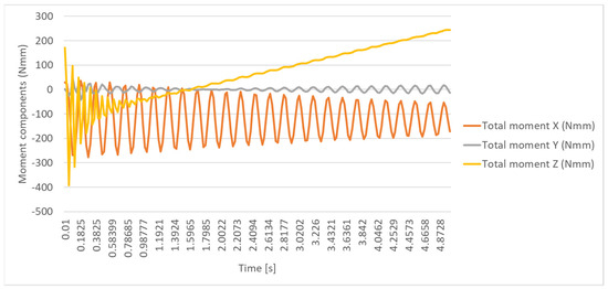
Figure 37.
The time variation in the link moment components in the knee joint.
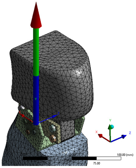
Figure 38.
The resultant force.
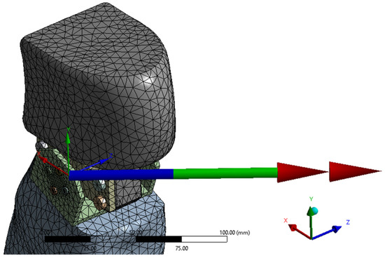
Figure 39.
The resulting moment.
For a more accurate calculation in the zone of maximum stresses, a simplified geometry was used (Figure 40, with the coordinate system of the knee joint), via the sectioning of the calf with a plane at a distance of 20 mm from the knee yoke.
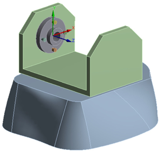
Figure 40.
The simplified geometry of the knee joint.
The geometry was finely discretized in the contact area between the actuator bushing and the knee yoke, with 221,160 nodes and 135,931 elements (Figure 41).
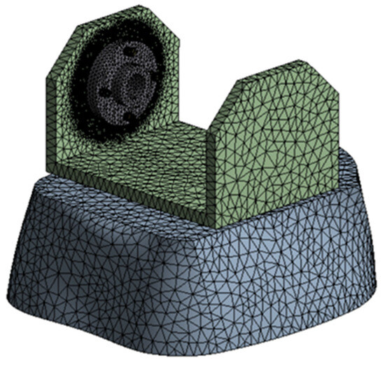
Figure 41.
The discretization of the knee joint in the contact area between the actuator bushing and the knee joint.
“Frictionless” contacts were defined between the clamping screws and the knee yoke, and between the servomotor clamping bushing and the knee yoke, and “bound” contacts were defined between the screws and the clamping bushing. In the lower part of the structure, on the section plane, the nodes were considered blocked. The maximum force and moment determined in the transient analysis were imposed on the inner cylindrical surface of the clamping bush.
Figure 42 shows the von Mises equivalent stresses for the PLA component. A maximum stress of 12.84 MPa is noted in the vicinity of the screw hole at the bottom of the knee yoke. Below this area is the value of the voltage determined during the transient calculation.
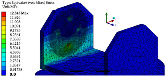
Figure 42.
The equivalent von Mises stresses in PLA.
Figure 43 and Figure 44 show the equivalent stresses in the servomotor mounting bushing, and the knee yoke mounting bolts, respectively. It is noted that the maximum stress is small compared to the yield stress of the two materials.
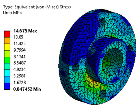
Figure 43.
The von Mises equivalent stresses from the bushing with the servomotor.
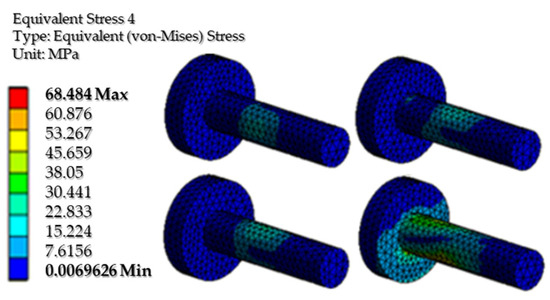
Figure 44.
The von Mises equivalent stresses from the fastening screws.
4. Discussion
It is noted both from the experimental results, and from the finite element model, that vibrations exist in the mechanical system when it is in motion. This aspect is due to the fact that, at the initial moment, the leg is in static equilibrium, and when the actuators act, the components must accelerate from zero rotational speed to the imposed speed of 0.069 rad/s. This action produces vibration in the absence of torque control. Another solution is to use a function for the displacement law that ensures acceleration and deceleration over a longer period of time, with an intermediate interval of constant speed. As vibrations cannot be eliminated, a future research direction would be to study the fatigue of PLA components.
From the analysis of Figure 18 and Figure 19, in which the components of the accelerations on the measurement directions of the accelerometers have been determined experimentally and analytically, a good agreement is noted. For better control of the position of the leg components, and to more easily compare experimental data with analytical or numerical data, it is necessary to use angular displacement sensors (encoders).
Another future direction of interest is the obstacle approach. In this case, the forces that apply to the leg structure can increase substantially. For this reason, we will introduce an elastic joint system.
Regarding the elastic and mechanical characteristics of PLA, Figure 45 shows the values of the transverse contraction coefficient for the tensile and compression tests. The transverse shrinkage coefficient could not be obtained following the three-point bending test.
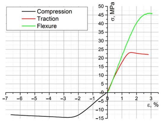
Figure 45.
The characteristic curves of the three tests performed for PLA.
Figure 46 shows the values of the longitudinal modulus of elasticity, determined as a result of the three tests performed.
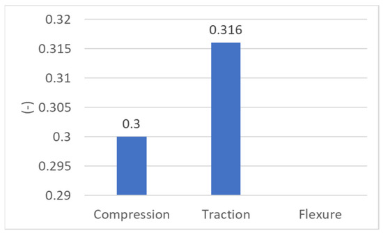
Figure 46.
The values of the transverse shrinkage coefficient of the studied PLA.
The yield strength and fracture strength values, obtained via the mechanical tests performed, are presented in Figure 47, Figure 48 and Figure 49.
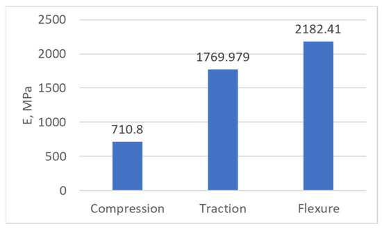
Figure 47.
The values of the longitudinal modulus of elasticity of the PLA.
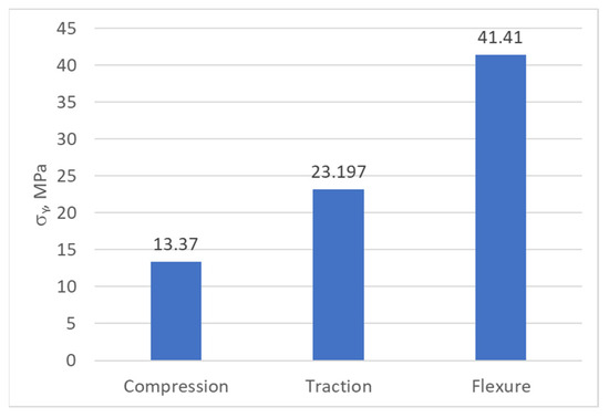
Figure 48.
The yield strength values of the PLA.
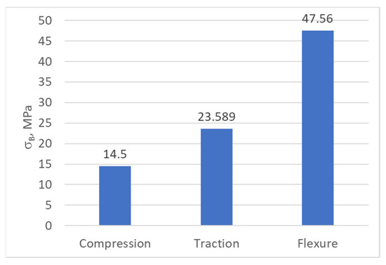
Figure 49.
The breaking point values of the PLA.
One conclusion of the mechanical results is that, due to the way the prosthesis is printed (the degree of filling), following the tests performed, the behavior of the material is different depending on the type of request. Through analyzing the obtained results, it can be concluded that the prosthesis withstands static and dynamic conditions without any problem.
Another conclusion would be that, instead of single-axis servomotors, we should use dual-axis servomotors, which would allow a cylindrical joint on both sides of the yoke. This will lead to an increased stiffness in the assembly. We will also further analyze the possibility of creating a coaxial passive joint with the servomotor axis on the opposite side of the yoke. These constructive variants will increase the rigidity of the system, reducing the level of vibrations.
For a better replication of the lower limb, we will try to re-smooth the fingers of the prosthesis (especially for the joint area near the toes), using the topology optimization method [29]. We will use attached springs, so that we can mimic their elasticity or stiffness, which is necessary in order to be able to simulate bipedal walking.
To determine the effort in the prosthesis that we will make (based on the model described), we will use a force sensor based on metal ionic composites (IP-MCs) [34], which are smart transducers made of materials that bend in response to low-voltage stimuli, and generate voltage in response to bending.
Author Contributions
Conceptualization, M.-V.D., A.H. and N.G.; methodology, F.B. and D.G.; software, N.G., C.M., I.O. and D.G.; validation, A.Ș., L.Ș.G. and F.B.; formal analysis, M.-V.D. and A.Ș.; investigation, M.-V.D., A.H., F.B., N.G. and A.Ș.; resources, M.-V.D. and I.O.; data curation, I.O.; writing—original draft preparation, M.-V.D.; writing—review and editing, A.H., N.G. and C.M.; visualization, N.G. and C.M.; supervision, A.H. and N.G.; project administration, I.O. All authors have read and agreed to the published version of the manuscript.
Funding
This research received no external funding.
Institutional Review Board Statement
Not applicable for studies not involving humans or animals.
Informed Consent Statement
Not applicable.
Data Availability Statement
Not applicable.
Conflicts of Interest
The authors declare no conflict of interest.
References
- World Health Organization. Standards for Prosthetics and Orthotics Part 1: Standards; World Health Organization: Geneva, Switzerland, 2017; ISBN 9789241512480. Available online: https://apps.who.int/iris/bitstream/handle/10665/259209/9789241512480-part1-eng.pdf?sequence=1&isAllowed=y (accessed on 7 June 2023).
- Ziegler-Graham, K.; MacKenzie, E.J.; Ephraim, P.L.; Travison, T.G.; Brookmeyer, R. Estimating the prevalence of limb loss in the United States: 2005 to 2050. Arch. Phys. Med. Rehabil. 2008, 89, 422–429. [Google Scholar] [CrossRef] [PubMed]
- Wired. The Future of Prosthetics Could Be This Brain-Controlled Bionic Leg. 2013. Available online: https://www.wired.com/2013/10/is-this-brain-controlled-bionic-leg-the-future-of-prosthetics/ (accessed on 7 June 2023).
- Bellman, R.D.; Holgate, M.A.; Sugar, T.G. SPARKy 3: Design of an Active Robotic Ankle Prosthesis with Two Actuated Degrees of Freedom Using Regenerative Kinetics. In Proceedings of the 2008 2nd IEEE RAS & EMBS International Conference on Biomedical Robotics and Biomechatronics, Scottsdale, AZ, USA, 19–22 October 2008; pp. 511–516. [Google Scholar] [CrossRef]
- Hitt, J.; Holgate, M.; Bellman, R.; Sugar, T.; Hollander, K. The SPARKy (Spring Ankle with Regenerative Kinetics) Project: Design and Analysis of a Robotic Transtibial Prosthesis. In Proceedings of the ASME International Design Engineering Technical Conference and Computers and Information in Engineering Conference, Las Vegas, NV, USA, 4–7 September 2007. [Google Scholar] [CrossRef]
- U.S. Army Medical Research and Development Command (USAMRDC). Available online: https://mrdc.health.mil/ (accessed on 7 June 2023).
- Flynn, L.; Geeroms, J.; Jimenez-Fabian, R.; Heins, S.; Vanderborght, B.; Munih, M.; Molino Lova, R.; Vitiello, N.; Lefeber, D. The Challenges and Achievements of Experimental Implementation of an Active Transfemoral Prosthesis Based on Biological Quasi-Stiffness: The CYBERLEGs Beta-Prosthesis. Front. Neurorobot. 2018, 12, 80. [Google Scholar] [CrossRef]
- New Atlas. Available online: https://newatlas.com/amp-foot-20-prosthesis-mimics-human-ankles-spring/24801/ (accessed on 7 June 2023).
- Staros, A. The sach (solid-ankle cushion-heel) foot. Orthop. Prosthet. Appl. J. 1957, 11, 23–31. [Google Scholar]
- Hafner, B.J.; Sanders, J.E.; Czerniecki, J.M.; Fergason, J. Transtibial energy-storage-and-return prosthetic devices: A review of energy concepts and a proposed nomenclature. Bull. Prosthet. Res. 2002, 39, 1–11. [Google Scholar]
- Mauch, H. Stance control for above-knee artificial legs-design considerations in the s-n-s knee. Bull. Prosthet. Res. 1968, 20, 61–72. [Google Scholar]
- Au, S.; Herr, H. Powered ankle-foot prosthesis: The importance of series and parallel motor elasticity. IEEE Robot. Autom. Mag. 2008, 15, 52–59. [Google Scholar] [CrossRef]
- Petrone, N.; Costa, G.; Foscan, G.; Gri, A.; Mazzanti, L.; Migliore, G.; Cutti, A.G. Development of Instrumented Running Prosthetic Feet for the Collection of Track Loads on Elite Athletes. Sensors 2020, 20, 5758. [Google Scholar] [CrossRef]
- Lawson, B.E.; Mitchell, J.; Truex, D.; Shultz, A.; Ledoux, E.; Goldfarb, M. A robotic leg prosthesis: Design, control, and implementation. IEEE Robot. Autom. Mag. 2014, 21, 70–81. [Google Scholar] [CrossRef]
- Rouse, E.J.; Mooney, L.M.; Herr, H.M. Clutchable series-elastic actuator: Implications for prosthetic knee design. Int. J. Rob. Res. 2014, 33, 1611–1625. [Google Scholar] [CrossRef]
- Pfeifer, S.; Pagel, A.; Riener, R.; Vallery, H. Actuator with angle dependent elasticity for biomimetic transfemoral prostheses. IEEE/ASME Trans. Mechatron. 2014, 20, 1384–1394. [Google Scholar] [CrossRef]
- Grabowski, A.M.; D’Andrea, S. Effects of a powered ankle-foot prosthesis on kinetic loading of the unaffected leg during level-ground walking. J. Neuroeng. Rehabil. 2013, 10, 49. [Google Scholar] [CrossRef] [PubMed]
- Cherelle, P.; Mathijssen, G.; Wang, Q.; Vanderborght, B.; Lefeber, D. Advances in Propulsive Bionic Feet and Their Actuation Principles. Adv. Mech. Eng. 2014, 6, 984046. [Google Scholar] [CrossRef]
- Huang, Q.; Li, B.; Xu, H. The Design and Testing of a PEA Powered Ankle Prosthesis Driven by EHA. Biomimetics 2022, 7, 234. [Google Scholar] [CrossRef] [PubMed]
- Di Gregorio, R.; Vocenas, L. Identification of Gait-Cycle Phases for Prosthesis Control. Biomimetics 2021, 6, 22. [Google Scholar] [CrossRef] [PubMed]
- Hayot, C. Analyse Biomécanique 3D de la Marche Humaine: Comparaison des Modèles Mécaniques. Ph.D. Thesis, University of Poitiers, Poitiers, France, 2010. Available online: https://www.theses.fr/2010POIT2342 (accessed on 7 June 2023).
- Hatze, H. A mathematical model for the computational determination of parameter values of anthropomorphic segments. J. Biomech. 1980, 13, 833–843. [Google Scholar] [CrossRef]
- Grimmer, M.; Holgate, M.; Holgate, R.; Boehler, A.; Ward, J.; Hollander, K.; Sugar, T.; Seyfarth, A. A powered prosthetic ankle joint for walking and running. BioMedical Eng. OnLine 2016, 15 (Suppl. 3), 141. [Google Scholar] [CrossRef]
- Bilal, M.; Rizwan, M.; Maqbool, H.F.; Ahsan, M.; Raza, A. Design optimization of powered ankle prosthesis to reduce peak power requirement. Sci. Prog. 2022, 105, 368504221117895. [Google Scholar] [CrossRef]
- Frank, S.; Huseyin Atakan, V.; Jason, M.; Withrow, T.; Goldfarb, M. Design and control of an active, electrical, knee and ankle prosthesis. In Proceedings of the 2008 2nd IEEE RAS & EMBS International Conference on Biomedical Robotics and Biomechatronics, Scottsdale, AZ, USA, 19–22 October 2008; pp. 523–528. [Google Scholar] [CrossRef]
- Song, K.-Y.; Behzadfar, M.; Zhang, W.-J. A Dynamic Pole MotionApproach for Control of Nonlinear Hybrid Soft Legs: A preliminary Study. Machines 2022, 10, 875. [Google Scholar] [CrossRef]
- Liu, S.O.; Zhang, H.B.; Yin, R.X.; Chen, A.; Zhang, W.J. Flexure Hinge Based Fully Compliant Prosthetic Finger. In Lecture Notes in Networks and Systems, Proceedings of the SAI Intelligent Conference (IntelliSys) 2016, London, UK, 21–22 September 2016; Springer: Cham, Switzerland, 2016; pp. 839–849. [Google Scholar] [CrossRef]
- Sun, Y.; Lueth, T.C. Design of Bionic Prosthetic Fingers Using 3D Topology Optimization. In Proceedings of the 43rd Annual International Conference of the IEEE Engineering in Medicine & Biology Society (EMBC), Guadalajara, Mexico, 1–5 November 2021; pp. 4505–4508. [Google Scholar] [CrossRef]
- Zheng, Y.; Cao, L.; Qian, Z.; Chen, A.; Zhang, W. Topology optimization of a fully compliant prosthetic finger: Design and testing. In Proceedings of the 6th IEEE International Conference on Biomedical Robotics and Biomechatronics (BioROb), Singapore, 26–29 June 2016; pp. 1029–1034. [Google Scholar] [CrossRef]
- Savioli Lopes, J.M.; Jardini, A.L.; Maciel Filho, R. Poly (Lactic Acid) Production for Tissue Engineeering Applications. Procedia Eng. 2012, 42, 1402–1413. [Google Scholar] [CrossRef]
- Lasprilla, A.J.R.; Martinez, G.A.R.; Lunelli, B.H.; Jardini, A.L.; Filho, R.M. Poly-lactic acid synthesis for application in biomedical devices—A review. Biotechnol. Adv. 2012, 30, 321–328. [Google Scholar] [CrossRef]
- Rasal, R.M.; Janorkar, A.V.; Hirta, D.E. Poly (Lactic Acid) Modifications. Prog. Polym. Sci. 2010, 30, 338–356. [Google Scholar] [CrossRef]
- Farah, S.; Anderson, D.G.; Langer, R. Physical and mechanical properties of PLA, and their functions in widespread applications—A comprehensive review. Adv. Drug Deliv. Rev. 2016, 107, 367–392. [Google Scholar] [CrossRef] [PubMed]
- Bonomo, C.; Fortuna, L.; Giannone, P.; Graziani, S.; Strazzeri, S. A resonant force sensor based on ionic polymer metal composites. Smart Mater. Struct. 2007, 17, 015014. [Google Scholar] [CrossRef]
Disclaimer/Publisher’s Note: The statements, opinions and data contained in all publications are solely those of the individual author(s) and contributor(s) and not of MDPI and/or the editor(s). MDPI and/or the editor(s) disclaim responsibility for any injury to people or property resulting from any ideas, methods, instructions or products referred to in the content. |
© 2023 by the authors. Licensee MDPI, Basel, Switzerland. This article is an open access article distributed under the terms and conditions of the Creative Commons Attribution (CC BY) license (https://creativecommons.org/licenses/by/4.0/).