
Neuro-Inspired Signal Processing in Ferromagnetic Nanofibers


Abstract
1. Introduction
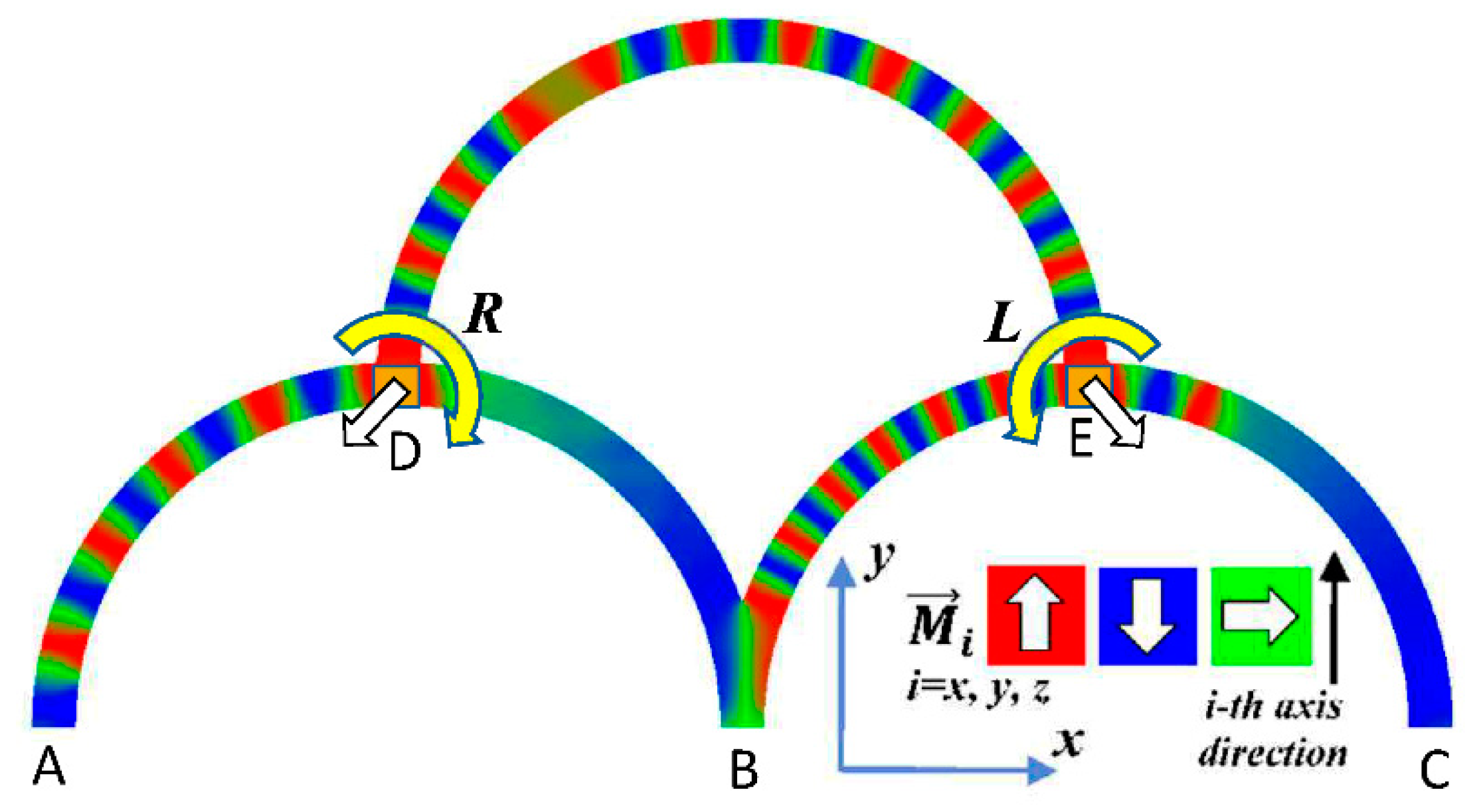
2. Materials and Methods
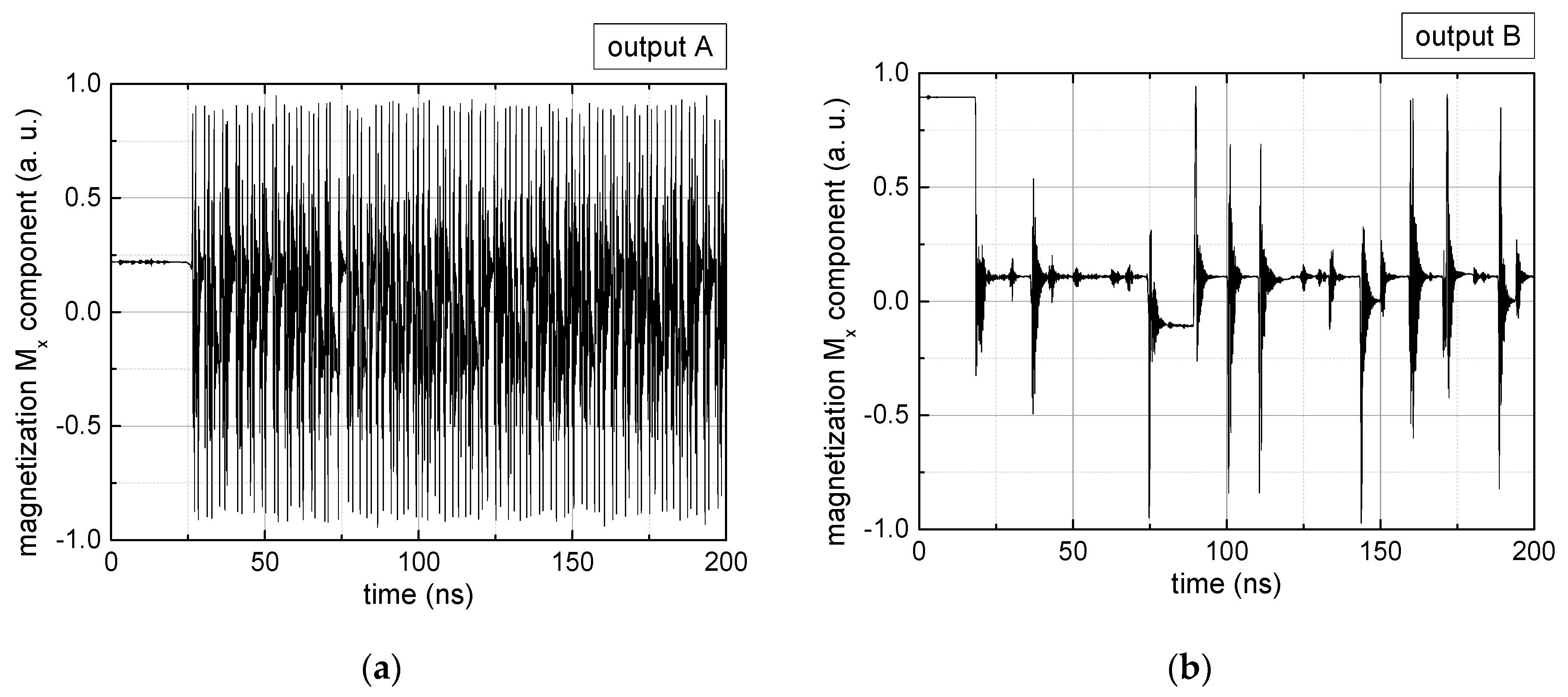
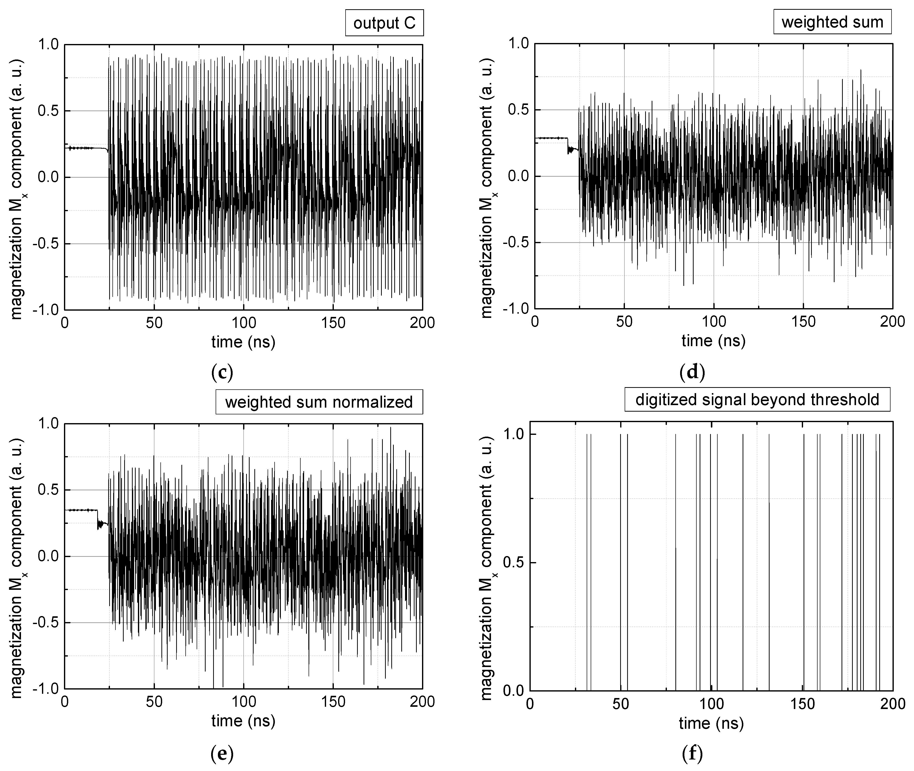
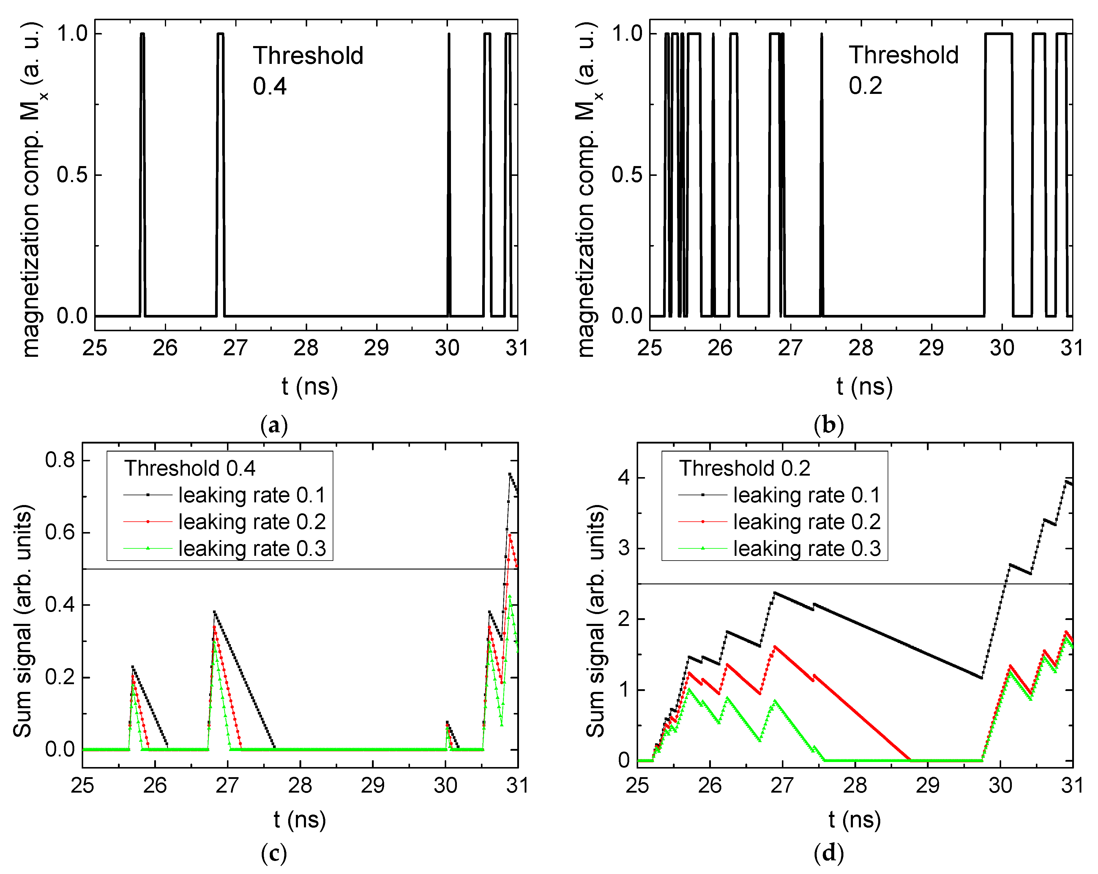
3. Results and Discussion
4. Conclusions
Author Contributions
Funding
Institutional Review Board Statement
Informed Consent Statement
Data Availability Statement
Conflicts of Interest
References
- Jiménez-Fernández, A.; Jimenez-Moreno, G.; Linares-Barranco, A.; Dominguez-Morales, M.J.; Paz-Vicente, R.; Civit-Balcells, A. a neuro-inspired spike-based pid motor controller for multi-motor robots with low Cost fpgas. Sensors 2012, 12, 3831–3856. [Google Scholar] [CrossRef] [PubMed]
- Cerezuela Escudero, E.; Pérez Pena, F.; Paz Vicente, R.; Jimenez-Fernandez, A.; Jimenez Moreno, G.; Morgado-Estevez, A. Real-time neuro-inspired sound source localization and tracking architecture applied to a robotic platform. Neurocomputing 2018, 283, 129–139. [Google Scholar] [CrossRef]
- Dominguez-Morales, M.; Domínguez-Morales, J.P.; Jiménez-Fernández, Á.; Linares-Barranco, A.; Jiménez-Moreno, G. Stereo Matching in Address-Event-Representation (AER) bio-inspired binocular systems in a Field-Programmable Gate Array (FPGA). Electrons 2019, 8, 410. [Google Scholar] [CrossRef]
- Prashanth, B.; Ahmed, M.R. FPGA Implementation of bio-inspired computing architecture based on simple neuron model. In Proceedings of the 2020 International Conference on Artificial Intelligence and Signal Processing (AISP), Amaravati, India, 10–12 January 2020; pp. 1–6. [Google Scholar]
- Locatelli, N.; Grollier, J.; Querlioz, D.; Vincent, A.F.; Mizrahi, A.; Friedman, J.S.; Vodenicarevic, D.; Kim, J.-V.; Klein, J.-O.; Zhao, W. Spintronic devices as key elements for energy-efficient neuroinspired architectures. Des. Automat. Test. Eur. Conf. Exhib. 2015, 2015, 994–999. [Google Scholar]
- Sengupta, A.; Roy, K. Neuromorphic computing enabled by physics of electron spins: Prospects and perspectives. Appl. Phys. Express 2018, 11, 030101. [Google Scholar] [CrossRef]
- Resch, S.; Khatamifard, S.K.; Chowdhury, Z.I.; Zabihi, M.; Zhao, Z.Y.; Wang, J.-P.; Sapatnekar, S.S.; Karpuzcu, U.R. PIMBALL: Binary neural networks in spintronic memory. ACM Transac. Architect. Code Optim. 2019, 16, 41. [Google Scholar] [CrossRef]
- Zhang, W.; Mazzarello, R.; Wuttig, M.; Ma, E. Designing crystallization in phase-change materials for universal memory and neuro-inspired computing. Nat. Rev. Mater. 2019, 4, 150–168. [Google Scholar] [CrossRef]
- Wang, Q.; Niu, G.; Ren, W.; Wang, R.; Chen, X.; Li, X.; Ye, Z.; Xie, Y.; Song, S.; Song, Z. Phase change random access memory for neuro-inspired computing. Adv. Electron. Mater. 2021, 2001241. [Google Scholar] [CrossRef]
- Prashanth, B.U.V.; Ahmed, M.R. Design and performance analysis of artificial neural network based artificial synapse for bio-inspired computing. In Advances in Intelligent Systems and Computing; Springer: Berlin/Heidelberg, Germany, 2020; Volume 1108, pp. 1294–1302. [Google Scholar]
- Richhariya, B.; Tanveer, M. EEG signal classification using universum support vector machine. Expert Syst. Appl. 2018, 106, 169–182. [Google Scholar] [CrossRef]
- Soriano, M.C.; Brunner, D.; Escalona-Morãn, M.; Mirasso, C.; Fischer, I. Minimal approach to neuro-inspired information processing. Front. Comput. Neurosci. 2015, 9, 68. [Google Scholar] [CrossRef]
- Huang, G.; Huang, G.-B.; Song, S.; You, K. Trends in extreme learning machines: A review. Neural Netw. 2015, 61, 32–48. [Google Scholar] [CrossRef] [PubMed]
- Ertuğrul, Ö.F. A novel randomized machine learning approach: Reservoir computing extreme learning machine. Appl. Soft Comput. 2020, 94, 106433. [Google Scholar] [CrossRef]
- Lukoševičius, M.; Jaeger, H.; Schrauwen, B. Reservoir computing trends. KI Künstliche Intell. 2012, 26, 365–371. [Google Scholar] [CrossRef]
- Tanaka, G.; Yamane, T.; Héroux, J.B.; Nakane, R.; Kanazawa, N.; Takeda, S.; Numata, H.; Nakano, D.; Hirose, A. Recent advances in physical reservoir computing: A review. Neural Netw. 2019, 115, 100–123. [Google Scholar] [CrossRef]
- Wong, H.-S.P.; Salahuddin, S. Memory leads the way to better computing. Nat. Nanotechnol. 2015, 10, 191–194. [Google Scholar] [CrossRef] [PubMed]
- Wu, C.; Kim, T.W.; Choi, H.Y.; Strukov, D.B.; Yang, J.J. Flexible three-dimensional artificial synapse networks with correlated learning and trainable memory capability. Nat. Commun. 2017, 8, 1–9. [Google Scholar] [CrossRef]
- Feng, X.; Li, Y.; Wang, L.; Chen, S.; Yu, Z.G.; Tan, W.C.; Macadam, N.; Hu, G.; Huang, L.; Chen, L.; et al. A fully printed flexible mos 2 memristive artificial synapse with femtojoule switching energy. Adv. Electron. Mater. 2019, 5, 1900740. [Google Scholar] [CrossRef]
- Allwood, D.A.; Vernier, N.; Xiong, G.; Cooke, M.D.; Atkinson, D.; Faulkner, C.C.; Cowburn, R. Shifted hysteresis loops from magnetic nanowires. Appl. Phys. Lett. 2002, 81, 4005–4007. [Google Scholar] [CrossRef]
- Cowburn, R.P.; Allwood, D.A.; Xiong, G.; Cooke, M.D. Domain wall injection and propagation in planar Permalloy nanowires. J. Appl. Phys. 2002, 91, 6949. [Google Scholar] [CrossRef]
- Allwood, D.A.; Xiong, G.; Cowburn, R. Domain wall cloning in magnetic nanowires. J. Appl. Phys. 2007, 101, 24308. [Google Scholar] [CrossRef]
- Grollier, J.; Querlioz, D.; Stiles, M.D. Spintronic nanodevices for bioinspired computing. Proc. IEEE 2016, 104, 2024–2039. [Google Scholar] [CrossRef]
- Lequeux, S.; Sampaio, J.; Cros, V.; Yakushiji, K.; Fukushima, A.; Matsumoto, R.; Kubota, H.; Yuasa, S.; Grollier, J. A magnetic synapse: Multilevel spin-torque memristor with perpendicular anisotropy. Sci. Rep. 2016, 6, 31510. [Google Scholar] [CrossRef] [PubMed]
- Ryu, K.-S.; Thomas, L.; Yang, S.-H.; Parkin, S.S.P. Current induced tilting of domain walls in high velocity motion along perpendicularly magnetized micron-sized Co/Ni/Co racetracks. Appl. Phys. Express 2012, 5, 093006. [Google Scholar] [CrossRef]
- Yang, S.-H.; Ryu, K.-S.; Parkin, S.S.P. Domain-wall velocities of up to 750 m s−1 driven by exchange-coupling torque in syn-thetic antiferromagnets. Nat. Nanotechnol. 2015, 10, 221–226. [Google Scholar] [CrossRef] [PubMed]
- Alejos, O.; Raposo, V.; Sanchez-Tejerina, L.; Martinez, E. Efficient and controlled domain wall nucleation for magnetic shift registers. Sci. Rep. 2017, 7, 11909. [Google Scholar] [CrossRef] [PubMed]
- Garg, C.; Yang, S.-H.; Phung, T.; Pushp, A.; Parkin, S.S.P. Dramatic influence of curvature of nanowire on chiral domain wall velocity. Sci. Adv. 2017, 3, e1602804. [Google Scholar] [CrossRef] [PubMed]
- Blachowicz, T.; Ehrmann, A. Magnetization reversal in bent nanofibers of different cross sections. J. Appl. Phys. 2018, 124, 152112. [Google Scholar] [CrossRef]
- Kern, P.; Döpke, C.; Blachowicz, T.; Steblinski, P.; Ehrmann, A. Magnetization reversal in ferromagnetic Fibonacci nano-spirals. J. Magn. Magn. Mater. 2019, 484, 37–41. [Google Scholar] [CrossRef]
- Blachowicz, T.; Döpke, C.; Ehrmann, A. Micromagnetic simulations of chaotic ferromagnetic nanofiber networks. Nanomaterials 2020, 10, 738. [Google Scholar] [CrossRef]
- Pérez-Peña, F.; Morgado-Estevez, A.; Linares-Barranco, A.; Jiménez-Fernández, A.; Gomez-Rodriguez, F.; Jimenez-Moreno, G.; López-Coronado, J. Neuro-Inspired Spike-based motion: From dynamic vision sensor to robot motor open-loop control through Spike-VITE. Sensors 2013, 13, 15805–15832. [Google Scholar] [CrossRef]
- Susi, G.; Toro, L.A.; Canuet, L.; López, M.E.; Maestu, F.; Mirasso, C.R.; Pereda, E. A neuro-inspired system for online learning and recognition of parallel spike trains, based on spike latency, and heterosynaptic STDP. Front. Neurosci. 2018, 12, 780. [Google Scholar] [CrossRef] [PubMed]
- Zhang, W.; Gao, B.; Tang, J.; Yao, P.; Yu, S.; Chang, M.-F.; Yoo, H.-J.; Qian, H.; Wu, H. Neuro-inspired computing chips. Nat. Electron. 2020, 3, 371–382. [Google Scholar] [CrossRef]
- Van de Burgt, Y.; Lubberman, E.; Fuller, E.J.; Keene, S.T.; Faria, G.C.; Agarwal, S.; Marinela, M.J.; Talin, A.A.; Salleo, A. A non-volatile organic electrochemical device as a low-voltage artificial synapse for neuromorphic computing. Nat. Mater. 2017, 16, 414–418. [Google Scholar] [CrossRef] [PubMed]
- Lv, Z.; Zhou, Y.; Han, S.-T.; Roy, V. From biomaterial-based data storage to bio-inspired artificial synapse. Mater. Today 2018, 21, 537–552. [Google Scholar] [CrossRef]
- Tian, B.; Liu, L.; Yan, M.; Wang, J.L.; Zhao, Q.B.; Zhong, N.; Xiang, P.H.; Sun, L.; Peng, H.; Shen, H.; et al. A robust artificial synapse based on organic ferroelectric polymer. Adv. Electron. Mater. 2019, 5, 1800600. [Google Scholar] [CrossRef]
- Scholz, W.; Fidler, J.; Schrefl, T.; Suess, D.; Dittrich, R.; Forster, H.; Tsiantos, V. Scalable parallel micromagnetic solvers for magnetic nanostructures. Comput. Mater. Sci. 2003, 28, 366–383. [Google Scholar] [CrossRef]
- Blachowicz, T.; Ehrmann, A. Spintronics—Theory, Modelling, Devices; De Gruyter: Berlin/Heidelberg, Germany, 2019. [Google Scholar]
- Enrico, A.; Dubois, V.; Niklaus, F.; Stemme, G. Scalable manufacturing of single nanowire devices using crack-defined shadow mask lithography. ACS Appl. Mater. Interfaces 2019, 11, 8217–8226. [Google Scholar] [CrossRef]
- Mun, J.H.; Cha, S.K.; Kim, Y.C.; Yun, T.; Choi, Y.J.; Jin, H.M.; Lee, J.E.; Jeon, H.U.; Kim, S.Y.; Kim, S.O. Controlled segmentation of metal nanowire array by block copolymer lithography and reversible ion loading. Small 2017, 13, 1603939. [Google Scholar] [CrossRef] [PubMed]
- Askey, J.; Hunt, M.O.; Langbein, W.; Ladak, S. Use of two-photon lithography with a negative resist and processing to realise cylindrical magnetic nanowires. Nanomaterials 2020, 10, 429. [Google Scholar] [CrossRef] [PubMed]
- Davies, C.S.; Kruglyak, V.V. Generation of propagating spin waves from edges of magnetic nanostructures pumped by uniform microwave magnetic field. IEEE Trans. Magn. 2016, 52, 1–4. [Google Scholar] [CrossRef]
- Gruszecki, P.; Kasprzak, M.; Serebryannikov, A.E.; Krawczyk, M.; Śmigaj, W. Microwave excitation of spin wave beams in thin ferromagnetic films. Sci. Rep. 2016, 6, 22367. [Google Scholar] [CrossRef] [PubMed]
- Mushenok, F.B.; Dost, R.; Davies, C.S.; Allwood, D.A.; Inkson, B.J.; Hrkac, G.; Kruglyak, V.V. Broadband conversion of microwaves into propagating spin waves in patterned magnetic structures. Appl. Phys. Lett. 2017, 111, 042404. [Google Scholar] [CrossRef]
- Haldar, A.; Adeyeye, A.O. Microwave assisted gating of spin wave propagation. Appl. Phys. Lett. 2020, 116, 162403. [Google Scholar] [CrossRef]
- Hoppensteadt, F. Spin torque oscillator neuroanalog of von Neumann’s microwave computer. Biosystems 2015, 136, 99–104. [Google Scholar] [CrossRef] [PubMed]
- Blachowicz, T.; Ehrmann, A. Magnetic elements for neuromorphic computing. Molecules 2020, 25, 2550. [Google Scholar] [CrossRef] [PubMed]
- Sengupta, A.; Roy, K. Encoding neural and synaptic functionalities in electron spin: A pathway to efficient neuromorphic computing. Appl. Phys. Rev. 2017, 4, 041105. [Google Scholar] [CrossRef]


| 0.8 |  |  |  |
| 0.4 |  |  |  |
| 0 |  |  |  |
| −0.4 |  |  |  |
| −0.8 |  |  |  |
| Mth | LL | LR | RL | RR |
|---|---|---|---|---|
| +0.8 | 0.0032 | 0.0022 | 0.0015 | 0.0008 |
| +0.4 | 0.0487 | 0.0591 | 0.0681 | 0.0809 |
| 0.0 | 0.3010 | 0.4839 | 0.5593 | 0.3169 |
| −0.4 | 0.9867 | 0.9330 | 0.9452 | 0.9839 |
| −0.8 | 0.9997 | 0.9985 | 0.9981 | 1.0000 |
| Mth | LL | LR | RL | RR |
|---|---|---|---|---|
| +0.8 | 0.0010 | 0.0022 | 0.0021 | 0.0019 |
| +0.4 | 0.1431 | 0.0607 | 0.1426 | 0.1976 |
| 0.0 | 0.5754 | 0.4820 | 0.5754 | 0.8356 |
| −0.4 | 0.9750 | 0.9286 | 0.9495 | 0.9982 |
| −0.8 | 0.9993 | 0.9980 | 0.9987 | 1.0000 |
| Mth | LL | LR | RL | RR |
|---|---|---|---|---|
| +0.8 | 0.0062 | 0.0018 | 0.0013 | 0.0032 |
| +0.4 | 0.1630 | 0.0526 | 0.1226 | 0.3047 |
| 0.0 | 0.4832 | 0.4811 | 0.5940 | 0.9532 |
| −0.4 | 0.9999 | 0.9365 | 0.9704 | 1.0000 |
| −0.8 | 1.0000 | 0.9989 | 0.9999 | 1.0000 |
Publisher’s Note: MDPI stays neutral with regard to jurisdictional claims in published maps and institutional affiliations. |
© 2021 by the authors. Licensee MDPI, Basel, Switzerland. This article is an open access article distributed under the terms and conditions of the Creative Commons Attribution (CC BY) license (https://creativecommons.org/licenses/by/4.0/).
Share and Cite
Blachowicz, T.; Grzybowski, J.; Steblinski, P.; Ehrmann, A. Neuro-Inspired Signal Processing in Ferromagnetic Nanofibers. Biomimetics 2021, 6, 32. https://doi.org/10.3390/biomimetics6020032
Blachowicz T, Grzybowski J, Steblinski P, Ehrmann A. Neuro-Inspired Signal Processing in Ferromagnetic Nanofibers. Biomimetics. 2021; 6(2):32. https://doi.org/10.3390/biomimetics6020032
Chicago/Turabian StyleBlachowicz, Tomasz, Jacek Grzybowski, Pawel Steblinski, and Andrea Ehrmann. 2021. "Neuro-Inspired Signal Processing in Ferromagnetic Nanofibers" Biomimetics 6, no. 2: 32. https://doi.org/10.3390/biomimetics6020032
APA StyleBlachowicz, T., Grzybowski, J., Steblinski, P., & Ehrmann, A. (2021). Neuro-Inspired Signal Processing in Ferromagnetic Nanofibers. Biomimetics, 6(2), 32. https://doi.org/10.3390/biomimetics6020032