1. Introduction
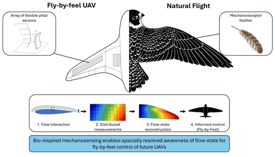
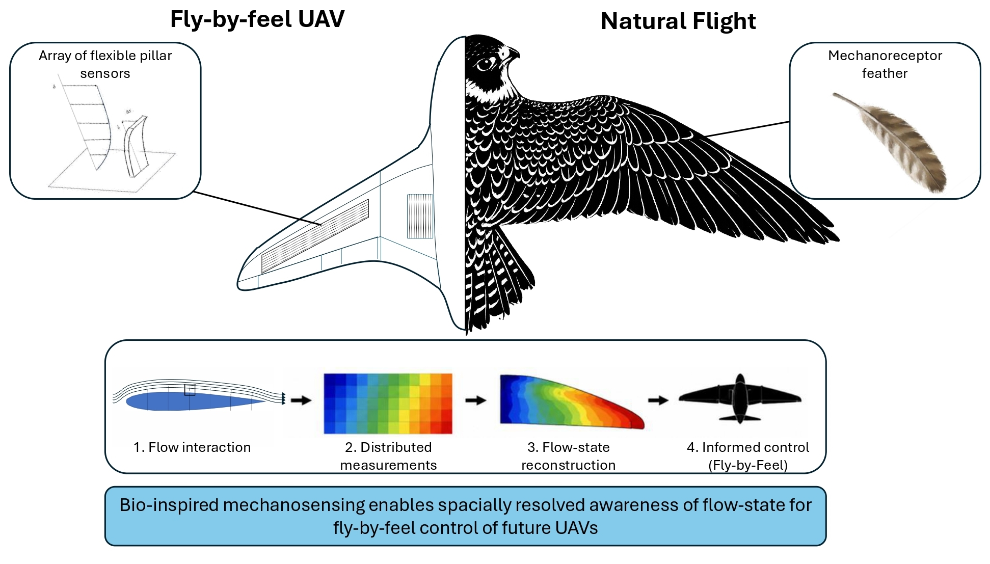
Natural fliers rely extensively on distributed mechanosensory systems to perceive local aerodynamic conditions during flight. These systems frequently employ compliant sensing structures whose deformation under aerodynamic loading provides continuous information regarding the surrounding flow environment. Inspired by such biological sensing architectures, biomimetic adaptations of such sensing principles are seen in engineered systems such as within strain gauges, load cells, and pressure sensors, where flexible elements embedded within the systems to deform due to loads are essential to sense and report on the intended quantities. In practice, the known material properties of a certain element allow a repeatable and deterministic response to stimulus, which is subsequently used to quantify the magnitude and direction of the stimulus, whether arising from bodily interactions such as applied forces or dynamic factors like fluid velocity.
Flexible element sensors are commonly found present in a variety of flying animal species through different domains. Particularly on the wings of bats, it is seen that the wings are covered with rows of microscopic flexible wind-hairs arranged in grids [
1,
2], which serve a mechanoreceptor purpose to inform flight control. Earlier work investigated the mechanoreceptors in covert feathers of various bird species which were also seen to provide sensory information to aid flight efficiency and stability [
3,
4]. These same principles are observed in insect flight, with the difference of scales and sensor types [
5,
6], and it was found in [
7] that such sensors have capabilities to add the sensing of structural geometric changes within the wing in addition to flow information, further informing the system. Mechanosensation in flying animals typically requires not only the capability to sense mechanical forces themselves [
8], but also to be able to ascertain trends in differential forces from the baseline [
9]. An example of this is seen particularly in fast-flying birds of prey. It was seen in Peregrine falcons that there exist specific mechanoreceptor dorsal feathers responsible for sensing changes in the frequency domain which inform the bird on flight attitudes and angle of attack [
10], an important flight characteristic which allows the bird to fly at marginal stability to achieve superior agility and maneuverability in hunting [
11].
The development of the sensors discussed herein was inspired by the nature of biological sensing to be a distributed, robust, and redundant system of sensors, typically providing multimodal environmental information [
12]. The design and development and the results of preliminary tests in air are discussed in [
13,
14] where it is shown how a single row of sensors placed at specific locations and patterns can provide spatially distributed aerodynamic information toward enabling fly-by-feel flow-state awareness. The flexible pillar sensors were designed and fabricated in-house and are identical to those developed and characterised in [
13,
14]. The sensors do not transmit signals through internal wiring but, instead, the fluorescent-coated tips are tracked optically via wavelength-filtered high-speed imaging of tip deflection, enabling remote, distributed non-intrusive flow-state sensing. Careful in situ calibration and dynamic testing was carried out in the studies included herein which were similar to the methods outlined in [
14]. Underwater tests monitoring the deflection of whiskers using similar techniques as those used within this study are shown in [
15] where a deep learning algorithm was developed and integrated to locate upstream obstacles. Optical monitoring of flexible structures was shown in [
16] where similar optically monitored elastic sensors were used to quantify the wall shear stress in an aortic heart valve model, demonstrating the versatility provided by the use of biologically inspired systems with distributed compliant, non-contact, optical sensing. The relative size of the sensors dictates the sensitivity to changes in the local boundary layer characteristics [
17], which allows the monitoring of the spatial evolution of the boundary layer over various geometries. Recent advances in bio-inspired aerodynamic sensing have highlighted the growing potential of distributed flow-sensitive mechanoreceptive systems for flight-state awareness and flow event detection [
18]. Unlike distributed biological sensing systems, conventional UAV aerodynamic sensing frequently relies on isolated point measurements, whereas more advanced systems such as laser Doppler velocimetry (LDV) can provide highly precise flow measurement [
19], particularly for physically restrictive geometrical constraints. However, these require coherent light sources, sensitive alignment, and are costly and impractical for small UAV deployment.
Previous work on distributed strain and airflow sensing for UAV flight control has similarly demonstrated the advantages of distributed aerodynamic sensing over conventional rigid-body state estimation approaches [
20]. The approach presented herein explores distributed surface-based aerodynamic sensing through passive compliant sensing elements and low-cost imaging, toward enabling distributed fly-by-feel aerodynamic perception for UAV systems.
Herein, the results from tests of a flexible element sensor developed to provide distributed flow measurements in various single-phase flows are presented and analysed. The novelty of this study is showcasing the concept of implementing real-time distributed detection of stall-related flow phenomena using an optically tracked flexible pillar sensor array on an aerofoil. The tests presented are intended to expand on the results from [
14], where a single row of flexible sensors was tested in a wind tunnel on an NACA0012 symmetric aerofoil, a widely used benchmark geometry in aerodynamic research, to determine their capability to perceive evolving aerodynamic conditions and their ability to characterise specific pre-stall phenomena. The NACA0012 aerofoil was deliberately chosen as a canonical, well-documented profile to allow comparison with a wide body of existing literature and to isolate stall-related flow features in a controlled setting. While the simplicity of the geometry limits generalisation, this study serves as a foundational step toward future bio-inspired aerodynamic sensing and adaptive flight control systems. In particular, the tests reported herein were carried out in a water-tunnel environment (
Figure 1) in an effort to achieve the following objectives. Primarily, the water-tunnel tests were carried out to facilitate high-resolution flow visualisation and time-resolved PIV measurements while maintaining chord-based Reynolds numbers representative of small- to medium-scale UAV flight conditions. The lower flow velocities achievable in water enabled detailed observation of the interaction between the distributed pillar array and the surrounding flow field. The conditions for the tests are discussed in detail further in the paper and the differences are highlighted between the underwater tests and tests carried out in air, particularly on the dynamic response of the pillar sensors. Tests were also carried out to measure the distributed sensor interaction effects, in addition to examining the results of arranging the sensors in an array, exploring their response to localised aerodynamic disturbances, such as stall or high turbulence, on a washed-out wing.
2. Materialsand Methods
The results reported herein are of the experimental work carried out in City St. George’s University low-speed water tunnel shown in
Figure 1. The water tunnel is an open-surface, closed loop tunnel, with a transparent test section of 40 × 50 × 120 cm which allows good optical access for both the PIV experiments and the sensor tracking experiments carried out.
2.1. PIV Setup
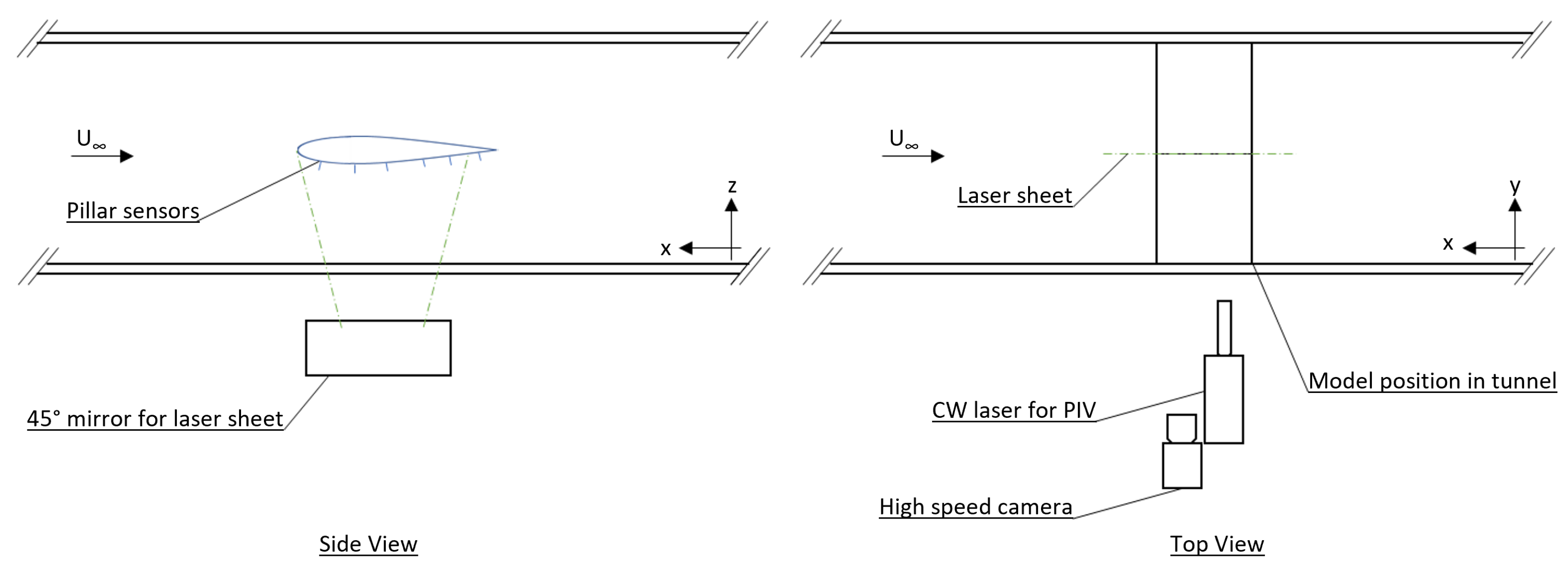
The model was setup to span the width of the tunnel, such that the span axis is parallel to the open surface. A continuous wave Argon-Ion laser (Raypower 5000, Dantec Dynamics, Skovlunde, Denmark, 5 W power at
= 532 nm) was used as an illumination source aligned with a high-speed camera as shown in (
Figure 1). The laser source was positioned in line with and below the camera. A
mirror was placed beneath the tunnel to reorient the beam by
, producing a laser sheet orthogonal to the camera’s optical axis, as illustrated in the figure.
Neutrally buoyant particles (hollow glass spheres, diameter 50 m) were mixed into the fluid and allowed to homogenise before measurements were taken. These seeding particles were introduced specifically for the PIV measurements rather than relying on naturally occurring particles present in the water, which has typically yielded poor correlation due to their irregular shape, variable size, and lack of neutral buoyancy. The controlled use of uniformly shaped particles ensured reliable and accurate reconstruction of the velocity field. The resulting seeding concentration produced an average of 7 particles per 32 × 32 pixel interrogation window, consistent with prior work using the same setup.
A Phantom M310 high-speed camera (Adept Turnkey, Perth, Australia) was arranged orthogonally to the laser sheet and fitted with a varifocal lens used at focal lengths of 100 mm and 300 mm for wide-angle and close-in measurements, respectively. The laser sheet thickness was approximately 1 mm. Image sequences were captured at 3000 fps, but every other frame was used in processing, resulting in an effective inter-frame time () of 0.666 ms. This provided a mean particle image displacement of approximately 1.94 pixels per frame.
The field-of-view magnification factor was 0.06. Image processing was performed using PIVLab [
21], employing a standard multi-pass cross-correlation algorithm with sub-pixel Gaussian fitting yielding a velocity uncertainty on the order of
m/s, with sub-pixel displacement uncertainty estimated between 0.03 and 0.05 pixels. The first pass used a 64 × 64 pixels interrogation window, followed by three refinement passes at 32 × 32 pixels with a slight reduction to 30 pixels in the final pass. A 50% overlap (32 pixels step size) was applied. Outlier removal was performed using a standard deviation filter of 8, and a median filter of 3. The calibration factor was determined as 1 pixels = 0.0001 m.
2.2. Sensing Wing Preparation
Work already carried out at City, University of London produced flexible pillar sensors [
14], which act as a bio-inspired surface-mounted sensor array when applied to an aerofoil, representing arrays of biomimetic wind-hairs that sense the flow. The deflection of the pillars scale with the local Reynolds number, as described in [
14], and therefore by employing the pillar sensors within an array along the suction side of the wing, the effect of aerodynamic phenomena on local flow can be detected and quantified.
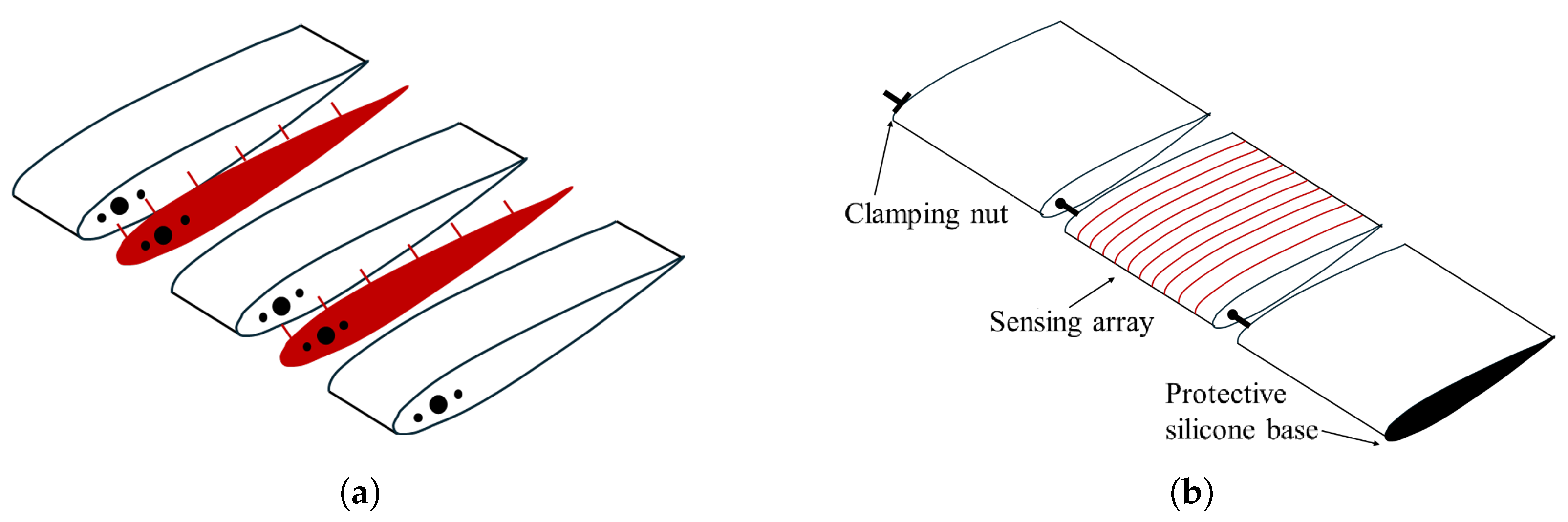
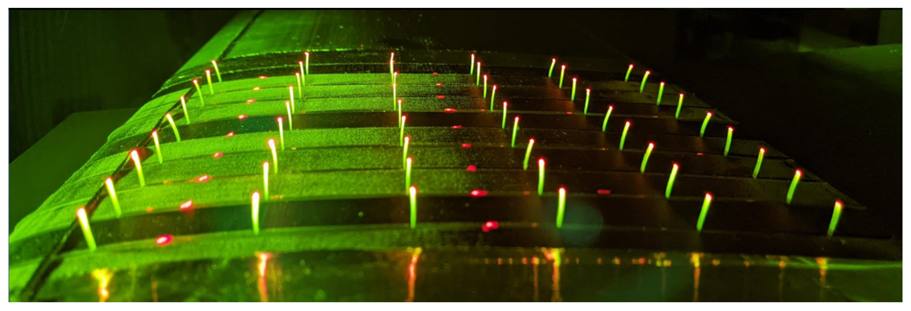
The sensor array was embedded on the suction side of an NACA0012 wing section, as shown in
Figure 2 and
Figure 3. The pillars have the same dimensions as those used in [
14], with a rectangular cross-section measuring 1.5 mm in the spanwise direction and 0.3 mm in the chordwise direction. The array consists of 6 pillars arranged chordwise at 15% chord spacing starting at 15% chord, and 9 rows spaced with 8.6% chord spanwise, forming a
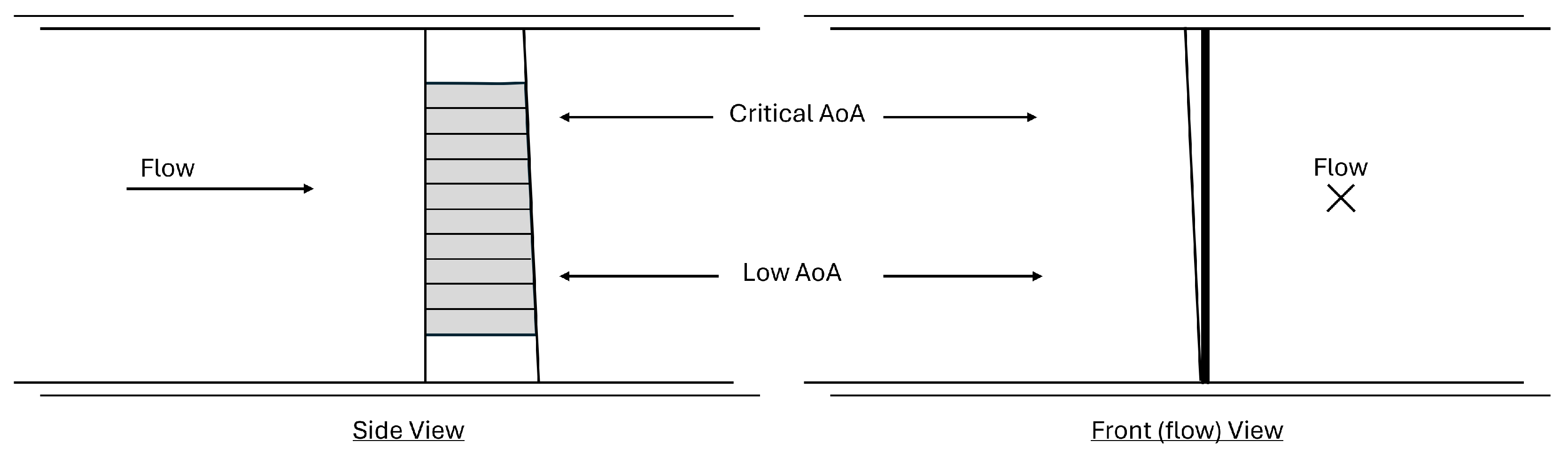
grid of sensors. The wing incorporated a designed washout (twist) across the span. As a result, the local angle of attack at the root (top section) of the wing was higher than that at the tip (lower section), as illustrated in
Figure 4. The wing was placed and adjusted such that the angle of attack experienced by the inboard row of sensors was at a critical pre-stall condition at
angle of attack, with the angle gradually decreasing along the span towards the tip such that the outboard row was at
. This setup was based on known aerofoil characteristics and previous test results, and was validated through preliminary TR-PIV measurements conducted before the main array experiments.
The selected condition provided a controlled spanwise variation in local flow state, placing the inboard section near incipient stall while maintaining attached flow over the outboard section. This enabled the simultaneous observation of attached and pre-stall flow conditions across the sensor array and was considered particularly suitable for investigating boundary layer growth, flow separation, and stall-related phenomena using distributed bio-inspired sensing.
The same optical setup described in
Figure 1 was used, replacing the laser sheet with a wider LED illuminator (IL-105/6X Illuminator, HardSoft, Obergriesbach, Germany) to enhance illumination of the pillar tips.The fluorescent tips were captured at a sampling rate of 1000 Hz and processed using a modified version of an in-house MATLAB-based cross-correlation algorithm (MATLAB Release R2023b), which compares small interrogation windows around the pillar tips to their wind-off position, enabling simultaneous tracking of the full sensor array. The details of this algorithm are further discussed in [
14].
The pillars are laser cut from silicone sheets of thickness 1.5 mm and density 1.2 g/cm
3. Each cut section is an NACA0012 aerofoil cross-section of chord 20 cm and each has 6 pillars at even spacing of 15% chord along the suction side. These sections are then clamped in between 3D-printed aerofoil sections to produce a modular sensing aerofoil, where the pillars act as cantilever beams. The pillars have a rectangular cross-section of 1.5 mm spanwise by 0.3 mm chordwise; these dimensions were chosen to emphasise deflection in the chordwise direction thus providing a clear instantaneous flow picture, with reduced noise from other out of plane motion. The material properties and setup are summarised in
Table 1 and the clamping mechanism is illustrated in
Figure 2.
2.3. Reynolds Number Scaling and UAV Relevance
The experiments were conducted at a chord-based Reynolds number of = 70,000, corresponding to flow conditions representative of the lower end of the flight envelope encountered by small- to medium-scale fixed-wing UAVs, such as launch and recovery, where stall phenomena are more prevalent. The use of a water tunnel enabled these Reynolds numbers to be achieved at substantially lower free-stream velocities than would be required in air, facilitating high-resolution flow visualisation and time-resolved PIV measurements.
The objective of the study was to investigate the ability of distributed flexible pillar sensors to detect flow-state signatures associated with boundary-layer growth, flow separation, flow reversal, and stall onset. These phenomena are governed primarily by the local flow state and Reynolds number. Consequently, the water-tunnel environment provides a suitable platform for investigating the sensing principles considered herein while maintaining flow conditions relevant to small- and medium-scale UAV applications.
2.4. Sensor Calibration
The sensor calibration process for the water-tunnel experiment involved an impulse excitation test on one of the leading edge pillars to determine the physical parameters of the submerged pillars. To establish the velocity calibration, the free-stream velocity was increased incrementally and pillar recordings were taken in the same method as before, and mean values obtained. These were compared to free-stream Particle Image Velocimetry (PIV) measurements to construct a comprehensive velocity curve. This calibration methodology draws parallels to previous work outlined in [
13], with the distinct difference that the velocity in this study is the free-stream velocity, whilst in the previous studies, it was the local velocity. The velocity increments covered the entire range of experimental conditions.
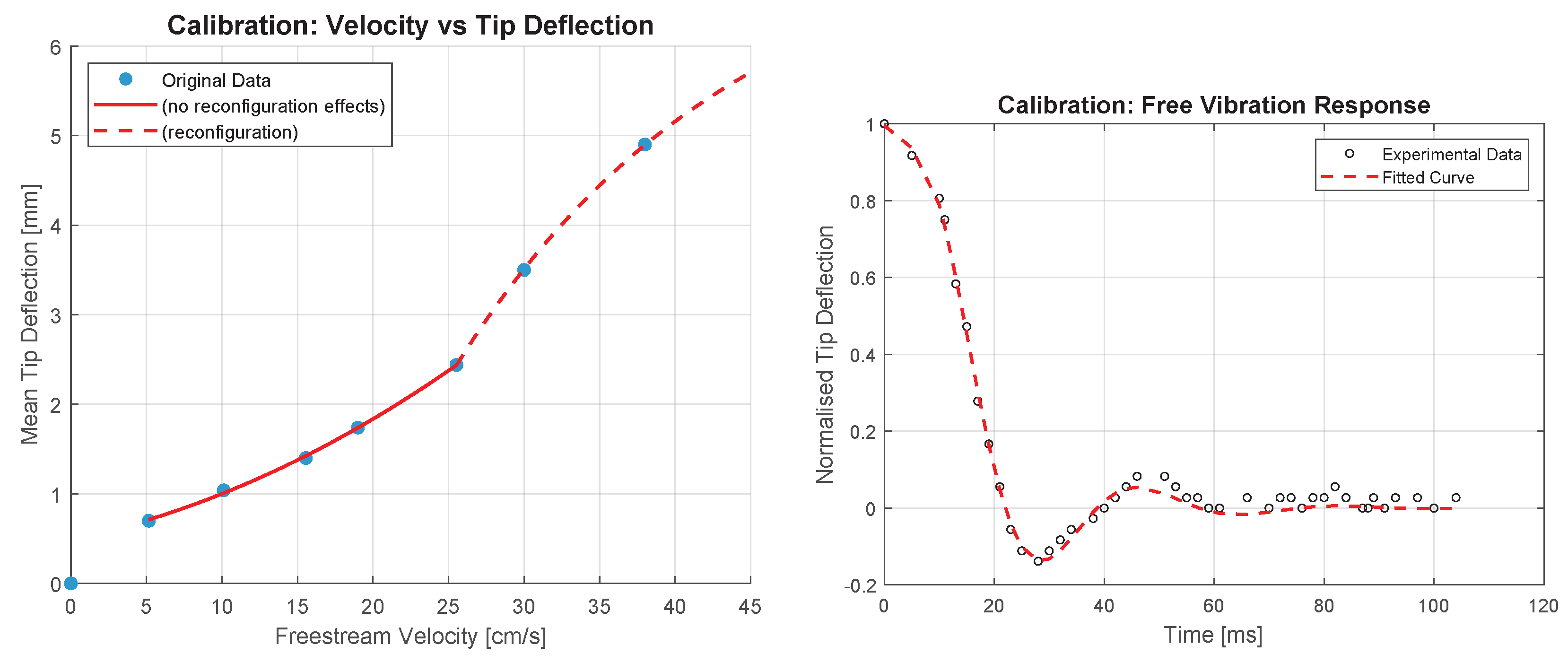
The velocity calibration shown in
Figure 5 was represented using separate fitted relationships below and above the onset of pillar reconfiguration. Prior to reconfiguration, the mean tip deflection was well described by a second-order polynomial fit, while an exponential asymptotic fit was employed above the reconfiguration threshold to account for the reduced sensitivity as the pillar approached its maximum operable deflection. The resulting calibration relation is given by
where
Q is the mean tip deflection in mm,
v is the free-stream velocity in
, and
denotes the onset of reconfiguration. The optical tracking uncertainty was estimated as 0.03–0.05 pixels based on the cross-correlation methodology employed [
22] corresponding to a tip-deflection uncertainty of approximately 0.01 mm which yields an estimated velocity uncertainty below 0.1 cm s
−1 in the most sensitive operating regime. In the low-velocity regime, the sensor exhibited an approximately linear response of
.
Furthermore, dynamic parameters such as natural frequency and damping coefficients were determined through an impulse excitation test, where the pillar was manually deflected to its maximum operable displacement and released, allowing the free-decay motion to be optically tracked. The results of these tests are illustrated in
Figure 5. The first plot shows the relationship between mean tip deflection and free-stream velocity, while the second plot illustrates the normalised damped oscillatory response of a submerged sensor following release from deflection. The purpose of the impulse excitation test was to identify the dominant dynamic response of the sensor. Previous structural analyses of the same pillar geometry reported a dominant first bending mode with substantial frequency separation from higher-order bending and torsional modes [
14]. Although fluid loading in the present submerged configuration reduced the measured natural frequency, the free-decay response was found to be well described by a single underdamped oscillatory mode. Consequently, a linear underdamped second-order representation was considered sufficient for dynamic characterisation. A second-order underdamped model was therefore fitted to the raw free-decay deflection signal, independently of the low-pass filtering procedure later applied to the flow-measurement time histories. The oscillatory response was modelled as
where
A is the initial amplitude,
c is the decay rate,
is the damped natural frequency,
is the phase offset, and
B is a baseline shift. Fitting this model to the normalized deflection signal yielded a damped natural frequency of approximately
, with a decay rate
, and an estimated damping ratio:
The parameters of Equation (
2) were estimated using nonlinear least-squares fitting in MATLAB. The measured free-decay response was normalised by the maximum measured tip deflection, and the model parameters were obtained by minimising the residual error between the measured and fitted deflection. The identified damped natural frequency and damping ratio provide a practical assessment of the sensor dynamics relevant to the present study. The response settled to near-zero amplitude within approximately 60 ms, consistent with the identified second-order dynamics. Since the aerodynamic analysis presented herein focuses on low-frequency flow phenomena below the 5 Hz filtering threshold, the frequencies of interest remain well separated from the dominant structural response of the sensor. These results went on to inform the signal processing and filtration strategy outlined in
Section 3.
4. Discussion
The paper’s results provide some insights into the behaviour and capabilities of the pillar sensors in the water-tunnel test environment. The findings are discussed below along with their implications, potential applications, and limitations of the sensor system.
The calibration was carried out in situ and the sensor response fit to a second-order polynomial fit for velocities above 5 cm/s and up to velocities of 25 cm/s after which the deflection exceeds 30% of the pillar length and thus reconfiguration effects, which is the natural tendency of flexible elements to modulate their drag as they deform [
25], begin to appear. For velocities higher than 25 {cm/s, an exponentially decaying curve was fit that follows the expected behaviour due to reconfiguration effects [
26] similar to what was observed in wind-tunnel tests [
14]. Furthermore, the impulse excitation test provided information about the sensors’ underwater damping parameters and settling time. The calibration was carried out with the purpose of properly interpreting the results from this experiment and would not be appropriate for a different environment or working fluid. Previous work in wind-tunnel experiments showed that both the dynamic and static responses from the pillars differed.
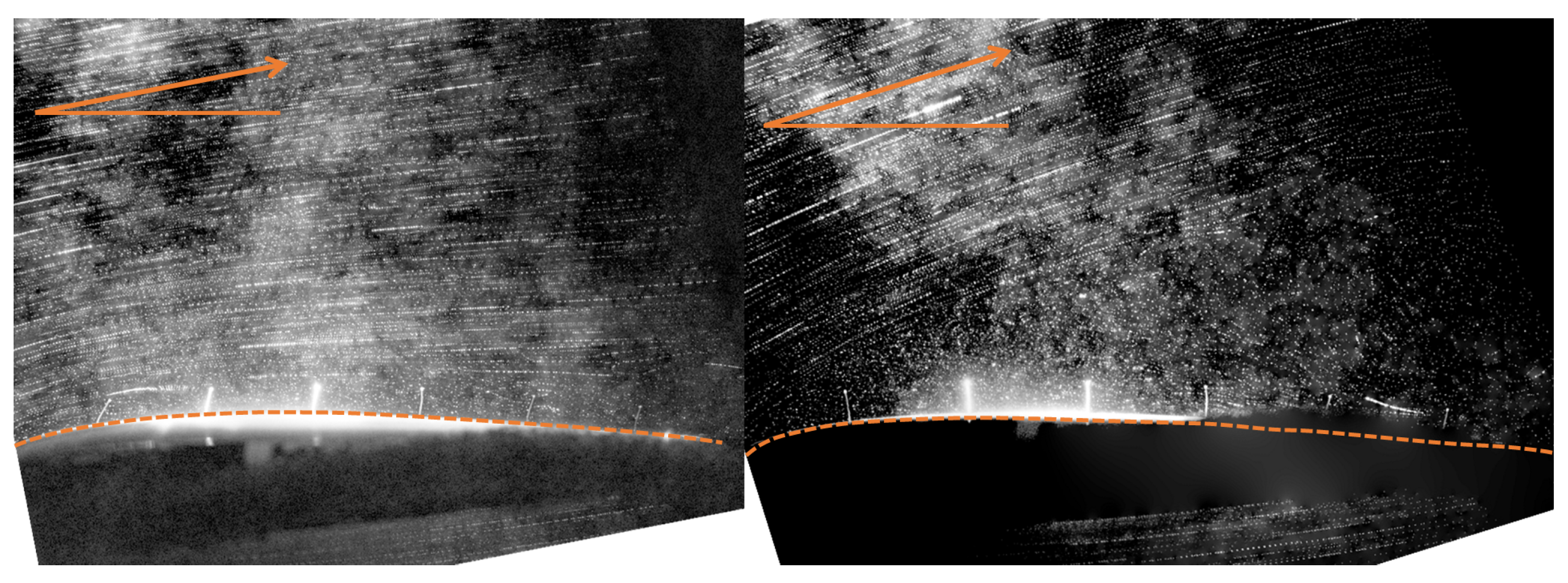
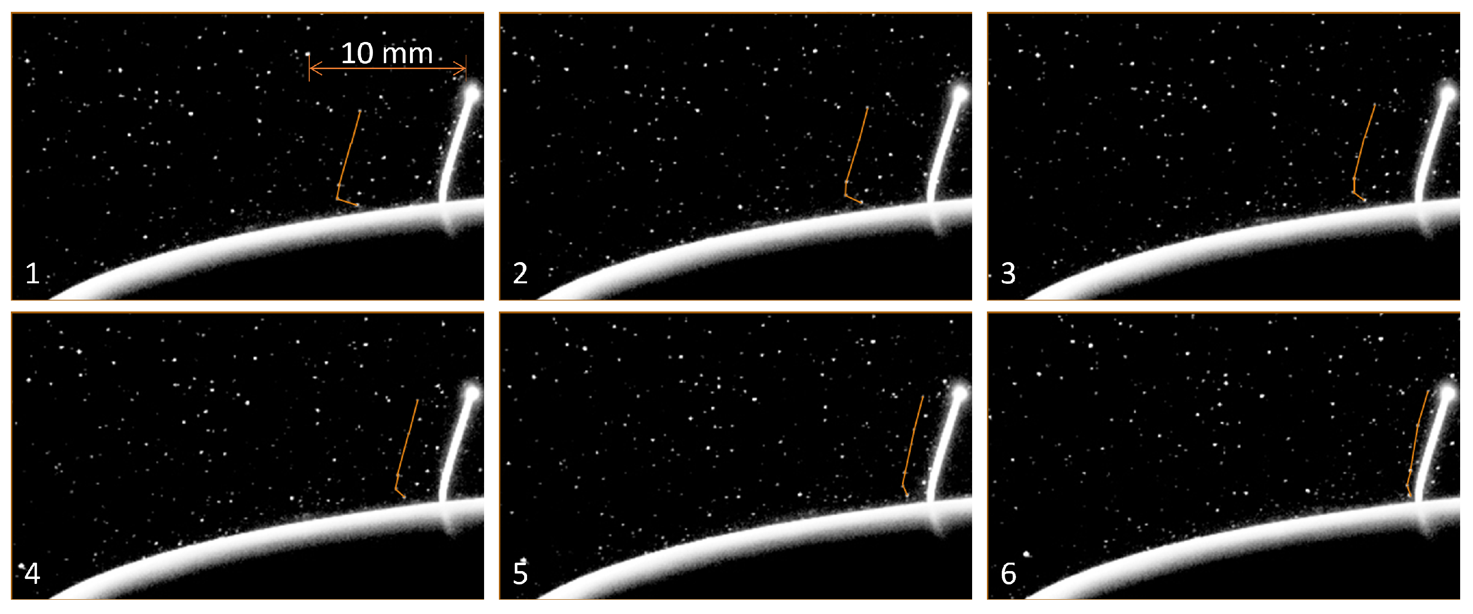
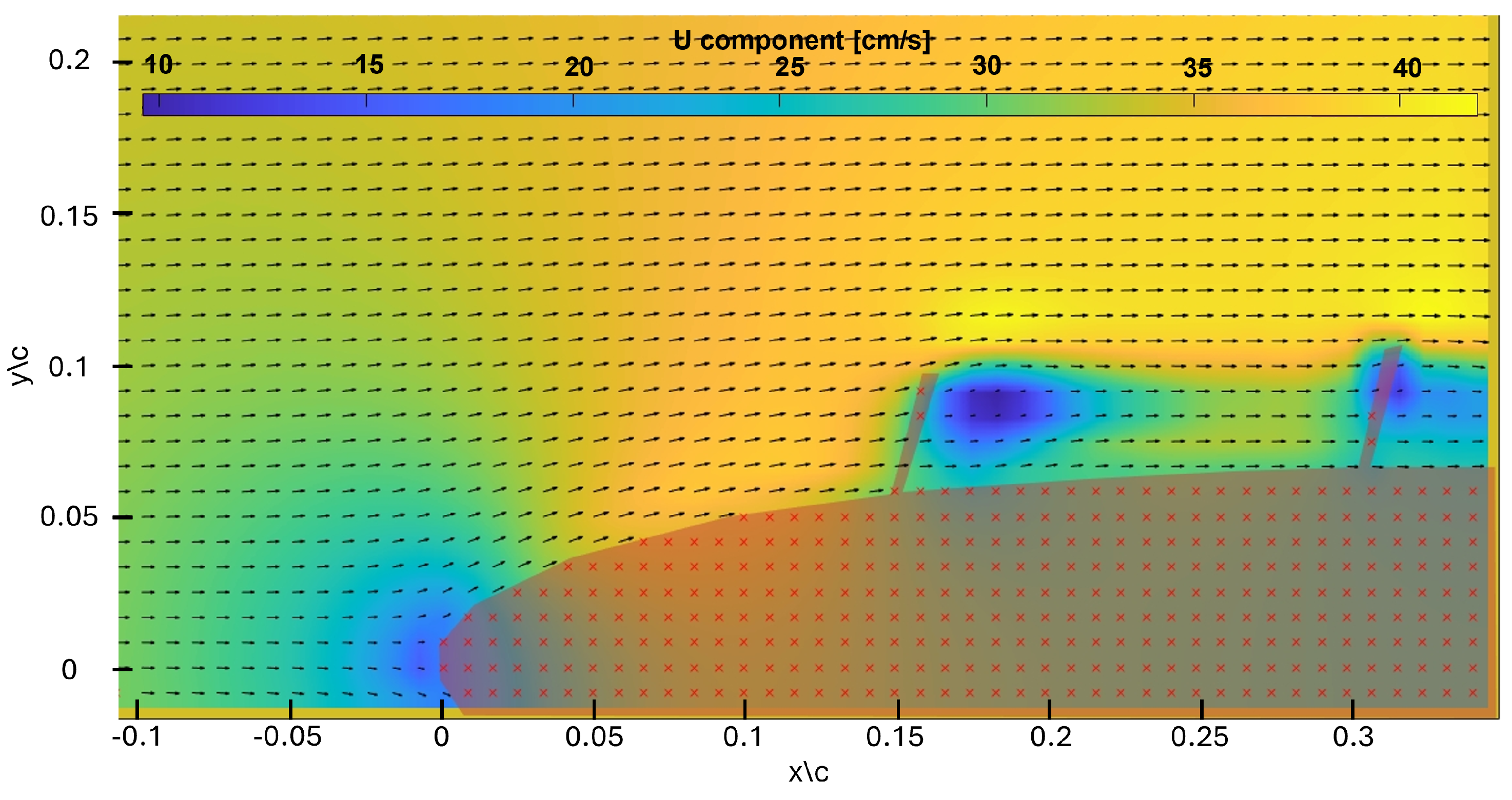
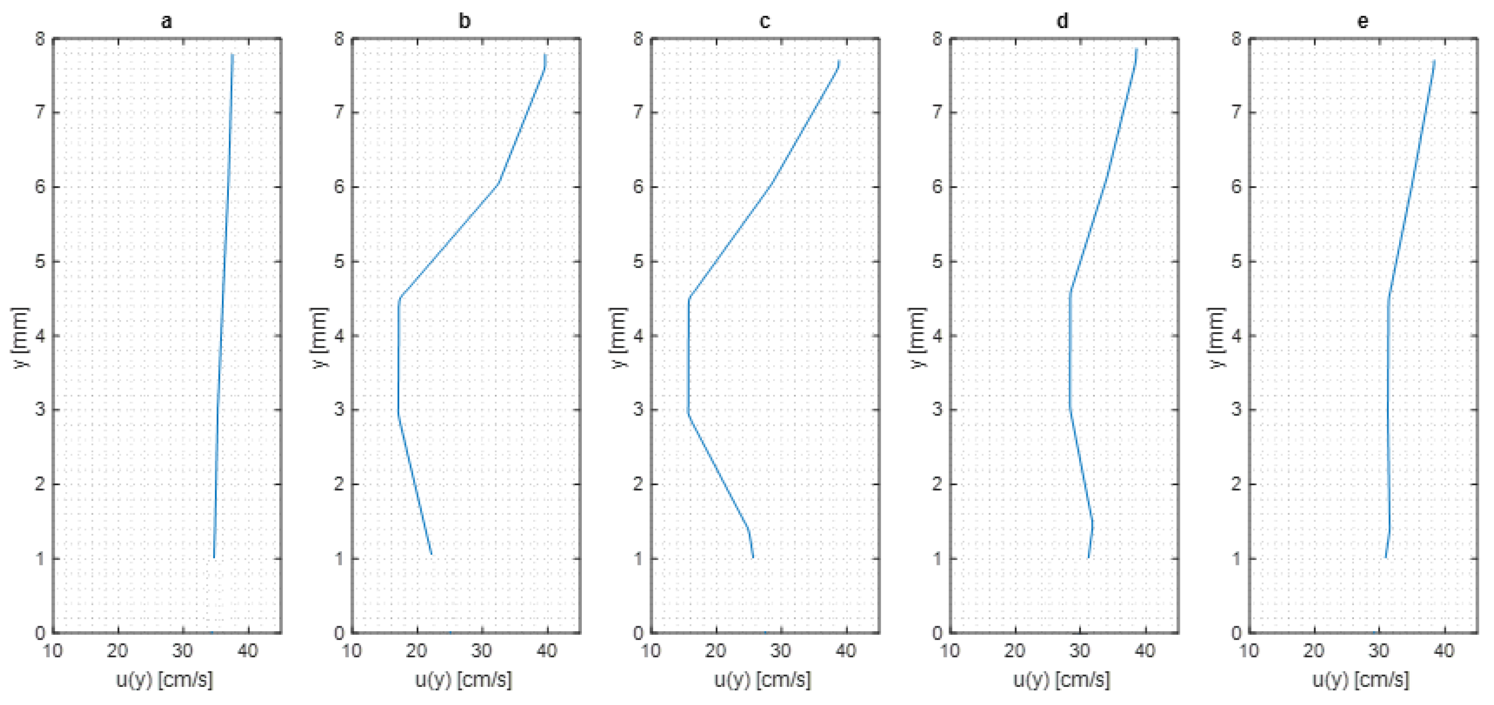
The PIV tests on the leading edge pillars revealed that the boundary layer flow contributes less than 10% of the pillar length at angle of attack rising to at . This indicates that the boundary layer has a negligible effect on the leading edge sensor output at low angles of attack, where that sensor’s response is primarily to bulk flow properties rather than boundary layer characteristics, and that the effects begin to take effect at moderate to high angles of attack. This suggests that further work is required to fully quantify the effect of boundary layer profile and growth on the pillar tip deflection output, in addition to possibly placing the leading edge pillar slightly upstream to reduce the effect.
Moreover, the PIV results showed flow retardation in the immediate wake of the pillar and its gradual reduction further downstream. A probe in the wake showed how the flow retardation decreased from 53% in the immediate wake to 11% 20 major diameters downstream. This suggests that sensors should be placed no fewer than 20 major diameters downstream from one another to mitigate wake-induced vibrations. The visualisations of boundary layer growth helped explain how a separated boundary layer over the sensor would subtract from the deflection and reverse the deflection past the wind-off positions in specific flow conditions. This observation serves as a marker of separated boundary layer and stall.
Tests with an array of the sensors embedded within the suction side of a washed out wing section indicated specific responses that were previously seen to be characteristic of onset flow separation [
14]. These were apparent on the “inboard” section of the wing as would be expected. The observations of
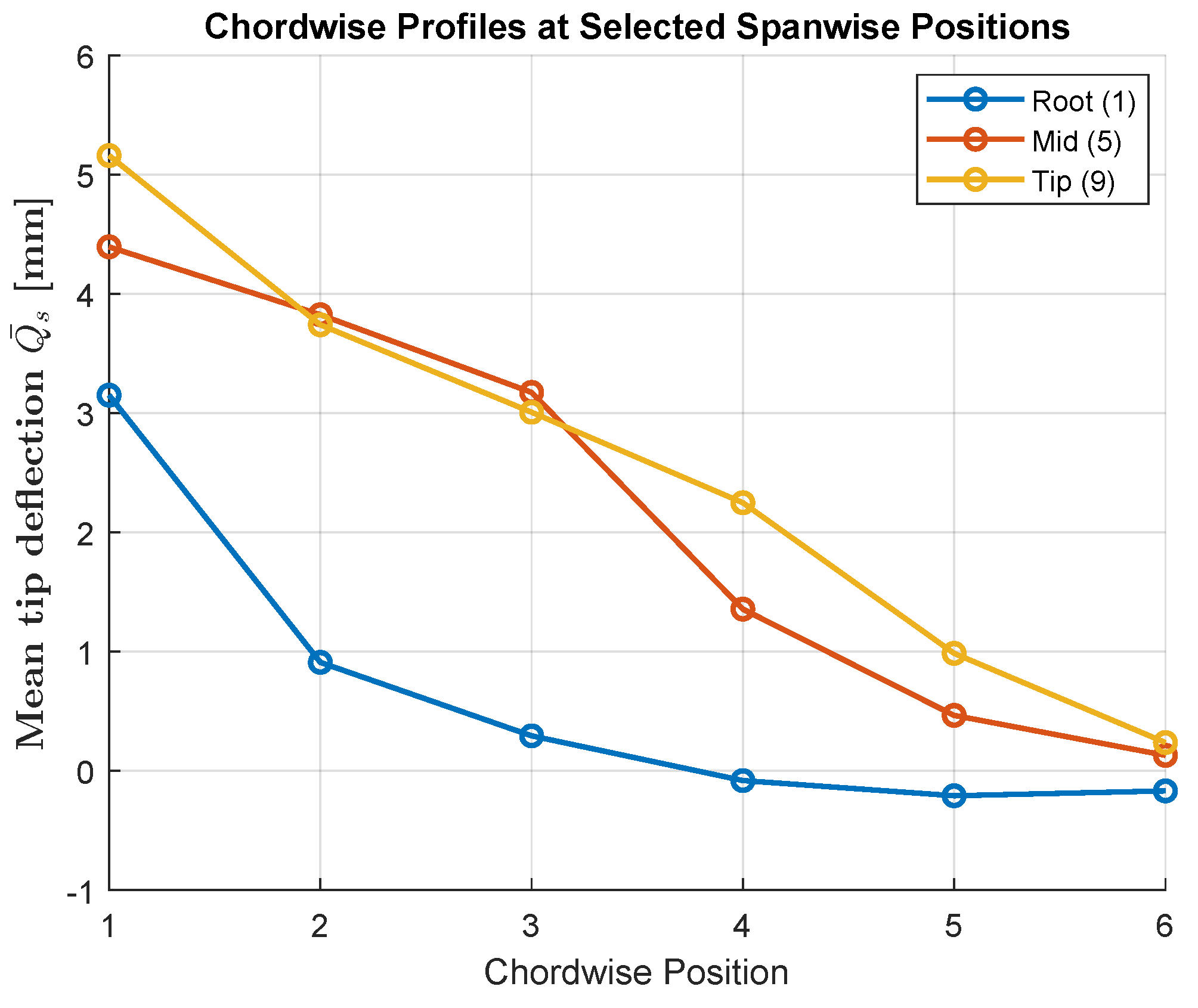
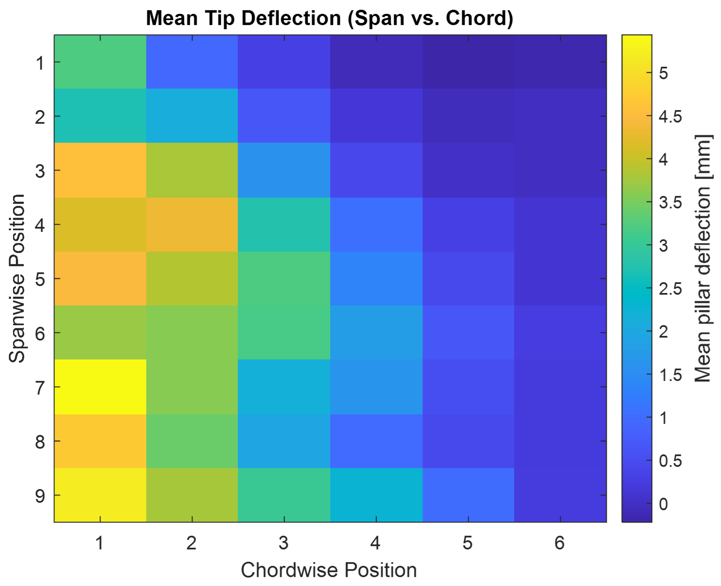
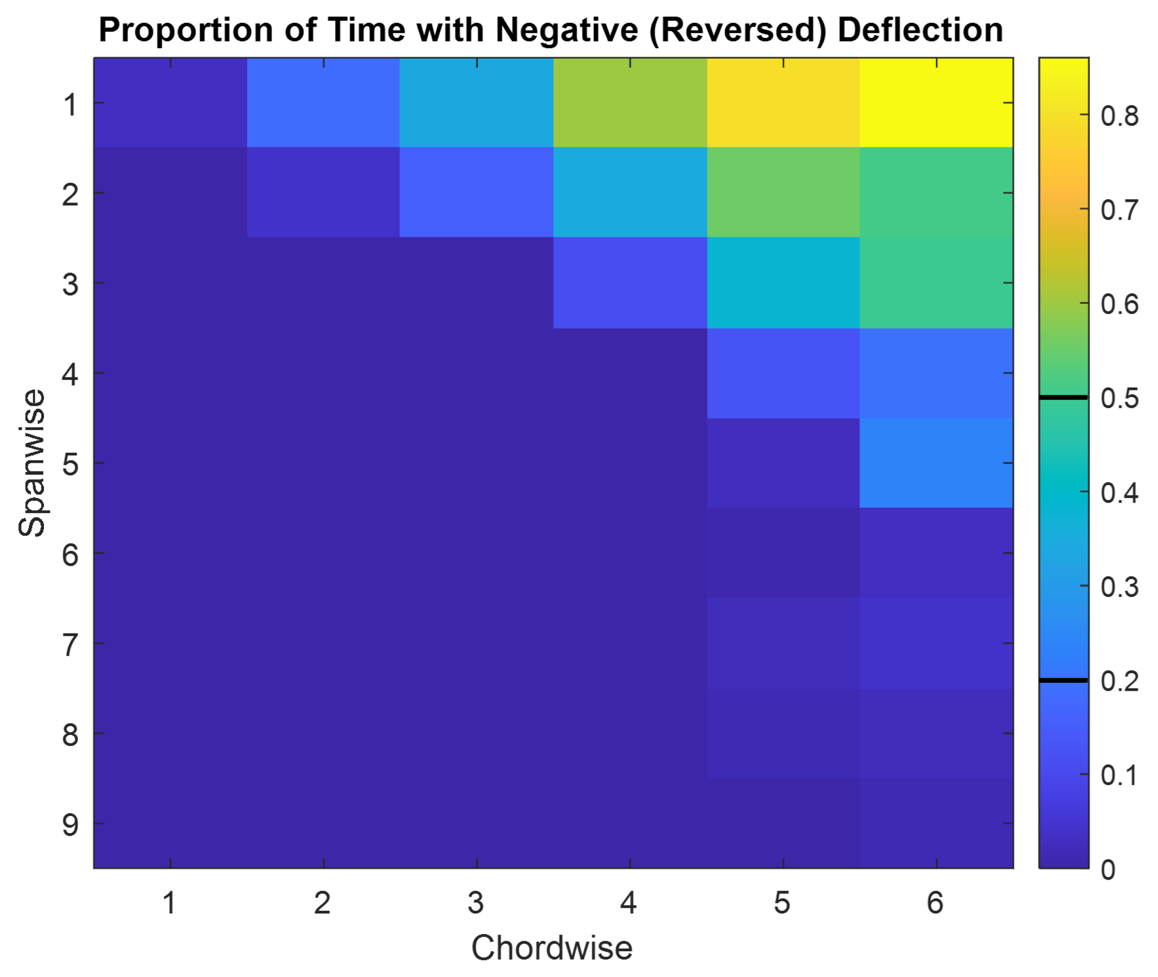
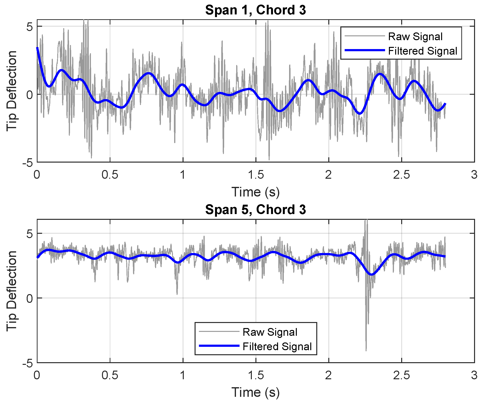
Figure 10,
Figure 11 and
Figure 12 are three indicators of reversed flow, and in a broader sense, incipient stall. The chord-wise profiles showed a characteristic change in the slope of the mean tip deflection distribution, indicating the rate of growth in the boundary layer and highlights that at the root section. The mean tip deflection heat-map further supported this by highlighting regions of diminished deflection magnitude toward the trailing edge, consistent with localized growth in boundary layer and reduction in bulk flow effect on pillar deflection. Finally, the reversal heat-map illustrated the frequency of negative deflections. This provides direct evidence of intermittent or persistent flow reversal at the inboard sections before progressing outward along the span, which was seen in [
14] as a marker of incipient stall. Together, these results validate the array’s ability to detect stall development spatially and temporally.
While the use of the NACA0012 aerofoil limits the geometric complexity of the present study, it provided a necessary and well-characterised baseline for validating sensor behaviour under controlled flow separation conditions. Future work will focus on extending the sensor array testing to more complex and application-specific aerofoil geometries, including those relevant to UAV and morphing-wing platforms.
5. Conclusions
This paper continues investigating the application of optically tracked flexible pillar sensors in flow detection and characterisation over the wing of an NACA0012 aerofoil section, and by extension draws insights into the feasibility of using such systems in a fly-by-feel, small-to-medium-scale UAV. The results of the experiments carried out demonstrated how distributed sensing enhances a UAV’s ability to detect airflow separation, turbulence, and stall onset. Experiments using a flexible optically tracked pillar sensor array mounted on a washed-out wing clearly indicated early stall onset on the inboard section through increased deflection fluctuations, frequent flow reversal events, and characteristic low-frequency oscillations.
Compared to conventional UAV control systems that rely on sparse point sensing on the airframe, this study reinforced the advantages of distributed aerodynamic sensing architectures observed in natural fliers. Unlike conventional approaches such as pitot probes, pressure taps, or hot-wire sensors, which provide information at a limited number of discrete locations, the distributed pillar array enables simultaneous observation of flow-state development across the aircraft surface. This facilitates the simultaneous detection of a variety of flow phenomena. The results align with previous work on detecting aerofoil flow phenomena, specifically, incipient stall, using a single row of optically tracked flexible pillar sensors, while also introducing new opportunities for real-time adaptive flight control informed by distributed flow-state sensing. The paper highlighted how sensor placement and response sensitivity have an impact on the information gleaned, which had not been fully explored in prior studies.
Table 2 provides a qualitative comparison between the present sensing architecture and conventional aerodynamic sensing technologies [
27,
28,
29].
The study employed optical tracking of fluorescent tips on flexible pillar sensors, removing the need for physical wiring to each sensing element. In practical UAV applications, this could be implemented using low-cost onboard optical systems focused on key regions of interest. While the present setup used high-speed cameras with optical wavelength filtering and offline post-processing, the approach establishes a foundation for using lightweight, commercially available imaging hardware with onboard data processing. Additionally, ongoing work involving event-based cameras calibrated for flow-specific features shows promise for significantly reducing system complexity and computational overhead. While this study uses optical tracking, the approach is compatible with other methods such as piezoelectric or fibre-optic transmission, enabling future onboard integration in UAV platforms. The experimental validation presented contributes to bridging the gap between biological mechanosensation and distributed aerodynamic sensing for UAV systems.
The experiments were carried out in a controlled environment where the effects of some real-world flight scenarios might not be apparent. Specifically, the water-based tests were conducted at Reynolds numbers on the lower end of what small to medium UAVs would typically encounter in air. The increased fluid density of water also influenced the dynamic response of the pillars through added mass and damping effects, resulting in a lower measured natural frequency than previously reported for the same sensor geometry in air. This effect as discussed in
Section 2 should be considered when extrapolating sensor dynamics to airborne applications. Additionally, the application of signal filtering, while effective at isolating low-frequency flow phenomena, inevitably attenuates higher-frequency content that may carry useful flow dynamics. Environmental factors such as reduced visibility, which could impair optical tracking, and conditions like icing, which could alter the mechanical response of the sensors, were also not represented in the present study.
Future work should therefore aim to run wind-tunnel experiments on more complex geometries with an integrated ’online’ processing in a more repeatable setup, in addition to implementing the sensors into a test-bed UAV and evaluating the system across a range of flight conditions and operational platforms, and to quantitatively assess the impact of the sensor array in comparison to currently deployed aerodynamic sensing hardware. Furthermore, the integration of advanced machine learning algorithms in the characterisation and interpretation of data from distributed sensor arrays [
30,
31,
32] offers a promising path toward more adaptable and robust deployment strategies. Recent work has similarly demonstrated the capability of distributed aerodynamic sensing architectures to estimate aerodynamic state information across a wide range of flight conditions, in line with the future development of fly-by-feel UAV systems [
33]. In summary, this paper demonstrates the viability of bio-inspired distributed flow sensing in UAVs, highlighting its potential to enhance stability, control, and energy efficiency.