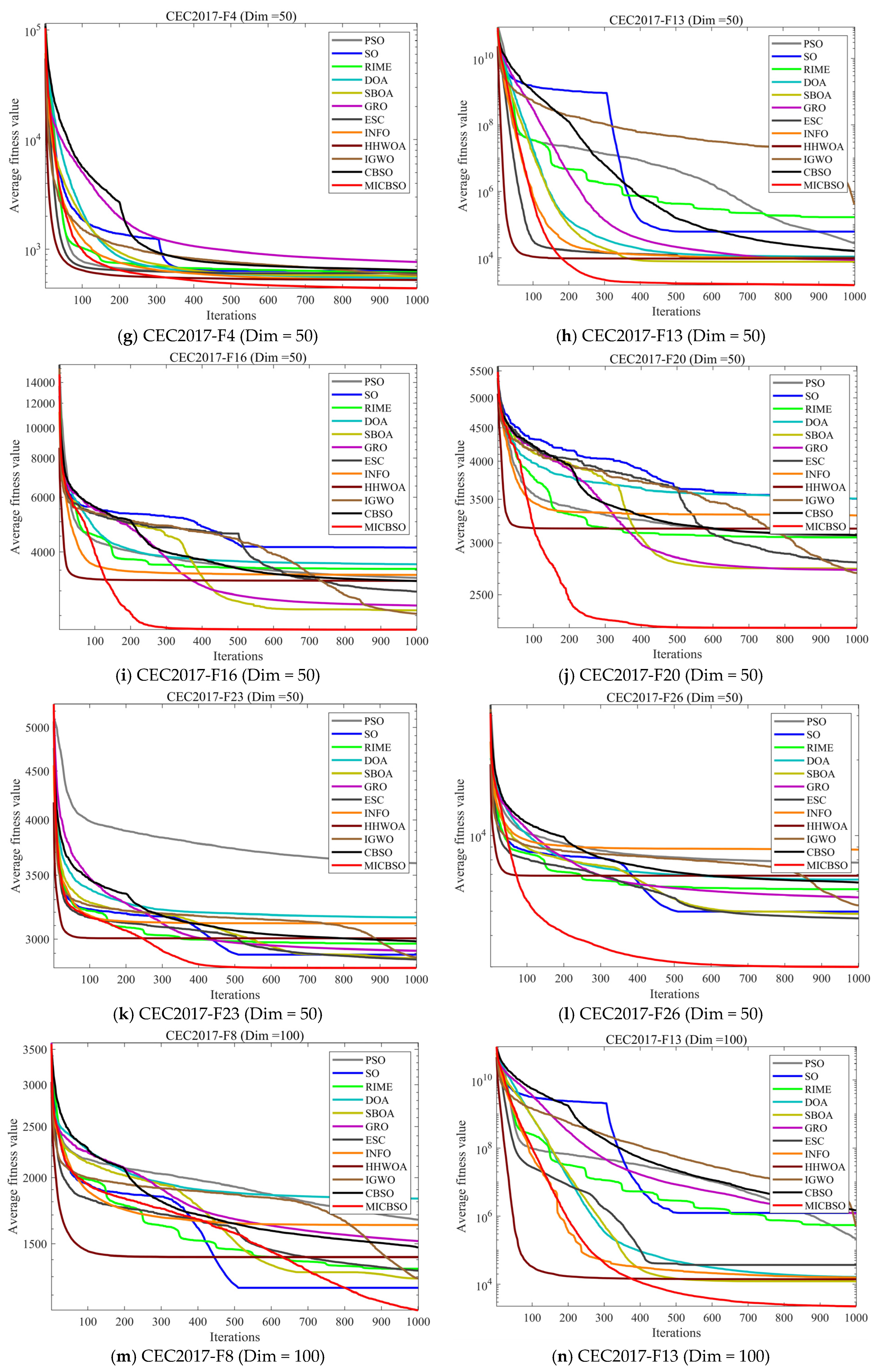
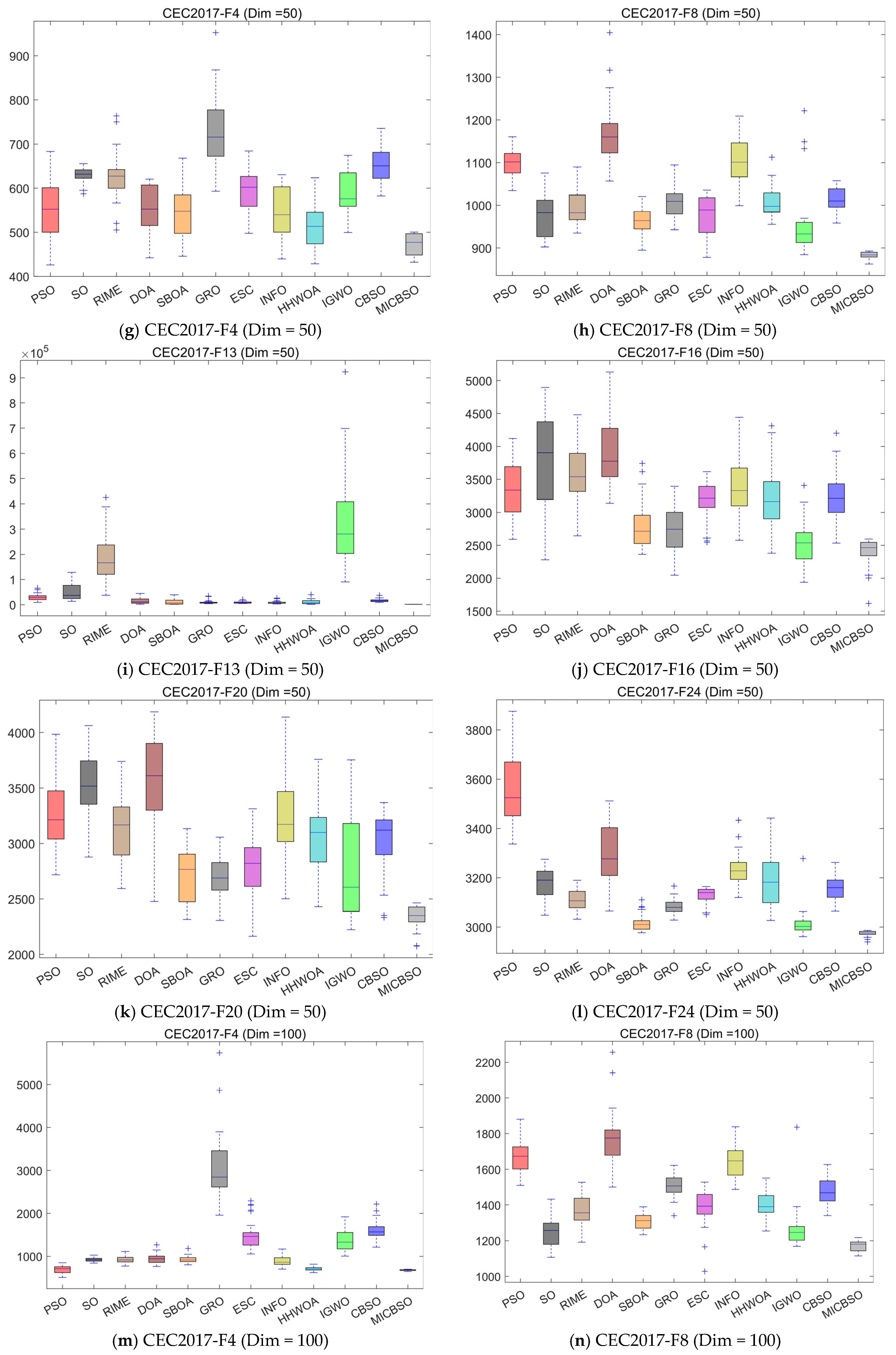
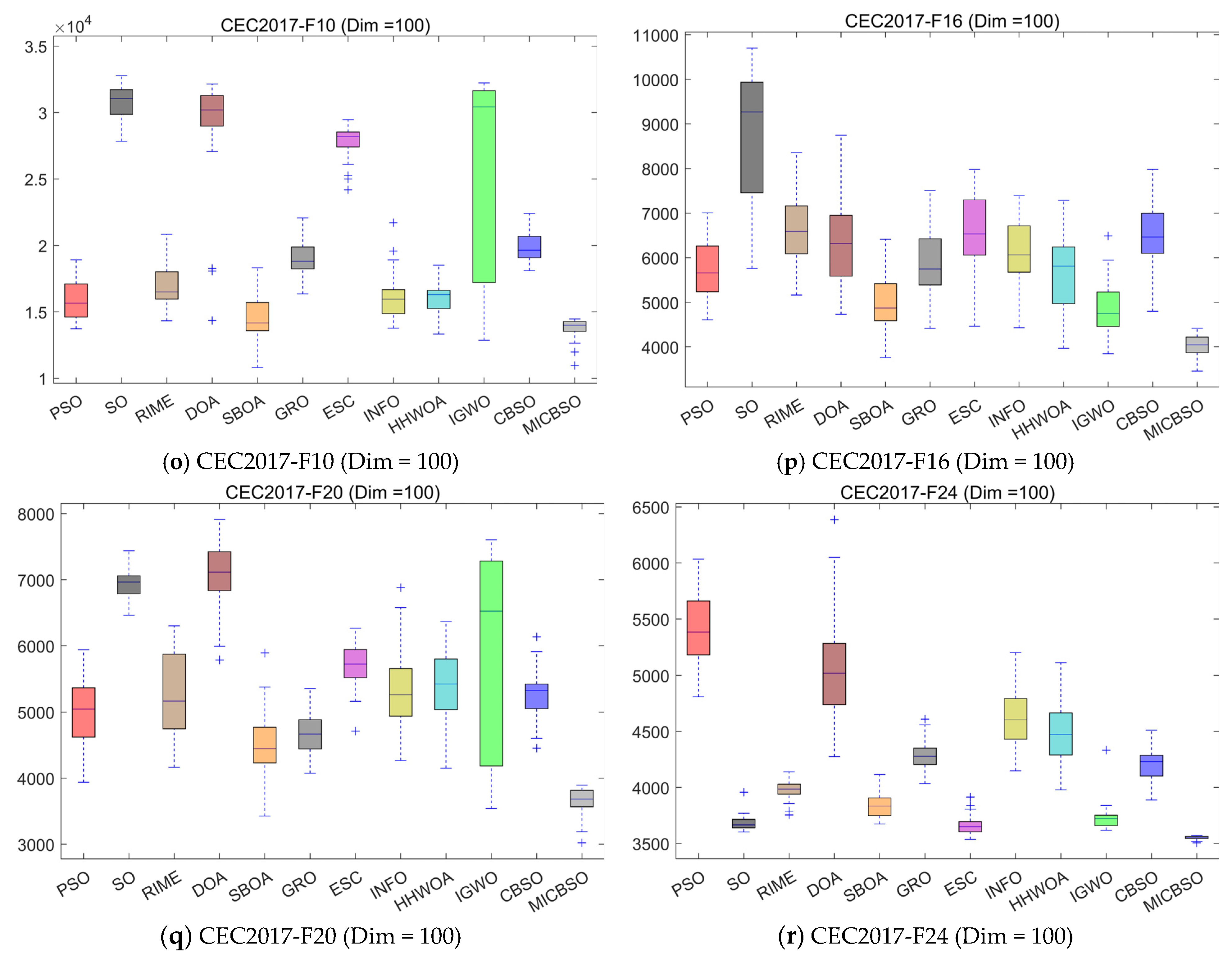
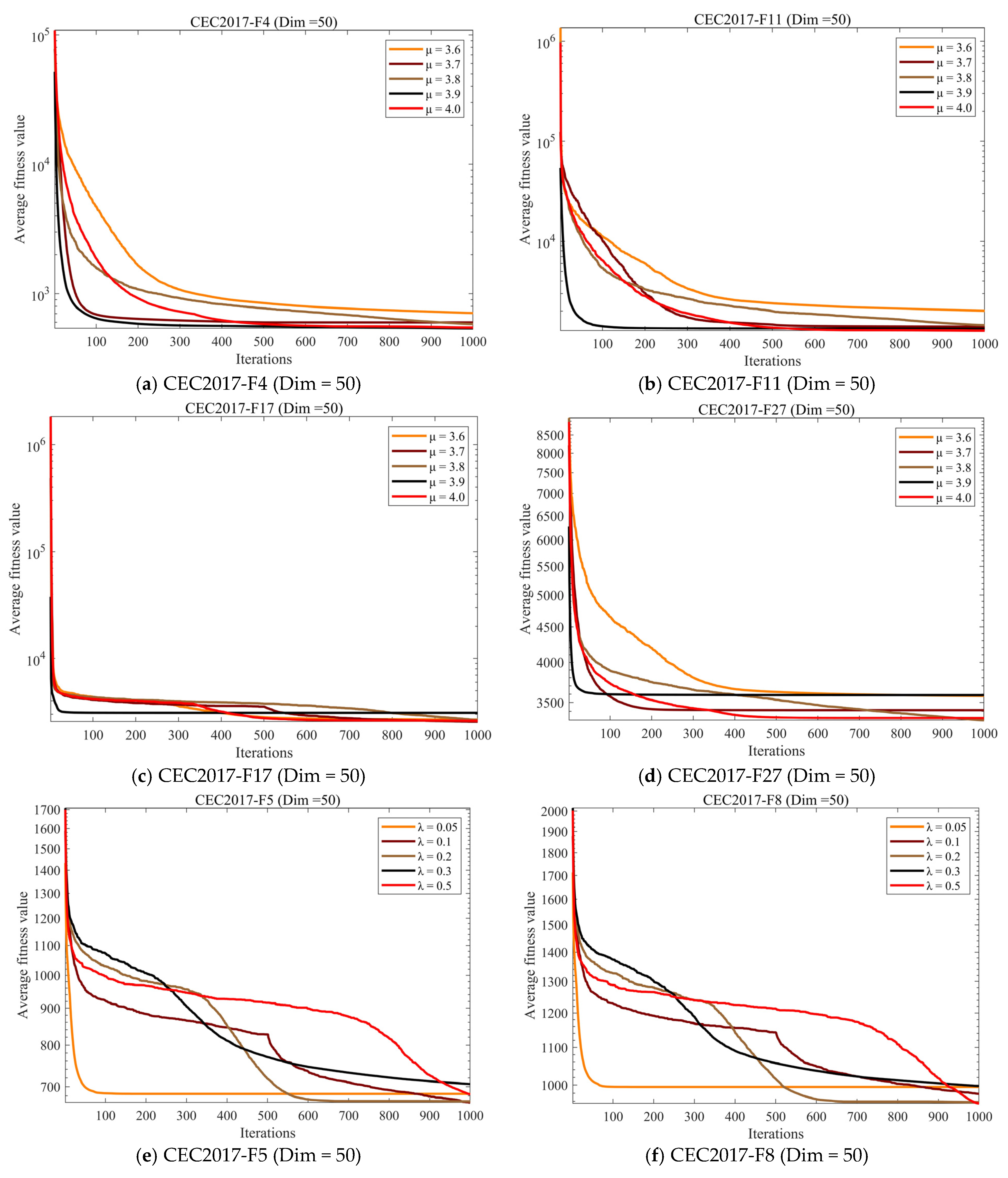
While CBSO performs well on 15-, 18-, and 25-rod problems, No Free Lunch theorems state that each algorithm requires modification for specific problems to improve its performance. Therefore, this paper proposes three effective strategies to enhance CBSO, described in detail below.
Throughout this paper, random variables are denoted in a unified manner. Unless otherwise specified, , , , and represent mutually independent scalar random variables uniformly distributed in . Similarly, denotes a random vector whose elements are independently sampled from . The vectors and denote Gaussian random vectors sampled from , and denotes a Lévy-distributed random vector. In addition, is used only as the initial seed of the Logistic chaotic map, and it is randomly sampled from . With this notation, repeated explanations such as “a random number between 0 and 1” are omitted in the following equations.
3.1. Population Initialization Strategy Based on Chaos-Opposition Learning
During the population initialization phase, the CBSO employs a random initialization method to obtain the initial population, which may result in inconsistent quality among initial populations [
15]. To further improve the distribution quality and global exploration capability of the initial population, MICBSO introduces a joint strategy of Chaotic Map and Opposition-based Learning (OBL) in the algorithm initialization stage, forming a more diverse and globally comprehensive initialization method. In this method, a chaotic sequence is first generated through a Logistic mapping [
16], which can be specifically represented by Equation (7).
where
is a control parameter with a value of 4. In this study, the Logistic map with
is adopted to generate the chaotic sequence for population initialization. The main reason is that, when
, the Logistic map exhibits strong chaotic behavior, simple mathematical implementation, and low computational cost, which makes it suitable for large-scale repeated optimization experiments. Compared with some other chaotic maps, such as Tent, Sine, Circle, and Chebyshev maps, the Logistic map does not require complicated parameter adjustment and can generate a sufficiently irregular sequence within the interval
. This property is consistent with the initialization requirement of MICBSO, where the chaotic sequence is directly mapped into the search space to improve population coverage.
is a random number between 0 and 1, and then through long-term iteration, a uniformly distributed sequence is obtained. The initial value
is an important factor affecting the trajectory of a chaotic sequence. In the proposed MICBSO,
is not treated as a manually tuned control parameter, but is randomly generated within the interval
for each independent run. This design avoids the dependence of the algorithm on a fixed chaotic seed and reduces the risk that the initial population is biased by a specific
. In addition,
is set to 4 so that the Logistic map enters a fully chaotic state, enabling the generated sequence to exhibit strong randomness and ergodicity. To avoid degenerate cases,
should not be set to boundary or special values such as 0, 0.25, 0.5, 0.75, or 1, which may lead to fixed points or short-period behavior. Since
is randomly sampled in each run and all algorithms are independently executed 30 times, the influence of different initial chaotic seeds is statistically averaged in the reported results. Therefore, the performance of MICBSO is not determined by a single fixed
, but by the overall population distribution generated through random chaotic initialization and opposition-based learning. Then, by linearly mapping
to the search space of the current dimension, we can obtain the initial search agent, which can be expressed by Equation (8). To clarify the rationale for selecting the Logistic map,
Table 1 compares several commonly used chaotic maps across dimensions such as mathematical form, parameter settings, implementation complexity, and applicability to the proposed MICBSO initialization framework.
Compared with traditional random initialization, chaotic mapping has better ergodicity and uniformity of distribution, which can avoid the initial solutions from being concentrated in local regions of the search space, thus providing a higher quality starting point for subsequent global searches.
After obtaining the chaotic initial population, this paper further introduces an opposition learning mechanism to construct its opposition solution for each individual in order to expand the search range. For the
-th individual, its opposite individual
is calculated using Equation (9).
It can be seen that
and
are symmetrical about the center of the interval
. Thus, while generating a candidate solution, a “mirror solution” on the other side of the search space is also generated, which is equivalent to sampling the search space from two directions at the same time. Subsequently, fitness was calculated for the original individual and its counterpart using Equation (10).
In this study, a one-to-one competition selection mechanism is adopted after evaluating the original and opposite solutions. Specifically, each original individual
only competes with its corresponding opposite individual
, rather than selecting the best
individuals from the combined
candidates. For a minimization problem, the final initialized individual is determined as follows:
Through this one-to-one selection rule, the population size remains , and each original–opposite pair contributes one candidate solution to the final initial population. Compared with selecting the best individuals from all candidates, the one-to-one competition avoids excessive concentration of the initial population around several high-quality regions, thereby preserving the complementary sampling property of opposition-based learning. Meanwhile, this selection process does not introduce additional sorting operations and only requires fitness evaluations during initialization.
Following the principle of “survival of the fittest,” individuals with better fitness were selected as the final initialization individuals. In summary, the proposed chaotic-opposition joint initialization strategy generates initial candidate solutions through a Logistic chaotic mapping, ensuring good ergodicity and uniform distribution of solutions in the search space. For each candidate solution, an opposite solution is constructed and selectively retained. Sampling is performed from two directions in the search space to expand the search range. The resulting initial population exhibits both high diversity and high average fitness. Compared to traditional random initialization methods, the chaotic-opposition joint strategy significantly improves the algorithm’s global search capability, reduces the probability of the algorithm getting trapped in local optima, and accelerates early convergence.
As shown in
Table 1, although Tent, Sine, Circle, and Chebyshev maps also have chaotic properties and can be used for population initialization, they may introduce piecewise computation, additional control parameters, stronger oscillation, or extra normalization procedures. In contrast, the Logistic map with μ = 4 has a compact mathematical expression, requires no additional parameter adjustment, and can generate chaotic sequences directly within the interval (0, 1). This makes it suitable for the proposed chaos–opposition learning initialization strategy, where the chaotic individuals and their opposite solutions are jointly evaluated to improve initial search coverage. Therefore, the Logistic map is selected as the chaotic sequence generator in MICBSO.
3.2. Multi-Elite Guidance Mechanism Based on Gaussian Perturbation
To enhance the exploitation capability of CBSO while maintaining sufficient global search ability, a Gaussian perturbation-based multi-elite guidance mechanism is proposed in MICBSO. In the original CBSO, the population update process is strongly influenced by the current best solution. Although this mechanism can accelerate convergence, it may also cause excessive dependence on a single elite individual. Once the current best solution is located near a local optimum, the search direction of the whole population may be misled, resulting in premature convergence and insufficient population diversity.
To alleviate this problem, MICBSO introduces a multi-elite guidance mechanism. Instead of using only the current global best solution as the guiding point, the proposed mechanism uses the average information of the top
elite individuals to construct a more stable guidance vector. Meanwhile, Gaussian perturbation is introduced to provide stochastic search ability around the elite region, which helps the population escape local optima and improves the balance between exploration and exploitation. The position update formula of the proposed multi-elite guidance mechanism is expressed as follows:
where
denotes the position of the
-th individual at iteration
,
is the multi-elite guidance vector, and
represents the Gaussian perturbation direction of the
-th individual. The adaptive coefficients
and
are used to control the influence of multi-elite guidance and Gaussian perturbation, respectively.
The coefficient
controls the attraction strength toward the multi-elite guidance center. It is defined as a linearly decreasing function:
where
is the initial guidance coefficient,
is the current iteration number, and
is the maximum number of iterations. In the early stage, a larger
helps individuals move toward promising regions identified by multiple elites. As the iteration proceeds,
gradually decreases, which prevents excessive attraction to the elite center and reduces the risk of population aggregation in the later stage.
The coefficient
controls the influence of the Gaussian perturbation term. It is defined as an exponentially decreasing function:
where
is the initial perturbation coefficient and
is the exponential decay factor. The exponential decay form enables the Gaussian perturbation to play a stronger role in the early search stage and decrease rapidly in the middle and later stages. Therefore, the algorithm can maintain stronger exploration ability at the beginning and reduce unnecessary random disturbance during local refinement.
In Equation (12),
denotes the perturbation direction generated by the Gaussian-mutated elite solution. To clarify its relationship with the Gaussian-mutated solution,
is first constructed around the current best solution:
where
denotes the current best solution, and
represents a standard Gaussian random vector with zero mean and unit variance. Then, the perturbation direction of the
-th individual is defined as the difference between the Gaussian-mutated elite solution and the current individual:
Thus, Equation (12) can be further understood as a combination of two search directions: the first one is the attraction direction from the current individual to the multi-elite guidance center , and the second one is the stochastic perturbation direction from the current individual to the Gaussian-mutated elite solution . This formulation enables MICBSO to exploit high-quality elite information while maintaining a certain degree of randomness.
The multi-elite guidance vector
is calculated by averaging the positions of the top
elite individuals:
where
denotes the
-th elite individual after ranking the population according to fitness values. In this study,
is adopted. Compared with single-best guidance, the use of multiple elite individuals can reduce the risk of search bias caused by one potentially misleading best solution. However, if
is too small, the algorithm may still suffer from excessive dependence on a few individuals; if
is too large, medium-quality individuals may weaken the guidance effect of high-quality solutions. Therefore, a parameter sensitivity analysis for
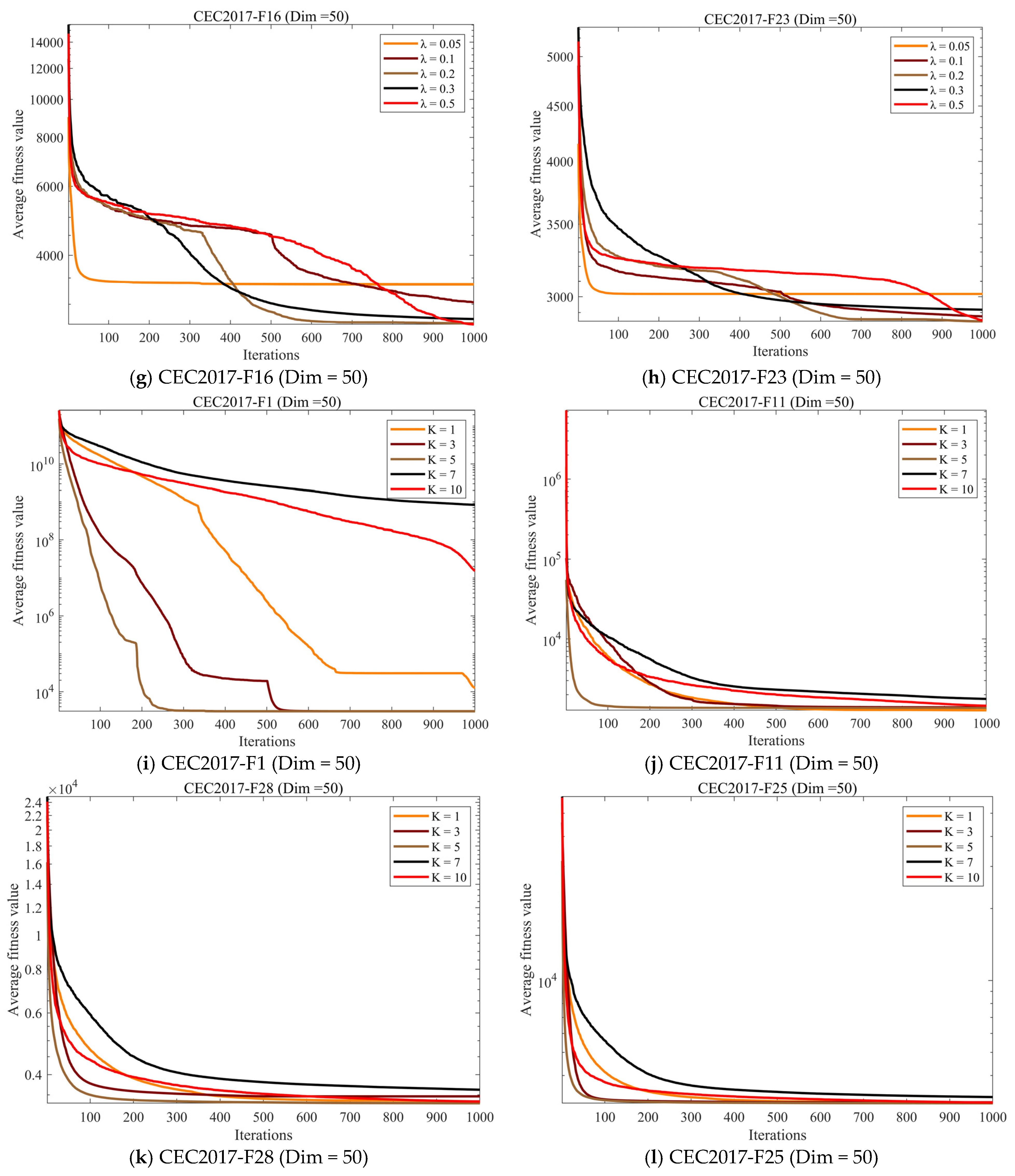
is conducted in
Section 4.8 to justify this setting.
Although
in Equation (15) is a standard Gaussian random vector with fixed unit variance, the actual perturbation intensity in MICBSO is not fixed. This is because the Gaussian random vector is scaled by
in Equation (15), and its influence on the final position update is further controlled by
in Equation (12). According to Equations (12), (15) and (16), the stochastic component introduced into the position update is mainly determined by
Therefore, the effective variance of the stochastic Gaussian perturbation can be expressed as
Since decreases linearly and decreases exponentially with the iteration process, the effective perturbation variance also gradually decreases. In the early stage, a relatively large effective variance helps the population explore a wider search region and avoid premature convergence. In the later stage, the reduced effective variance weakens random disturbance and allows the algorithm to focus on local exploitation around promising regions. Therefore, although the standard Gaussian distribution itself has a fixed unit variance, the effective perturbation strength in MICBSO is adaptively controlled by and .
The parameters , , and are used to determine the decreasing trend of the multi-elite guidance strength and Gaussian perturbation intensity. In this study, , , and are adopted. Specifically, provides a relatively strong but not excessive attraction toward the multi-elite guidance center in the early search stage. Since gradually decreases to 0 as the iteration proceeds, it helps avoid excessive elite attraction in the later stage. The value keeps the initial Gaussian perturbation at a normal scale, while makes the perturbation term decrease rapidly in the middle and later stages. For example, when , , and when , . Therefore, Gaussian perturbation plays a stronger role in early exploration and becomes very weak during late exploitation.
The reason for adopting linear decay for and exponential decay for is that these two coefficients control different search behaviors. The multi-elite guidance term should decrease smoothly to avoid abrupt changes in the search direction; therefore, a linear decay function is used for . In contrast, Gaussian perturbation should be strong in the early stage but rapidly weakened in the later stage to improve convergence stability; therefore, an exponential decay function is used for . Compared with other adaptiv schedules, such as polynomial decay, cosine decay, sigmoid decay, or feedback-based adaptive adjustment, the adopted linear–exponential combination has a simpler structure and introduces fewer additional parameters. This helps MICBSO achieve a smooth transition from global exploration to local exploitation while maintaining low parameter complexity.
To further clarify the selection of the adaptive schedules,
Table 2 provides a qualitative comparison of several commonly used decay functions.
As shown in
Table 2, alternative adaptive schedules may provide more flexible adjustment, but they usually introduce additional parameters or require extra monitoring of the search process. In contrast, the proposed linear–exponential decay design provides a simple and effective two-level control mechanism. The linear decay of
ensures that the multi-elite guidance strength decreases smoothly, while the exponential decay of
rapidly reduces the influence of Gaussian perturbation in the later stage. Therefore, this mechanism can maintain sufficient exploration in the early stage and enhance convergence stability in the later stage without significantly increasing parameter complexity.
3.3. Hybrid Boundary Control Strategy Based on Random Reflection
In CBSO, it is common for individuals to go out of bounds during the search process. Out-of-bounds individuals not only lead to infeasible solutions but may also cause the loss of search direction information, resulting in premature convergence and insufficient utilization of the solution space. In particular, the CBSO algorithm has a strong tendency for jump-up updates; therefore, designing a robust and efficient boundary handling mechanism is crucial for improving algorithm performance. To this end, this paper adopts a hybrid boundary strategy that combines reflective boundary control with a random reset mechanism, which takes into account the feasibility of understanding, the consistency of search direction, and the maintenance of population diversity [
22].
For boundary crossing situations, MICBSO first adopts a boundary reflection strategy. When an individual exceeds the search interval in a certain dimension, the boundary is used as the axis of symmetry to reflect the position back to the feasible region, which can be expressed as Equation (20).
Furthermore, while reflective boundaries can handle most out-of-bounds situations, for individuals with large overshoots or repeated violations, reflection alone may cause the individual to oscillate near the feasible region boundary. To avoid this problem, MICBSO introduces a random reinitialization strategy, which resamples the dimensions of large overshoots into the search space, as expressed in Equation (21).
where
is a random number between 0 and 1. Combining the two strategies mentioned above, MICBSO’s boundary control mechanism can be expressed as Equation (22).
where
is the reflection threshold, used to distinguish between minor and severe boundary violations. Specifically, it can be expressed by Equation (23). Where
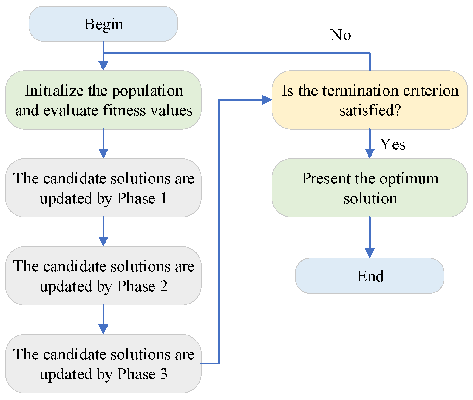
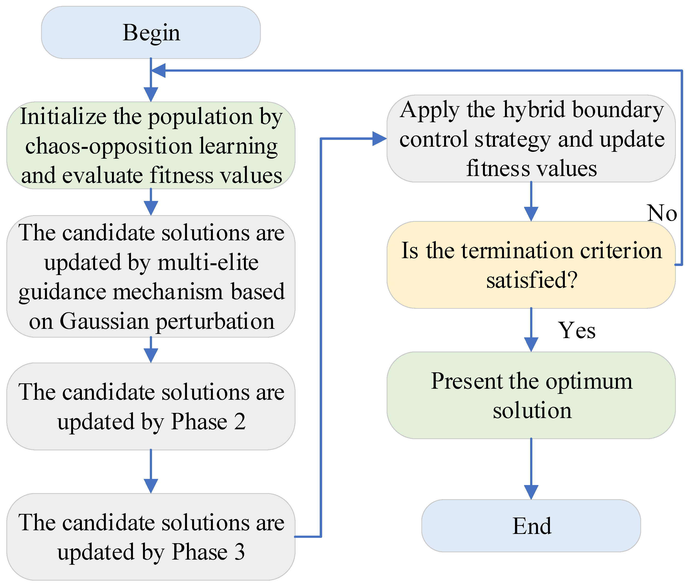
Figure 2 shows the flowchart of MICBSO. It should be noted that MICBSO does not apply multiple reflections for repeatedly out-of-bounds individuals. The reason is that repeated reflection may cause individuals with large violations to oscillate near the boundary or even remain infeasible under large overshoot conditions. Therefore, the proposed hybrid boundary control strategy only applies a single reflection to minor boundary violations. Specifically, when
or
, the individual is reflected once back to the feasible region. Since
is smaller than the search range, the reflected position will still fall within the feasible interval. For example, if
and
, then the reflected value satisfies
, which is feasible. For severe boundary violations, reflection is not used. Instead, the violated dimension is randomly reinitialized within the feasible interval according to Equation (21). This design avoids repeated boundary oscillation and ensures that the corrected position always satisfies the boundary constraint. In addition, after boundary handling, a final feasibility check is conducted to guarantee that all decision variables remain within
.
The threshold coefficient 0.2 is adopted to provide a moderate boundary-handling range. If the threshold is too small, most out-of-bounds individuals will be regarded as severe violations and randomly reinitialized, which may weaken the continuity of the search direction. If the threshold is too large, most boundary violations will be handled by reflection, which may cause individuals to oscillate near the boundary and reduce population diversity. Therefore,
is used as a balanced setting between reflective correction and random reinitialization. To further justify this setting, a parameter sensitivity analysis of
in
is conducted in
Section 4.8. The results show that
achieves more stable convergence performance than too small or too large threshold settings.
Although chaotic initialization, opposition-based learning, Gaussian perturbation, and boundary control have been employed in some existing improved swarm intelligence algorithms, the proposed MICBSO differs from these methods in its algorithm-specific integration with the three-stage search mechanism of CBSO. Existing studies usually introduce these strategies as independent enhancement operators to improve either initialization quality, local perturbation, or boundary repair separately. In contrast, MICBSO constructs a coordinated optimization framework in which the chaos–opposition learning strategy first improves the distribution quality and search coverage of the initial banking entities; the Gaussian perturbation-based multi-elite guidance mechanism then replaces the single-best-oriented guidance tendency of CBSO with a more stable elite-group-driven search direction; and the hybrid boundary control strategy adaptively combines reflection and random reinitialization to preserve feasible search directions while avoiding repeated boundary stagnation. Therefore, the novelty of MICBSO does not lie in using these operators in isolation, but in coupling them with the banking-system-inspired search process of CBSO to form a stage-aware balance among initialization diversity, elite-guided exploitation, and feasibility preservation. This coordinated design is particularly suitable for high-dimensional numerical optimization and constrained three-dimensional UAV path planning, where premature convergence, infeasible solutions, and unstable search trajectories frequently occur.
To further clarify the difference between the proposed hybrid boundary control strategy and common boundary-handling methods, several representative techniques are compared in
Table 3, including saturation, periodic mapping, random repair, pure reflection, and the proposed hybrid strategy.
Compared with saturation and periodic mapping, the proposed hybrid boundary control strategy can avoid excessive concentration near the boundary and does not assume periodic characteristics of the search space. Compared with pure random repair, MICBSO preserves useful search direction information for minor boundary violations through reflective correction. Compared with pure reflection, MICBSO avoids repeated boundary oscillation by applying random reinitialization to severe violations. Therefore, the proposed hybrid strategy provides a more flexible boundary-handling mechanism by balancing feasibility preservation, search continuity, and population diversity.
3.4. Time Complexity Analysis and Execution Time Comparison
To further analyze the computational cost introduced by the proposed improvement strategies, the time complexity of MICBSO is discussed in this subsection. Assume that the population size is , the problem dimension is , the maximum number of iterations is , the number of selected elite individuals is , and the computational cost of one fitness evaluation is .
For the original CBSO, the population initialization requires
operations, and the corresponding fitness evaluation requires
. During each iteration, the position update of all candidate solutions requires approximately
, and the fitness evaluation requires
. Therefore, the overall time complexity of CBSO can be approximately expressed as:
For the proposed MICBSO, the chaos–opposition learning initialization strategy introduces additional computational cost in the initialization stage. Specifically, the Logistic chaotic map is first used to generate
chaotic candidate solutions, which requires
. Then, opposition-based learning generates another
opposite candidate solutions, which also requires
. Since both the chaotic individuals and their opposite solutions need to be evaluated, the number of fitness evaluations in the initialization stage increases from
to
. Therefore, the initialization complexity of MICBSO can be expressed as:
Although the opposition-based learning mechanism doubles the number of fitness evaluations during initialization, this additional cost is only introduced once before the iterative search begins. In contrast, the main computational cost of metaheuristic algorithms usually comes from repeated fitness evaluations during the iterative optimization process. If each individual is evaluated once per iteration, the total number of fitness evaluations in the original CBSO is approximately
where
evaluations are used for initialization and
evaluations are used during iterations. For MICBSO, due to the additional opposite solutions in the initialization stage, the total number of fitness evaluations becomes
Thus, the relative increase in fitness evaluations caused by the chaos–opposition learning initialization strategy is
In this study, the maximum number of iterations is set to . Therefore, the additional fitness evaluation cost introduced by opposition-based learning is approximately , namely about of the total fitness evaluations. This indicates that although the initialization stage requires more evaluations, the additional computational burden is very limited in the whole optimization process.
In the iterative stage, the Gaussian perturbation-based multi-elite guidance mechanism introduces several additional operations. First, the population needs to be ranked or selected to obtain the top
elite individuals. This process requires
if sorting is used. Then, the elite guidance vector
is constructed using the selected
elite individuals, requiring
. The Gaussian perturbation and position update operations require
. Since
is much smaller than
in this study, and
is adopted, the additional cost of constructing the elite guidance vector is relatively small. Therefore, the time complexity of the multi-elite guidance mechanism can be approximately expressed as:
The hybrid boundary control strategy checks and repairs each dimension of each candidate solution. Therefore, its computational complexity is Combining the above analyses, the total time complexity of MICBSO can be expressed as
Since and the fitness evaluation cost is usually the dominant part in benchmark optimization and UAV path planning problems, the additional computational cost introduced by the proposed strategies does not change the overall order of complexity. Therefore, the asymptotic time complexity of MICBSO can be simplified as Compared with the original CBSO, MICBSO introduces extra computational operations mainly from three aspects: opposite solution evaluation during initialization, elite selection and guidance vector construction, and hybrid boundary repair. However, the opposition-based learning strategy only increases the initialization evaluations once, the number of elite individuals is small, and the boundary control strategy only involves simple dimension-wise judgment and correction. Therefore, the additional computational burden of MICBSO is acceptable. More importantly, these strategies improve the initial population quality, reduce the risk of premature convergence, and enhance solution feasibility, which can help the algorithm obtain better solutions within the same maximum iteration number.
The theoretical comparison between CBSO and MICBSO is summarized in
Table 4.
From
Table 4, it can be observed that MICBSO has a slightly higher computational cost than CBSO due to the introduced improvement strategies. However, the increased cost is mainly reflected in the initialization stage and simple auxiliary update operations. The chaos–opposition learning strategy doubles the number of fitness evaluations only during initialization, while the total additional evaluation ratio is only
. Therefore, under the experimental setting of
, the additional computational burden is very small compared with the entire optimization process. This demonstrates that MICBSO improves optimization performance while maintaining acceptable computational complexity.
In addition, we tested the various algorithms on the CEC2017 test set and recorded their actual execution times; the experimental results are shown below.
As shown in
Table 5, the execution time of all algorithms increases as the problem dimension grows from 30 to 100, indicating that higher-dimensional optimization problems require more computational resources. Compared with the original CBSO, MICBSO introduces additional operations, including chaos–opposition-based initialization, multi-elite guidance, Gaussian perturbation, and hybrid boundary control. Therefore, its runtime is slightly higher than that of CBSO. Specifically, the runtime of MICBSO is 23.94 s, 48.33 s, and 172.33 s for Dim = 30, Dim = 50, and Dim = 100, respectively, while the corresponding runtime of CBSO is 22.60 s, 43.49 s, and 150.38 s. The relative increases are approximately 5.93%, 11.13%, and 14.60%, respectively. This indicates that the additional computational cost introduced by the proposed improvement strategies is limited. The proof of the global convergence of MICBSO is presented in
Appendix A.
Although MICBSO is not the fastest algorithm, its runtime remains within an acceptable range. For example, under Dim = 30 and Dim = 50, MICBSO is faster than several comparison algorithms, such as ESC, HHWOA, and IGWO. Under Dim = 100, MICBSO is still much faster than HHWOA and IGWO, and its runtime is close to ESC. More importantly, the slightly increased runtime mainly comes from auxiliary operations rather than repeated expensive fitness evaluations. The chaos–opposition-based initialization only increases the number of fitness evaluations once at the beginning, while the multi-elite guidance and boundary control strategies mainly involve simple vector operations and boundary checks. Therefore, the proposed strategies do not cause excessive computational burden.
Overall, the execution time results demonstrate that MICBSO achieves a reasonable trade-off between computational cost and optimization performance. Although it requires slightly more time than CBSO, the additional runtime is acceptable considering its improved convergence accuracy, robustness, and solution quality. Therefore, MICBSO maintains practical computational efficiency while enhancing the overall optimization capability.